2 Size and Shape, Scale and Dimension

Size

and

Shape, Scale

and

Dimension

We are here face to face with the crucial paradox of knowledge. Year by year we devise more precise instruments with which to observe nature with more fineness. And when we look at the observations, we are discomforted to see that they are all still fuzzy and we feel that they are as uncertain as ever. We seem to be running after a goal which lurches away from us to infinity every time we come within sight of it. (Bronowski, 1973, p. 256.)

2.1

Scale, Hierarchy and Self-Similarity

We have already seen in Chapter 1 that cities are organized hierarchically into distinct neighborhoods, their spatial extent depending upon the econ-omic functions which they offer to their surrounding population. This hier-archy of functions exists throughout the city, with the more specialized serving larger areas of the city than those which meet more immediate and local needs. The centers and their hinterlands which form this hierarchy have many elements in common in functional terms which are repeated across several spatial scales, and in this sense, districts of different sizes at different levels in the hierarchy have a similar structure. Moreover, the hierarchy of functions exists for economic necessity, and the growth of cities not only occurs through the addition of units of development at the most basic scale, but through increasing specialization of key centers, thus raising their importance in the hierarchy. These mechanisms of urban growth also ensure that the city is stable, in the sense portrayed in the previous chapter where hierarchical differentiation was associated with the process of building resilient systems (Simon, 1969).

Size and Shape, Scale and Dimension 59

transactions take place. Such structures which repeat themselves at different levels of the hierarchy and which in turn are associated with different scales and sizes are said to be self-similar. Moreover, it is this property of self-similarity that is writ large in the shape and form of cities, and provides the rationale for a new geometry of cities which is to be elaborated in this book. To make progress in tracing the link between urban form and function, we must now embark upon a more structured analysis of city systems. In this chapter, we will outline the rudiments of this new geometry of form and function which has been developed over the last two decades, and which we anticipated in our introduction and in the previous chapter. This geometry has been christened by its greatest advocate, Benoit Mandelbrot (1983), as a 'geometry of nature', and although its most graphic examples exist in nature, it is increasingly being used to explore the ways in which artificial or man-made systems develop and are organized. In this book, we will speculate on how this geometry can be applied to cities, and in this chapter we will present its rudiments, concentrating on natural forms, but gradually introducing and demonstrating man-made forms which have s~milarproperties.

When we talk of geometry, we usually talk of a geometry based on the straight line, the geometry of Euclid upon which our concept of dimension is based. Although most natural shapes that we can imagine are clearly not composed of straight lines, we are able to approximate any object to the desired degree by representing it as straight line segments. However, we can only make formal sense of such objects if we can represent the entire form of the object in ways in which we might apply the calculus of Newton and Leibnitz, and invariably with real objects this is notpos~ible.Itis some-times possible to make progress by studying gross simplifications of natural objects in which form is continuous and differentiable, but we are so accus-tomed to assuming that our understanding of natural objects must be based on atomistic principles that we often assume away any pattern and order which does not fit our Euclidean-Newtonian methods of analysis. In short, our understanding of natural form and how it relates to function has been woefully limited, usually lying beyond analysis.

neighbor-hoods meet these criteria and form the set of fractal objects which we will explore in this book.

The best way to begin describing fractals is by example. A coastline and a mountain are examples of natural fractals, a crumpled piece of paper an example of an artificial one. However, such irregularity which characterizes these objects is not entirely without order and this order is to be found in' fractals in terms of the following three principles. First, fractals are always self-similar, at least in some general sense. On whatever scale, and within a given range you examine a fractal, it will always appear to have the same shape or same degree of irregularity. The 'whole' will always be manifest in the 'parts'; look at a piece of rock broken off a mountain and you can see'the mountain in the part. Look at the twigs on the branches of a tree and you can see the whole tree in these, albeit at a much reduced scale.

Second, fractals can always be described in terms of ahierarchy of self-similar components. Fractals are ordered hierarchically across many scales and the tree is the classic example. In fact, the tree is a literal interpretation of the term hierarchy and as such, it represents the most fundamental of fractals. There are many other examples of hierarchy: as we indicated in the last chapter, the organization and spacing of cities as central places is such an order while the configuration of districts and neighborhoods, and spatial distribution of roads and other communications are hierarchically structured. The third principle relates to the irregularity of form. Here by irregularity we mean forms which are continuous but nowhere smooth, hence non-differentiable in terms of the calculus. This point is so important that we must elaborate upon it further.

Ifyou try to describe a coastline, you will encounter the following prob-lem. Ifyou measure its length from a map, the map will have been con-structed at a scale which omits lower level detail. Ifyou actually measure the length by walking along the beach, you will face a problem of knowing what scale or yardstick to use and deciding whether to measure around every rock and pebble. In essence, what you will get will be a length which is dependent on the scale you use, and as you use finer and finer scales down to microscopic levels even, the length of the coastline will continue to increase. We are forced to conclude that the coastline's length is 'infi-nitely'long or rather, that its absolute length has no meaning and the length given is always relative to the scale of measurement.

Size and Shape, Scale and Dimension 61

by fractional dimension. Mountains would thus have fractal dimensions between 2 and 3, as if they were sculpted out of a solid block, more than the plane but less than the volume (cube). Fractals, however, would not be restricted to simply the dimensions we can visualize between the point and the volume but could exist between any adjacent pairs of higher dimen-sions. Indeed, as Mandelbrot (1967) argued, such objects are more likely to be the rule than the exception with Euclidean being a special case of fractal geometry. Most objects would thus have fractional, not integral dimension. In this chapter, we will illustrate this geometry using idealized forms. In other words, we will present fractal geometry in terms of objects which are well-specified and manifest similarity across scales which we can model exactly. This is in contrast to most of the fractals illustrated in the rest of this book which will not be exact in terms of their self-similarity, but manifest similarities across scales which are ordered only in terms of their statistical distribution. In the sequel, we will begin by exploring the simplest of deter-ministic fractals - the Koch curve - and then we will use this to derive the basic mathematics used to describe fractal forms, in particular, emphasizing the meaning of fractal dimension. We will explore one-dimensional curves which fill two-dimensional space, hierarchies and tree structures, and we will then outline a rather different approach to fractals based upon repeated transformations used to generate their form at every scale. This approach which is largely due to Barnsley (1988a) is called Iterated Function Systems (IFS) and it provides a powerful way of illustrating the critical properties of fractals.

In this book, we will be speculating on the measurement of urban form in two ways: first in terms of boundaries around and within cities, and second, in terms of the way cities grow and fill the space available to them. Our ideas will be largely restricted to those fractals which exist between the one dimension of the line and the two dimensions of the plane. Our mathematics will be elementary, requiring no more than high school algebra and calculus, and when we introduce some trickier development we will explicitly present our algebra through all the needed steps. Another feature of our approach and indeed of the development of fractals generally is that it is easiest to work with them using computer graphics. Indeed some say that without computer graphics, fractals would certainly not have come alive in the last 20 years. We will thus present many computer graph-ics to illustrate these ideas, some of which will be in gray tones or black and white, and others in color (see color plate section).

2.2 The Geometry of the Koch Curve

at this new scale resultsina further elaboration of the object's geometry at yet a finer scale, and the process is thus continued indefinitely towards the limit. In practice, the iteration or recursion is stopped at a level below which further scaled copies of the original object are no longer visible in terms of the scale at which the fractal is being viewed. In essence, however, the true fractal only exists in the limit, and thus what we see is simply an approximation to it.

We illustrate this process in Figure 2.1 for the non-rectifiable curve intro-duced by Helge von Koch in 1904, where we show the initiator - a straight line, and the generator which replaces the line by four copies of itself arranged as a continuous line but scaled so that each copy is one third the length of the initiator. The recursion which defines the process is shown as a hierarchy, or cascade as we will term it, in Figure 2.1. The tree which defines this cascade is indicative of the generative process which at each level replaces each part of the object by four smaller parts. As we have already implied, the tree which defines the cascade is itself a fractal, and in the rest of this chapter we will define all our fractals in terms of initiators, generators and the cascade which forms the process of application. In some fractals, we will see their geometry in terms of the cascading tree much more clearly than in others.

The Koch curve is an excellent example of a line which is scaled up in length at each iteration through replacing each straight line acting as its initiator by a line four thirds the length of the initiator, ordered in fOUf continuous straight line segments. An even better illustration of this process for our purposes is given by the Koch island whose construction and the first three levels of its cascade is illustrated in Figure 2.2. In this case, the initiator is an equilateral triangle - the island, and the generator consists of scaling the triangle to one which is one third the length of each of the initiator's sides, and then 'gluing' each smaller copy of the triangle to each of the initiator's sides. Each side of the Koch island is thus a Koch curve which in the limit defines a fractal. Itis easy to see that the Koch island is composed of smaller and smaller Koch islands which are identical motifs scaled successively by the same ratios.Itis in this sense then that we speak

Cascade

(. 2nd level)

(03rd level)

(@1st level)

Generator

.---__e

Initiator @ . . . . - - - @

N==4 r(n) = 1/3 0%1.2618

Size and Shape, Scale and Dimension 63

Generator

~

Initiator

Cascade

(2.2)

Figure 2.2. The Koch island.

of 'self-similarity'. We also illustrate the island after four cascades in Plate 2.1. In the Koch curve, the endlessly repeating motifs are strictly self-similar in that the scaling imposed by the generator does not stretch the object in one direction over another. In fact, objects which are stretched or distorted and scaled in the manner of fractals at successive scales are still fractals in our use of the term, although their scaling is said to embrace the property of self-affinity rather than self-similarity. We will encounter examples of these later in this chapter; in practice, most real fractals in nature and in the man-made world display self-affinity rather than strict self-similarity.

The Koch island represents one of the best fractals with which to illustrate the various conundrums which throw into doubt our Euclidean conceptions of space and dimension. Figure 2.1 suggests that the length of the Koch curve like the coastline of Britain is infinitely long, whereas Figure 2.2 and Plate 2.1 suggest that the area of the Koch island composed of three Koch curves is in fact bounded. We can illustrate these intuitions formally as follows. Let the length of the initial Koch curve which is each side of the original Koch island be defined as f. As Figure 2.1 implies, each side of the

generator has length f/3 and consists of four copies of the initiator. Then

we can define the increasing length of the Koch curve as follows. The length of the original line is

Lo

=

f. (2.1)

Applying the generator to the initiator results in a line L1which is 4/3 the

length ofLo:

4

4

L1=

3"

Lo=

3"

f,

and subsequent recursion gives

(2.4)

Itis clear that as k-+ 00, then

limL

_k

=

(i)k

r-+00. (2.5)

k...oo 3

To all intents and purposes, the line is of infinite length like the coastline of Britain in Mandelbrot's early writing on fractals. In fact, the Koch curve is a somewhat serendipitous choice for as Mandelbrot (1967) shows, it has a fractal dimension close to the coastline of Britain, thus providing a graphic example of this conundrum concerning length.

Ifwe now examine the Koch island in Figure 2.2, then it is clear that the perimeter of the island is three times the length of a single Koch curve and thus we must replace the length r with3rin equations (2.1) to (2.5) above. We will now examine the area of this island and show that despite its perimeter being of infinite length, its area converges to a finite value. To show this, first let us define the area of the initiating equilateral triangle as Aoand with each side given as r, the area is

~3

A - - rZ _(2.6)

0 - 4 .

On the first iteration, three equilateral triangles are added to each of the three sides of the initiator and the area of each defined as

At

is

A

=

~3

(!r)Z

t 4 3

and the area of the three triangles Atis given as

1

~3

At

=

3 4

rZ•

ClearlyAt

<

Aoand thus the sum of areas so far given as

At

A,

=

Ao+A ,

=

~:

r2

(1

+

~).

(2.7)

(2.8)

(2.9)

At each stage of the recursion 3 x4k

-t triangles are added and the

cumulat-ive total area to k is thus

A

k

=A_o+At+4Az+ ... +4

k-

t A

k.

Ak is defined as

1

~3

1

A = - - r2_=-A

k

3

Zk

4 3

Zk 0,

and this simplifies to

(2.10)

(2.11)

Size and Shape, Scale and Dimension 65

The cumulative total area on iterationk can now be written as

Ak

=

~:

r2+

~~

r2 {I +

~

+

(~r

+ ... +

(~r

'}.

Equation (2.13) can be written more compactly as

~3

~3

k-l

(4)j

A

=

- r2

+ -r2~

-k 4 12 L.J 9 .

j=O

(2.13)

(2.14)

The summation term in equation (2.14) is a converging geometric series which can easily be shown to sum to 9/5 as k - 00, and thus the limit of equation (2.10) is given as

_

~3

~3

9

A

=

limAk

= -

r2+ - r2

-k-+oo 4 12 5

2~3

8

= 5

r2

=:5

Ao· (2.15)

Equivalent summations are given in Woronow (1981) and by Peitgen, Jurg-ens and Saupe (1992).

2.3 Length, Area and Fractal Dimension

The mathematical argument presented above in equations (2.1) to (2.15) is a formal statement of the coastline conundrum. Although the length of the curve which bounds the Koch island increases without bound as the scale is reduced - becomes finer, the area of the island converges to a finite value which is 0.693r2

• If the length of the curve converged, then its dimension

would clearly be 1 and the area it enclosed 2 but in the case of the Koch curve, it is apparent that length measured in the conventional Euclidean sense is unbounded. In an attempt to unravel the paradox of infinite length and finite area, let us restate the generation of the Koch curve in the follow-ing way. We will first repeat equation (2.4) as

(2.4)

Now this length in (2.4) is made up of the number of copies of the initiator used in generating the curve which we call Nk and the scaling ratio rk applied to the original line length r which gives the length of each line in the Nkcopies. Therefore length Lk is defined as

(2.16)

from which itis clear that Nk

=

4k andrk

=

r13k•

In Table 2.1, we show the increase in Nk in comparison tork as well as the length Lk for both the Koch curve in equation (2.16) and the straight

r,;l. This can be seen by examining Nkrk which for the straight line is a constant, whereas for the Koch curve is increasing. Ifwe were to predict the number of copiesNkgenerated from the number of partsr,;l the initiator

is divided into, then it is clear thatr,;l would need to be raised to a power D greater than unity. That is

(2.17)

For a straight line, D

=

1while for the Koch curve the similarity factor rk must scale as a power D > 1. Now if we substituteNk in equation (2.17)

into equation (2.16), the equation for the length of the line becomes

L - N_{k- kk-k}r - r(l-D)_{. (2.18)}

Ifthe parameter 0 is equal to 1then equation (2.18) gives a constant (unit) length, while if D

>

1,Lk is unbounded. Moreover, it is intuitively obvious

that 0 plays the role of dimension in these equations and as such, we have now demonstrated that the Koch curve has a dimension which is greater than 1, hence must be fractional, not integral in value.

In strictly self-similar curves, the dimension D can be calculated exactly, for the recursion which generates the curve is itself identical at each level or scale. Then taking the log of equation (2.17), the dimension D at any level k called Okis given as

o -

logNk _ logNk (219)

k - - log rk -log (l/rkr .

In the case of the Koch curve where we assume without loss of generality that r

=

1, thenN_k

=

4k and (l/rk)

=

3k, and equation (2.19) reduces to

log 4 ~

o

=

Ok

=

log 3 = 1.262,

Size and Shape, Scale and Dimension 67

There are many different types of fractal dimension (Falconer, 1990; Takayasu, 1990). The one we have derived is often called the 'similarity dimension' which is only defined for strictly self-similar objects. In this context, we will use the notion of the fractal dimension in its generic sense for we will define such dimensions in a variety of contexts, and as our purpose is with applications, it will suffice to think of such dimensions as a measure of the extent to which space is filled. In fact, our concern here will be almost exclusively with fractal dimensions which vary between 1 and 2. Our focus is on the spatial structure of cities that exist in the plane and although there are many studies of urban structure which stress their three-dimensional form, we will be mainly dealing with cities as they are expressed through two-dimensional maps. However, the fractal dimensions we will develop will depend upon the particular aspect of urban form we are measuring; the boundaries of cities, for example, will have different dimensions from the density of development, while the actual value of the dimensions computed will inevitably depend upon the methods used in their measurement and calculation.

From equation (2.17), it is clear that the number of copies of the initiator generated at any iterationk, Nk,varies inversely with

rp,

and their product

will be constant, that is

(2.20)

As illustrated in Table 2.1, this relation holds for the straight line when D

=

1.Where the object in question fills the plane as in the case of a square, then the number of copies generated varies with the square of the scaling factor 1/rk as11/,where D =2. Clearly for a fractal object with dimension between 1 and 2, then equation (2.20) is only satisfied when the value of D ensures it is constant.

However, consider the case where Nk varies as r"k8 where 8 is not equal

to D. Then we can write equation (2.20) as

(2.21)

(2.22) If8 is less than D, the actual fractal dimension, thenNkwill diverge towards

infinity. This would be the case where we assumed that the object were a straight line, but in factitis a Koch curve. On the other hand, if we assumed that 8 were greater than D, then equation (2.21) would converge towards zero. Thus the fractal dimension D is the only value which would ensure that equation (2.20) is satisfied. Formally this can be written as

[

--+00 if8

<

D,

limNkrf

=

rf-8

=

1 if8

=

D, k--+oo

--+0 if8

>

D.

It is possible to visualize the value of 0 converging toward D from above or below and only when it is exactly equal to D will equations (2.20) and (2.22) be equal to 1 (Feder, 1988).

self-affine in that their scaling ratios {rd may differ. Such a fractal would be self-similar in that there would be copies of the object at every scale but that these copies would be distorted in terms of the original initiator in some way. There is a straightforward generalization of equation (2.20) for this case. We now have m scaling factors which we callrkjandifwe associ-ate a distinct scaling factor with each copy of the object, then the fractal dimension must satisfy

m

L

r~=1.

j=O

(2.23)

In this case, we can find D by solving the equation for any levelkwhich is based on the fact that the fractal never changes its scaling factors over the range of levels and scales for which the object is observed (Barnsley, 1988a; Feder, 1988).

We can examine this best by example. In Figure 2.3 and in Plate 2.2, the Koch curve has been regularly distorted in that the two base pieces of the generator have quite different scaling and the two perturbed pieces which are equal in length form a spike rather than a pyramid to the curve. This generates what Mandelbrot (1983) calls a Koch forest. We can easily com-pute the dimension from this figure, given the scaling factors. Then in the case wherem

=

4 for the Koch forest, equation (2.23) simplifies to

0.30D_+0.42D_+0.42D_+O.63D

=1,

and the dimension D which solves this equation is 1.750, considerably larger, as expected, than the regular Koch curve whose dimension is 1.262.

2.4 The Basic Mathematical Relations of Fractal

Geometry

So far we have assumed that we are measuring the geometric properties of a single object and we have shown how we might do this for strictly

Initiator

Generator

Cascade

0 - - - - 0

Size and Shape, Scale and Dimension 69

self-similar fractals. In essence, we compute the fractal dimension by exam-ining the object at different scales, taking the ratio of the number of its repetitions to its scaling factors. There are, however, other ways of looking at the form of such objects and we will use two such ways here. First, we may have a set of objects which we know are of the same type and which are all measured at the same scale. In such a case, we can develop methods for computing the fractal dimension of the set by examining changes in form at the fixed scale of measurement. Second, we may have an object which is constructed or measured at the same scale but whose size changes in some regular way which we might associate with growth or decline. In short, its mass or the number of its parts increases or decreases as the object grows or dies. In one sense these differences in measurement are strongly related to the fact that the object(s) in question changes its size or scale, and it is such changes that are essential in computing its fractal dimension. We will begin by treating single objects for which we are able to control the scale of measurement as in the cases already introduced for the Koch curve. We will now use the variabler to measure continuous scale and we will drop the explicit reference to iterations of fractal construction. Then generalizing equations (2.17) and (2.18), we get

N(r)

=

KrD

,

and

L(r)=N(r)r=Kr(1-D).

(2.24)

(2.25)

N(r) andL(r) are the number of parts and the length of the object respect-ively where we are implying that we are dealing with fractal lines, and K

is a constant of proportionality.Ifwe have a series of observations ofN(r)

and L(r) at different scales f, then we can derive the fractal dimension by taking log transforms of each of these equations and performing a regression of these variables in cases where the variation is stochastic, hence statistical not deterministic. Because we will be mainly concerned with regressing length on scale, then the log transform of equation (2.25) yields

logL(r)=logK+(I-D)logr, (2.26)

(2.27) where it is clear that the slope of the regression line is (I-D) from which the dimension can be derived directly. We will say much more about this in Chapters 5 and 6 where we will deal with statistical variations, but note here that if we apply equations (2.24) and (2.25) to, say, the Koch curve, then these equations collapse back to those from which they have been gen-eralized.

To derive the dimension from a set of objects all of different size but measured at the same scale r, we now need to define the scale more explicitly and for this we assume that the scaling ratio 1/

r

is applied directly to a size R which is the size of the object in question. Equation (2.25) can be written as

L(r)

=

K

(~rr

=

KR

D

r<I-D).

varies. Incorporating the various constants into G, dropping the scale rand subscripting the variables Lj and Rj where i indicates a particular object,

equation (2.27) can be written as

(2.28)

The size Rj is clearly related to the area of the objectAj , andifwe consider

Rj to be equal to the square root of Aj , then

Rj= ~Aj=A~/2.

Substituting for Rj in equation (2.28), we obtain a relationship between

length and area, the so-called perimeter-area relation,

A log transform of equation (2.29) gives

D log Lj

=

log G

+

"2

logAi

(2.29)

(2.30)

from which it is clear that the slope of any regression line estimated using equation (2.30) is D /2. This equation has been widely used to measure fractal dimensions in sets of physical objects such as clouds (Lovejoy, 1982), moon craters (Woronow, 1981) and islands (Goodchild, 1980).

The third and last method of measuring dimension is based on a single object where the scale change is implied by the object increasing or decreas-ing in size. Here we will be concerned with the mass of the object which we consider is measured by the number of parts of the object at scale r,

N(r).Using R again as the size of the object, equation (2.24) can be written as

N(r)=K

(~r

(2.31)

Then at a fixed scale r, the mass or number of parts of the object scales with R as

(2.32)

Note that we now use R instead of r for the index of scale change which is based on the change in the size R of the object. Ifwe have the area of the object A(R), then we can normalize equation (2.32) to obtain a den-sity relation

N(R) RD

p(R)

=- - =

z -

~RD_-2

•

A(r) 'TrR2 (2.33)

We can obtain the fractal dimension by taking a log transform of equations (2.32) or (2.33) and we will use these equations extensively when we discuss urban growth models in Chapters 7 to 10. Note also that in the sequel we will refer to the measure of mass N(R) as a measure of population size.

Size and Shape, Scale and Dimension 71

Table 2.2.

Equations associated with measuring fractal dimension

Number of objects One object More than one

Varying scale

(2.24), (2.25)

Varying size

(2.32), (2.33) (2.28), (2.29)

In this case, some selection from the three methods introduced here would be necessary. For example, it would be possible to treat every object separ-ately and to estimate a set of fractal dimensions using equations (2.24)and

(2.25).Ifa single fractal dimension were required, then all the scale changes for all the objects could be combined into one set and a single regression carried out. However, in the case of a set of objects where their scale can be varied, then it is likely that the emphasis would be on estimating a set of dimensions and making comparisons between objects. We will develop these ideas further in Chapter 6 when we deal with the fractal dimensions of different land uses in a town.

2.5 More Idealized Geometries: Space-Filling

Curves and Fractal Dusts

The last section was something of a digression in that the equations we presented, although derived from the geometry of the Koch curve and of extremely general import throughout this book, will be used mainly for the measurement of fractals using statistical methods. Now we will return to our discussion of methods applicable to exact fractals and provide some more examples to impress the idea that a large number of objects can exist with fractal dimensions between 0 and 2. Perhaps the best examples are those continuous lines which have a Euclidean or topological dimension of 1 but a fractal dimension of 2 and are called space-filling curves, for reasons which will become obvious. We will begin with the curve first introduced by Peano in 1890 (Mandelbrot, 1983) and whose construction is shown in Figure 2.4.

Initiator

a)

Generator

b)

Cascade

c)

a

Figure 2.4. Peano's space-filling curve.

space because we can never reach the limit, thus illustrating the paradox which Bronowski (1973) referred to in the quote which introduces this chap-ter. In generating the curve at any level k, it is clear that the number of parts Nkare 9kand the similarity ratio is (1/3)k. From equation (2.19), the

fractal dimension is computed as D= (log 9)/(log 3), and our intuition that this curve fills all the two-dimensional space available to it is rewarded in that the fractal dimension is indeed 2.

There are several other curves which we can generate which have a frac-tal dimension equal to 2.Ifwe take a straight line as initiator and generate two parts to the line forming a right angled triangle resting on the initiator (which in turn is the hypotenuse of this triangle shown in Figure 2.5), then

Initiator

Generator

Cascade

/\

n

Size and Shape, Scale and Dimension 73

Initiator

/\

Generator

Jl

Cascade

A

Figure 2.6. The Dragon curve.

we generate a closed curve which is called the

'c'

curve. Assuming that the length of each of the two new lines is I, then the original initiator has a length -V2, and the similarity ratio is 1/-V2. Using these values in equation (2.19) also gives this curve a fractal dimension of D

=

(log 2)/(log ....J2)

=

2. For the C curve, we generate new lines always outwards from the initiator, whereasifwe replace the two lines which are generated with one outwards and one inwards as shown in Figure 2.6, the construction which we gener-ate is called the 'dragon' curve which also has a fractal dimension of 2. To further impress this notion of space-filling, examine the double dragon curve in Plate 2.3 which suggests that infinite space can be perfectly tiled and entirely filled with such constructions.

Figures 2.4 to 2.6 illustrate that the actual shape of an object does not necessarily influence the value of its fractal dimension which is, in a sense, obvious in that there is nothing that we have introduced so far which relates dimension to geometric shape. In fact, we can change the fractal dimension by virtually keeping the same shape. Figure 2.7 illustrates how we might

Initiator

Generator

Cascade

/\

JL

A

sweep out a design in the plane using a generator similar to those used in the C and dragon curves. In this case, the generator is the same right-angled triangle as used in the dragon curve but with both triangles turned inwards at each level of recursion. To actually show the curve, we have set the similarity ratio at 0.673 which is a little less than 1/"./2 (

=

0.707) and this leads to a dimension of 1.750. The design we have generated in Figure 2.7 is called by Mandelbrot (1983) the Peano-Cesaro triangle sweep and its self-similarity is sometimes reminiscent of a fern, although as we shall see later, much more realistic designs can be generated as the strictures imposed by exact self-similarity are relaxed.

Another design we must introduce is one which can be interpreted as sculpting out scaled versions of the object in the two-dimensional plane, thus showing that fractals can be generated by taking away rather than adding to the initiator. In Figure 2.8, we begin with an initiator which is a solid equilateral triangle, and take out a scaled copy of the original, pos-itioned centrally in the object at each level of recursion. Another way of looking at the generation process which we will invoke later is to see the scaling as taking three copies of the triangle, and scaling these in such a way as to 'tile' the original triangle. A final way of seeing this which is also shown in Figure 2.8 is as a continuous curve which spans the triangle and it is this which we can use to calculate the fractal dimension. In essence, the scaling is 1/2 and the number of pieces of scaled line or triangle gener-ated at each generation is 3. The fractal dimension of the resulting lattice-like structure, called the Sierpinski gasket, after its originator, is D

=

log (3)/log (2)

=

1.585. We will return to this construction when we introduce Barnsley's (1988a) IFS approach below.

There is one last construction we must mention before we change tack and examine branching structures, and this is a fractal whose dimension lies between 0 and 1. We refer to such fractals as 'dusts' and the best one to illustrate this is named after the mathematician George Cantor, the 'Can-tor Set'. This is based on a straight line initia'Can-tor which is replaced at each iteration by two copies of itself, but these copies are scaled by 1/3 of the

Initiator

Generator

Cascade

Plate 2. 1 A Koch Island.

Plate 2.3 Twin Dragon Curves.

Plate 2.5 Tiling the Landscape with Trees.

Plate 2.2 A Koch Forest.

Plate 2.4 A Binary Tree in Full Foliage.

Planetrise.

Plate 3.2

Plate 3.3 The Hierarchy of the Planetrise

Plate 4.3 (right) The Graphical Data Base: Age of Housing in London.

Average age of housing: 8years (white), 26years (light blue),48years (magenta),78years (dark blue), 110years (yellow), 150years (green), and

175years (red).

Plate 4.4 (above) Deterministic Simulations of House Type in London.

Converted flats (red), purpose-built flats (yellow), terraced housing (green), and detached/ semi-detached housing (blue).

Plate 8.1 Dendritic Growth from the Dielectric Breakdown Model (DBM).

Plate 8.S (below) The

Size and Shape, Scale and Dimension 75

previous line. This construction is shown in Figure 2.9 where it is clear that the object is being systematically reduced from the one-dimensional line which is its initiator by removing the middle third of each line. Using equ-ation (2.19), the dimension is D

=

log (2)/log (3)

=

0.631. In one sense, we can see both the 5ierpinski gasket and the Cantor dust as objects which begin with two- and one-dimensional shapes respectively and gradually reduce the dimension of the shape as pieces of it are removed. In this sense, then we might think of both of these as 'dusts'.

Finally in this section we will anticipate later chapters of this book by generalizing these results. In Figure 2.10, we show the sorts of objects which exist across a continuum of dimensions from points to lines to planes to volumes, in Euclidean terms from zero to three dimensions. We also show three typical fractals which exist between zero and one, one and two, and two and three dimensions, these being dusts, trees and surfaces respect-ively. In fact as we have already implied, we will mainly concentrate upon objects with a fractal dimension between 1 and 2 in this book because our predominant way of representing cities will be through maps. So far in our discussion of fractals we have only dealt with lines and points of the sim-plest kind, and insofar as we have dealt with trees or dendrites it has been through ideas about hierarchy, not with any more substantial represen-tation of reality. In the next section we will remedy this and then be in a position to introduce a somewhat different approach to fractals which enables us to round off the elementary insights we are attempting to present in this chapter.

2.6 Trees and Hierarchies

We have already noted that the tree or cascade structure used to show how the generator relates to the initiator in deterministic fractals is itself a fractal,

Cascade

Initiator 0 0

N=3 II II

r(n) = 1/3 I I

I I

D%0.6309 I I

I I I I I I I I I I I I I I I I I I I I

Generator 0 0 0 0

I I I I I I I I I I I I

+

+

0 - - 0 0 - - 0 0---0 0 - - 0

C\J

Q

c:

0

"Cii

c:

(J)

E

C

vi c: 0

,....

.iii c: Q) E

•

.:0

•

-0 c:

•

0

•

n

0

"-•

...

•

...

0

•

E

•

:::) :::) c:

•

_~ 0 u Q)

•

0

....c:

Size and Shape, Scale and Dimension 77

for the tree shows how many self-similar copies of the object are generated but not their scaling. Infact we will deal with a much reduced set of tree structures here, and restrict our attention to structures which branch into two copies of the object at each level.Infact, we know that this yields only a subset of all possible trees but it is sufficient for our purposes which is simply to establish the background. There has already been substantial work on the morphology of trees and we will not attempt to summarize this work here. Readers who wish to follow up these ideas are referred to MacDonald (1983) in the biological literature, to Aono and Kunii (1984) in computer graphics, and to Prusinkiewicz and Lindenmayer (1990) for a treatment in terms of fractals.

First we will state some of the obvious relationships governing branching structures of the binary or dichotomous kind. The number of branches of any tree which are generated at a given level of recursion or hierarchy k is given as

(2.34)

where {} is the bifurcation ratio equal to 2 for binary branching, 3 for ternary and so on. The number of branches at any level of the hierarchy is the sum of these numbers over k defined as

(2.35)

Equations (2.34) and (2.35) can be used to compute the number of elemen-tary operations in any recursive scheme at and down to any levelk. With respect to botanical trees, several relationships have been established between branch lengths and widths, angles, their scaling or contraction, and their symmetry, but we will only state one which was first articulated by Leonardo da Vinci in 16th century Italy. This is based on relating the width of any stem in a tree to the two stems which branch from this between levelsk - 1 and k. Then

(2.36)

where W is the width at the relevant level, c;is a parameter of the relation and Rand L indicate the right and left branches respectively. Leonardo (Stevens, 1974) suggested that the parameterc; in equation (2.36) be equal

to 2 and in this case the tree could be called Pythagorean in that the width of the branch stemWk- 1would be the hypotenuse of a right angled triangle

whose two sides are RWkand LWk' Examples of such trees are given in the book by Lauwerier (1991). McMahon (1975) suggests that the width of any branch Wk should be proportional to its length as

(2.37)

fractal dimension which only depends upon the rate at which the branches contract or scale and the number of branches which are associated with each stem or trunk.

Computing the fractal dimension of trees illustrates the existence of sev-eral dimensions which depend upon the particular aspect of the tree's form which is measured. Examining the branch tips of a bifurcating binary tree suggests that the canopy of the tree which contains the branch tips is a kind of dust. Ifthe width of the two branches of the stem are less than the width of the stem itself, then the canopy formed is a Cantor set with dimen-sion between

a

and 1. However, this dimension takes no account of the length of the branches. A more obvious dimension is based on the fact that the initiator is a stem and the two branches are scaled copies of the stem as in the C and dragon curves shown earlier in Figures 2.5 and 2.6. Often the branch angles are chosen so that the tree is self-avoiding in that the branch tips do not touch or at least just touch but do not overlap. In Figure 2.11, we show a tree in which the branch angles are chosen so that the tips of the branches just touch one another and the contraction or scaling ratio for each branch is 0.6. The fractal dimension using equation (2.19) is com-puted as -log(2) /log(0.6)

=

1.357.

In contrast in Figure 2.12, we show two more realistic looking trees. The first is symmetric but with the branches overlapping with a contraction ratio of 0.8, hence a fractal dimension of 3.106 which implies that the over-lap more than covers three dimensions, while the second tree is asymmetric with contraction factors of 0.8 and 0.7 for the left and right branches respect-ively; hence using equation (2.23), the dimension is 2.435 covering more than the plane. This tree has been computed to a depth of 10 branches, thus illustrating how the branches contract to the canopy in contrast to the other tree in this figure which is only plotted to a depth of five branches. Note that in these cases where the branches are not self-avoiding, our equations for fractal dimension gives values greater than 2, thus indicating that our

Size and Shape, Scale and Dimension 79

Figure 2.12. Fractal trees with overlapping branches.

pictures of these trees are not entirely adequate in visualizing their geo-metric form. The full tree is also pictured in Plate 2.4, while its use in 'tiling' space to form landscapes is illustrated in Plates 2.5 and 2.6.

The best example of a tree which fills the plane is provided by the H tree which is shown in Figure 2.13(a). This tree is symmetric, it is self-avoiding in that its branch angles are chosen to be 90° and the rate at which both its branches contract is 0.707. This gives a fractal dimension of 2 which bears out our intuition. A slight variation of this contraction ratio down to 0.7 and a slight decrease in the branch angles from 90° to 85° produces a slightly more realistic structure with a dimension of 1.943, but this remains strictly self-similar. This is also shown as Figure 2.13(b). These forms are

(a)

classic space-filling curves. They are reminiscent of traffic systems in resi-dential areas of towns. In fact, one of the features of these binary trees which is brought out by this analogy is that it is possible to visit every branch of the tree without crossing any other branch. As we noted in the first chapter, this form of layout plan was suggested by Clarence Stein as being an ideal layout for a residential housing area in that its residents could walk around the layout without crossing any of the roads. This was adopted quite widely as a model for pedestrian segregation from vehicular traffic and it was widely implemented in the design of residential areas in the British New Towns, illustrated earlier in Figure 1.19. Another feature of such trees is that they are a minimal form of strongly connected graph where every branch is connected directly or indirectly to every other, but which will break into two parts if any branch in the structure is severed.

This model has also been used to show how trees can grow in a con-strained space, and the example which best illustrates this is the human lung. Analogies between trees and human lungs as well as rivers, cities and electric breakdown were made almost thirty years ago by Woldenberg (1968) and Woldenberg and Berry (1967). More recently the analogies have been derived and extended to make the tree model more realistic. Figures 2.14(a) and (b) show how bifurcating trees can fill a circular space and be self- avoiding with suitably chosen contraction ratios (Nelson and Manches-ter, 1988). These trees like the H trees, are reminiscent of views of the tree from directly above, plans of the tree rather than end or side views. In another context, they could be seen as cross sections of the growth of the tree above and below ground showing its roots as well as its foliage in the manner illustrated by Doxiadis (1968). In fact, Nelson and Manchester (1988) use this type of spatial constraint as a model of the growth of the human lung although these models go back to the work of Woldenberg in

Of=1.94

a)

Of

=

1.87

b)

Size and Shape, Scale and Dimension 81

the late 1960s. In Figure 2.15(a), we show a plastic cast of the lung made by Keith Horsfield (see also West and Goldberger (1987» and in 15(b), the growth of the lung as a tree structure based initially on an ellipse which expands into two with increasing fractal dimension. Finally in Figure

a

Of

=

1.81

Of

=

1.96

b Of

=

1.94

Of

=

1.99

c

2.15(c), we show a stylized representation of a severely restricted lung taken from the models proposed by Nelson and Manchester (1988).

Our last variants of tree fractals indicate what happens to such structures which contract to a point or expand to infinity. If there is no contraction whatsoever in the branches, then the dimension of the binary tree becomes log(2)/log(1/1) which is infinite. In Figure 2.16, we show what happens when there is no contraction in a tree structure which has branching angles of 60°. We generate an ever-expanding tessellation of the plane based on regular hexagons, strongly reminiscent of Christaller's (1933, 1966) econ-omic landscapes of central places which we illustrated in Figure 1.23.Ifwe increase the branching angles to 90° then the plane is tiled, as with squares (Figure 1.22). These forms are highly suggestive and have important impli-cations for the hierarchy and form generated by central place theory. We cannot, however, pursue these further here, and the interested reader is referred to the work of Arlinghaus (1985).

To generate fractals with zero dimension, we set one of the branch angles to zero. This means that the stem only ever generates a single branch and whatever the contraction ratio, the dimension is equal to that of a point, zero. We show this in Figure 2.17 where the contraction ratios for the left and right branches are 0 and 0.8 giving a dimension of log (l)/log (1/0.8)

= O. In fact this generates yet another fractal - a spiral; readers who wish to explore the meaning of these forms in greater depth should look at books by Mandelbrot (1983) and Lauwerier (1991) which both contain many other examples. We will return to tree shapes again in the last half of the book where we show how such fractals can be grown using geometrically 'con-strained' or 'limited' diffusion. But before we conclude our discussion of deterministic fractals, we need to introduce one last approach which gives us greater insights into methods for generating fractals, and in particular, shows us how to generate considerably more realistic shapes.

Size and Shape, Scale and Dimension 83

Figure 2.17. Contraction of a tree into a spiral.

2.7 Fractal Attractors: Generation

by

Transformation

So far most of the fractals we have generated are strictly self-similar and non-overlapping, although the trees of the last section were based on slight relaxations of these assumptions. Moreover, the way we constructed these fractals was by emphasizing recursion of the generator through many levels of the hierarchy or cascade. There is, however, another way of generating fractals which in one sense is little different from the methods we have used so far, but in another sense exploits the geometric rather than struc-tural properties of the object through its emphasis on the nature of the 'transformations' involved. This method involves treating fractals as a cess of transforming and contracting a large object into a smaller one, pro-gressively moving towards the ultimate geometric form of the fractal which is now referred to as a 'fractal attractor'. From what we have said so far in this chapter, we have assumed the existence of fractals without dwelling on the ultimate form of the limiting process which we have taken on trust. The great value of the approach which is based on specifying the nature of transformations is that there are proofs that the limiting forms for a large set of fractals exist and are unique. The mathematical proofs have been developed by Hutchinson (1981) and Barnsley and Demko (1985) amongst others, but the practical application of this fairly esoteric approach is due almost entirely to Barnsley (1988a, b).

point on the object but at the same time 'contract' the first point into the second. By applying these transformations successively to the point gener-ated so far, the process will ultimately lead to the shape of the attractor being 'filled in'. The restrictions on permissible transformations imply that they be contractive and that they represent the best possible geometric approximation to the object in question.

Ifthe transformations are badly chosen, then the object's shape will not be generated and the resulting fractal will not be the one that is observed in reality. However, we can first illustrate this approach for strictly self-similar fractals because we can intuitively guess their correct transform-ations. In fact, we have been doing this throughout this chapter in the com-puter programs which have been used in their generation. Another feature of the approach is that we must specify the right number of transform-ations. Ifsome are left out, the ultimate object will in some way be incom-plete. The transformations do not have to generate strictly self-similar objects, they can be self-affine and they may tile the object with overlapping copies. In fact the success of the approach is due precisely to this. As we will restrict most of fractals in this book to those with a dimension between 1 and 2, we can illustrate the typical transformation for any pair of coordi-nates xand

y

in 2-space in matrix terms as

(2.38)

wherex'andy'are the transformed pointsxandy,based on all three types of transformation - scaling, rotation and translation, where a, h, c and d

are the coefficients specifying the scaling and rotation, andeand

f

are the translations associated with x and

y

respectively (Barnsley, 1988a, b; Barnsley and Sloan, 1988).

The best way to demonstrate the method is by example. We will show how the Sierpinski gasket discussed earlier in Section 2.5 and illustrated in Figure 2.8 can be generated by suitable transformations. From Figure 2.18, we see three transformations of the big into the little equilateral triangles, and it is clear that successive application of these transformations will yield the Sierpinski gasket shown in Figure 2.8. Moreover, it is easy to specify these transformation because all that is involved are scalings and trans-lations. Now it is also clear that if we merge the three transformations shown in Figure 2.18, we obtain the fractal at the second level of the cas-cade. Defining the object at level kas Fk1 the object at the second level is

given as

F1=ool(Fo)U ooiFo)U oo3(Fo)

(2.39)

where0011 002' 003are the three transformations and 0 a combined

transform-ation operator. Ifwe use equation (2.39) recursively then we obtain at the next level

F2=O(F1) =O[O(Fo)],

and in general for Fk

Size and Shape, Scale and Dimension 85

Figure 2.18. Transforming Sierpinski's gasket.

(2.41)

If the transforms are those in Figure 2.18 which are based on strict self-similarity, then the object is generated in the limit as Foo

=

limk-+00 F_k and

the Sierpinski gasket is defined as in Figures 2.8 and 2.18. Barnsley (1988a) summarizes this process of putting the transformations together in the Col-lage Theorem which ensures that the fractal attractor is generated in the limit.

So far there is little that is radically different from the recursions used in the generation of the previous fractals in this chapter. In the case of the Sierpinski gasket in Figure 2.8 for example, the computer program used to generate this involves a recursion which generates3k _{copies of the initial}

triangle on the kth level. In Figure 2.8 this yields 34_{= 81 copies. Even at} this level the ultimate form of the gasket is clear, but if there had been many more transformations which were self-affine and overlapping, then the process of generating these by direct recursion could be very lengthy. This is where the second part of Barnsley's approach becomes important, and we will sketch this in the next section.

2.8 Fractals as Iterated Function Systems

transformations of that point will also be on the attractor and the picture will be quickly revealed.

Barnsley (1988a) suggests the following procedure: pick any point on the computer screen, hopefully and ideally in the vicinity of the fractal in that the object is to be plotted on that screen. Then pick a transformation from the set of transformations at random and generate a new point by using this transformation on the old point. Nowif this procedure is repeated a sequence of points will be generated which will only move towards the attractor if the transformations are contractive, that isifthey scale and dis-tort the object into a smaller copy of the original initiating object. In one sense, we are unlikely to pick objects which have no self-similarity because there would be as many transformations as points in the original picture to generate. The art, of course, is to encode the picture in as few a number of transformations as possible, and for the object to be tiled by these they must contract the original shape. Now assuming that this is the case as in Figure 2.18, a point very near the attractor will be generated with near certainty, say by the 10th iteration,ifthe original point chosen is 'near' the fractal. Once the point is there, then further applications of the transform-ations randomly will begin to fill in the form of the attractor and the picture will emerge like a pointillist painting composed of tiny dots.

If only one transformation is chosen from several, the picture will be incomplete. Ifsome of the transformations are more important to the pic-ture than others in terms of the'amount' of the object they generate, then these transformations should be picked more frequently. Rather than choos-ing each transformation to apply with equal probability, we can measure the importance of the transformation in proportion to the determinant of the scaling-rotation matrix given in equation (2.38). In short ifthere are n transformations, then the probabilityPjof applying thejth transformation to the point in question can be set as

lajdj - bjCjl

Pj= n (2.42)

2:

laidi - biCil

i=O

where the coefficientsaj, bj, Cjanddjare those associated with thejth

trans-formation specified in equation (2.38). The method is thus operated as fol-lows: each transformation should be chosen in accord with the probabilities computed in equation (2.42) and after about 10 iterations, the sequence of points will be on or very near to the attractor and can thus be plotted on the screen or printed as hard copy. Equation (2.42) is a measure of the area of the fractal associated with the jth transformation. This method of generating fractals is referred to by Barnsley (1988a) as the Iterated Function System (IFS), while the process of randomly generating points but in a structured form is called the 'Chaos Game' (Barnsley, 1988b). In Figure 2.19, we show four stages in generating the Sierpinski gasket given earlier in Figures 2.8 and 2.18. There are three transformations used and the coef-fic'ients associated with them are given asal

=

az

=

a3

=

0.5, d_l

=

d_z

=

d₃=

Size and Shape, Scale and Dimension 87

Figure 2.19. Generating Sierpinski's gasket using IFS.

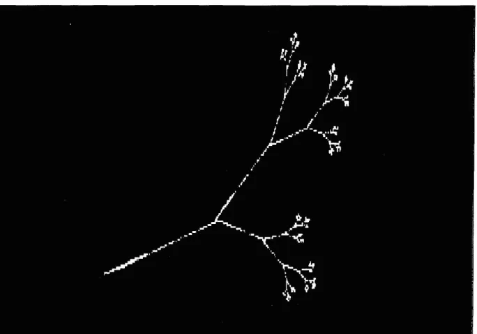
The real power of this method cannot be demonstrated with strictly self-similar objects because these can be generated as quickly ifnot faster in a variety of more direct ways. However where an object is composed of much less obvious self-affine copies of itself, then the method is truly magical. We will demonstrate this for three objects, all tree-like shapes which are much more realistic than those shown in the previous sections of this chap-ter. First we show a simple twig which involves three transformations of the original object into two which reflect branching and one which reflects the stem. Figure 2.20 illustrates the transformations in terms of the first level of recursion and the final object after some 10,000 iterations. This twig is adapted from Peitgen, Jurgens and Saupe (1992) who show that itdoes not matter what the actual object is which initiates the process because whatever object it is, it will be scaled down to a point at the resolution of the screen before it is plotted; thus it is only thetransformationsof the point which govern the form of the object which is eventually generated. We might begin with the Taj Mahal or some equally elaborate object but as long as the transformations of the object are those shown in Figure 2.20, a twig will be the ultimate form which we see as an approximation to the fractal attractor.

Figure 2.20.

Three transformations defining a twig.

poss-Size and Shape, Scale and Dimension 89

Figure 2.21. Realistic trees based on four and five transformations.

ible to see the Koch curve transform itself into a fern and vice versa. In fact this 'morphogenesis' can be animated for the interpolated values are like those used by animators in the process of 'in-betweening'; an example is given by Peitgen, Jurgens and Saupe (1992).

Figure 2.22. Barnsley's fern.

Size and Shape, Scale and Dimension 91

2.9 Idealized Models of Urban Growth and Form

This has been a long but necessary chapter, long because it is essential to have at least a rudimentary knowledge of all the key developments in frac-tal geometry and fracfrac-tal forms before we begin our applications to urban form, necessary because it puts us into a position to begin speculating on the geometrical properties of city shapes and how we might see them as fractals. In the rest of this book we will be dealing with two basic properties of urban form which involve, on the one hand, boundaries to urban devel-opment, and on the other hand, the growth of cities, their size, shape and density as we might perceive them in terms of fractal clusters. Weare, however, already in a position to say something about how strictly self-similar fractal forms compare with idealized city shapes which have been suggested down the ages and which we briefly reviewed in Chapter 1. As a conclusion to this chapter, we will present some of these speculations.

The Koch curve was used by Mandelbrot (1967) as an idealized model of a coastline because its fractal dimension was close to that estimated for the west coast of Britain (D = 1.262), while its geometric properties nicely captured the way a coastline might repeat its form at different scales. In fact, as we will show in Chapter 5, urban boundaries are somewhat like coastlines in terms of the extent to which they fill space, and thus the Koch curve might also be a good model for a city boundary. There is, however, an obvious but perhaps serendipitous comparison we can draw here. Man-delbrot (1983) noted that the slightly distorted H tree such as that shown in Figure 2.13(b) reminded him of the 17th century fortress works of the French Engineer Vauban, and in the same way the Koch island might be likened to the regular fortifications suggested by Renaissance scholars as encompassing ideal cities and actually implemented in many new towns such as Naarden and Palma Nuova (Morris, 1979; Rosenau, 1983). In Figure 2.23, we show a selection of ideal town plans produced during the Renaiss-ance in Europe and echoing the classical ideals of Greek architecture and urban design as portrayed for example by Vitruvius.

Figure 2.23. Idealized plans: fortified Renaissance towns and Koch islands (from Morris, 1979).

suburbs by a regular patterns of radial roads. These features are even clear for the ideal towns shown in Figure 2.23.

Our second example also relates to the Koch curve. In Chapter 1, we dealt with the Radburn layout of residential housing in which it was possible to visit any place alongside the branches of roads servicing the area without crossing any of these roads. Such layouts were shown in Figure 1.19 and we discussed their properties in terms of the H tree in an earlier section of this chapter. Arlinghaus and Nysteun (1990) have suggested that fractals such as the Koch forest (Figure 2.3) and the Cesaro-Peano sweep curve (Figure 2.7) might be used as designs which 'maximize' the amount of lin-ear space for mooring boats in a marina. They illustrate the idea using the Cesaro-Peano design which we show in Figure 2.24 where they speculate that the elaborate nature of the mooring is more likely to coincide with the distribution of preferences in the related population than a design based on routine mooring along a waterfront. Moreover, as the amount of boat mooring is also increased dramatically by such space-filling designs, the density of development would be greater and costs per unit of development would likely be lower for each participant in the scheme.

Size and Shape, Scale and Dimension 93

Condominiumpod

In<lltlllip

Figure 2.24. Maximizing linear frontage using the Koch forest (from Arlinghaus and Nysteun, 1990).

L

K-o

K-1

K-2

K-3

(2.18)

(2.43) similar designs as Sierpinski carpets although in this case, the design is a dendritic form rather than that of an object into which holes are punched. We will refer to this then as a Sierpinski tree in the spirit of Mandelbrot. Itis easy to see that this tree is formed by tiling the initiator with five copies of itself, each scaled by one third the original size of the initiator. Thus using equation (2.19) the dimension is D=log (5)/log (3)=1.465. In Figure 2.25 we show three ways of presenting this idealized tree. In 2.25(a), we show the tree as a strictly self-similar fractal in which we form the attractor by tiling an aggregate unit, a square, by five smaller squares at each level of hierarchy. This is the same way we introduced Sierpinski's gasket; it represents the way we might measure the dimension of this fractal ifwe were approximating its form at different levels by changing the scale on which we were viewing and measuring it.

However, in Figure 2.25(b), we show the dendrite as a spanning tree at each level of the hierarchy. Itis from this figure that we might measure the perimeter of the fractal. Using equation (2.16) withNk

=

5kand rk

=

r/3k, assuming the length of each diagonal of the unit square at k

=

0 to be '~2, and that there are four diagonal spans to the perimeter of each square at the appropriate level, then the perimeter of the entire tree at level k would be given as

Lk

=

Nkrk

=

4'-12

(~r

The third way to examine the Sierpinski tree is as a growing fractal and this is shown in Figure 2.25(c). In this case, we now have a fixed scale r and a varying yardstick or 'radius'Rkat scalek.Now the mass of the fractal

can be measured as its number of partsNk where this number is growing

as the scale k of the tree gets larger. Then

N

k

=

(~kr

=

Rfr

D,

Equation (2.43) is of the same form as equation (2.31) which is the relation-ship between mass and linear scale for a growing fractal. In short, this is the relation that we are seeking and which we will exploit from Chapter 7 on when we develop real versions of the Sierpinski tree as the skeleton on which most cities develop.

Noting that the fixed scalerof the growing fractal is 1/27=3-3

, then the perimeter can be calculated for each scale kas (4"1/2/27)5k _{where we again}

use the four diagonal spans as the perimeter of each basic unit whose side is 1/27 of the unit square. This is a reasonable model of a growing dendrite although its construction is somewhat different from those trees presented in an earlier section. It is easy to use IFS to generate the tree for like the Sierpinski gasket, its only transformations are scaling and translation. There are five transformations and the coefficients are given as aj

=

dj

=

1/3 for

all i; bj

=

Cj= 0 for all i;el =11

=

Iz

=

e3

=

0;ez

=

13

=

e4

=

14

=

2/3; and es

=

Size and Shape, Scale and Dimension 95

Figure 2.26. Generating Sierpinski's tree using IFS.