A Comparative Analysis of Computer Based Forecasting
Models Used In Stock Exchange Prediction
1
Onu, Fergus U. (Ph.D),
2Uche-Nwachi, Edward O.,
3Anigbogu, Gloria N.
1, 2
Department of Computer Science, Ebonyi State University. Abakaliki. Ebonyi State, Nigeria.
3 Department of Computer Science, Nwafor Orizu College of Education, Nsugbe. Anambra State, Nigeria
ABSTRACT
It is difficult to successfully forecast stock market prices to achieve the best result with minimal input. That’s
because stock price forecasting is a complex process that depends on both known and unknown factors. This
paper evaluates the different computer based forcasting models and presentes a comparative analysis of the use
of these models in stock exchange prediction. The paper used data for the period between January 2010 to
December 2015, and used each of The Markov model, Neuro-fuzzy system, Data mining, Neural Network,
ARIMA model, Moving average, Genetic algorithm, and Random walk forecasting models to reveal how they
have been used in stock market price forecasting. Also a combination of Neural Network and ARIMA models
were used to form a hybrid model and the outcome of the two methods were compared. R statistical program
was used to decompose the time series values into trends, seasonal and random components which gave a
deeper insight into the behaviour of the stock exchange market. The result obtained from the different forcasting
models including the hybridized models showed that the hybridized models gave the most accurate prediction in
stock exchange market forcast compared to the single models.
Keywords:
Forecasting models, prediction, Stock market price, Hybrid Model,
1.0 INTRODUCTION
The ultimate aim to maximize profit has prompted forecasters to come up with new and more accurate prediction formula or models. Forecasting is an attempt to envisage how the outcome of future event will occur, hence aid decision makers in making better decision. Forecasts are made not only to make profit but also to reduce risk and errors. Forecasting also facilitates better planning for future event and unforeseen circumstances. Stock exchange forecasters over the years have developed models to help in forecasting the best stock price with minimal error. It is difficult to make accurate prediction because of volatile markets and the fluctuation of stock prices. Forecasting stock market price is difficult because the fluctuations the market volatility needs to be captured and implemented by the model
The fluctuations in the market price affect investments from investors, as a result developing or comparing exiting forecasting models to facilitate the process of making better informed and accurate investment decisions is important not only to the forecasters but also to the investors. There exist many forecasting techniques such as Markov model, Neuro-Fuzzy system, Data mining, Neural Network, ARIMA model, linear and multi-linear regression, genetic algorithm, random walk, buy and hold strategy that are used for forecasting of future values.
These forecasting models can be grouped into prediction
techniques and time series analysis.(Prediction
Techniques – Neural Network, Hidden Markov Model, ANFIS, Genetic Algorithm, Data mining )(Time series
Analysis- Random work, Moving Average Regression, Method, ARIMA)
This research focuses on comparing some of the available stock market computer based forecasting model, and then recommending the most suitable computer based forecasting model that could be used in forecasting stock market prices with minimal error. Accuracy results of the forecasting models used in this study are present in Table 2 below.
The contribution of this study is a comparable analysis of the different stock market forecasting model, and the recommendation of the most suitable stock market forecast model with higher accuracy. Stock markets are some of the most important aspect of today’s global economy. Countries around the world depend on stock exchange for economic growth
A stock market is a public market for trading the company’s stock and derivative at an approved stock price. Stock market allows companies to buy and sell their shares. The shares price varies depending on the demand and supplies of shares. The price will increase when the demand is high and the share price decrease when the share is heavy to sell. This type of transaction is called trading and the companies, which are permitted to do the trading are called “listed companies” (Preethi & Santhi , 2012).
Available online: https://edupediapublications.org/journals/index.php/IJR/ P a g e | 605 do. There was no official share that changed hands
(Beattie, 2016). John Castaing in 1698 founded the arguably the oldest of the world’s major stock exchanges the: London Stock Exchange. John began to organize the market in Jonathan’s Coffee-house using a simple list of stock and commodity prices.
The New York Stock Exchange (NYSE) formed in 1792 is arguably the oldest, and most well known of all the American stock markets. The NYSE was formed when two dozen stockbrokers from New York City had the idea to organize what was then disorganized and chaotic method of trading. The NYSE continues to grow rapidly, and today lists 2,330 companies with a total capitalization of nearly $18.8 trillion(cite source). In 1849 the American Stock Exchange or Amex was formed. The Amex played an important role in the financial and business transactions associated with the mining industry in the 19th century. Amex expanded its niche role in 1921 to include companies that did not meet the strict standards of the NYSE. In 1998, the NASDAQ bought over Amex and it continued its history of niche market player, specializing in derivatives ad stock options. In January 2008, NYSE acquired the American Stock Exchange for $260 million in stock. The oldest stock exchange in Asia known as Bombay Exchange known as Munbai was formed 1875. In 2016, almost 34.7 million shares of stock worth $9.8 billion (USD) were traded monthly on the Bombay Stock Exchange. The National Association of Securities Dealers Automated Quotation, or NASDAQ was established in 1971 was the first exchange to recognize the role of electronics stock trading. The networks of computers running the NASDAQ allow it to be the most efficient stock exchange in the world (Money-Zine, 2016).
2.0 LITERATURE REVIEW
The prediction of stock market price that is effective and accurate is daunting and challenging task. In this paper, the literature review on the application of different forecasting techniques used in forecasting stock market price. Predicting stock index with traditional time series analysis has proven to be difficult; an artificial neural network may be suitable for the task.
Artificial neural network (ANN) technique is one of data mining techniques that is gaining prominence and gaining rapid acceptance in the business area due to its ability to learn and detect relationship among nonlinear variables. It allows for deeper analysis of large data sets, especially data that have tendency to fluctuate within short period of time ( Ayodele, Ayo, Adebiyi, and Otokiti, 2012). ANN is capable of extracting useful information from large set of data, and it can also be used for classification, predication and recognition ( Preethi & Santhi , 2012).
The uniqueness of ANN is its ability to relate the input to the output data set through a non-linear relationship. The
output value can be determined from the input values which have to be transformed using activation functions. The most crucial step involved in this training a neural network which required trainer to perform at optimum best ( Chakravarthy and Sunil,2016). ANN represents one of the widely used soft computing techniques for stock market forecasting. Trafalis used feed-forward ANN to forecast the change in the S&P(500) index (Hassan, Baikunth, and Kirley, 2017)
Hui-Kuang and Kun-Huang (2010) utilized neutral
network because of their capabilities in handling nonlinear relationship and also implement a new fuzzy time series model to improve forecasting. Among the several forecasting techniques developed to stock price prediction artificial neural networks model is very popular because of its ability to learn patterns from data and infer solution from unknown data (Adebiyi, Adewumi and Ayo, 2014).
The ability of neural network to learn the behavior the series when properly trained and because of their non-parametric approach have become popular in the world of forecasting. If stock market prices/returns fluctuations are affected by their recent historic behavior, neural network which can model such temporal stock changes can prove to be better predictors. The changes in a stock market can then be learned better using networks which employ a feedback mechanism to cause sequence leaning (Vaisla and Bhatt, 2010).
Autoregressive integrated moving average (ARIMA)
model also known as Box-Jenkins model was introduced by Box and Jenkins in 1970 is composed of set of activities for identifying, estimating and diagnosing ARIMA models with time series data. The model is most prominent methods in financial forecasting and it has shown efficient capability to generate short-term forecast. The ARIMA model creates small forecasting errors in longer experiment time period. The models constantly out-perform complex structural models in short-term forecast. The future value of a variable is a linear combination of past values and past errors. ARIMA models are known to be robust and efficient in financial time series forecasting especially short-term prediction than even the most popular artificial neural networks models (Adebiyi, Adewumi and Ayo, 2014). This model is fitted to the time series analysis data to predict future points in the series. ARIMA models are applied in some situations where the data show evidence of fluctuations also where an integrated part of the model can be applied to remove the fluctuation ( Preethi and Santhi,2012).
It also provides an effective means of predicting future values of the time series. Most time it is desirable to smooth a time series and thus eliminate some of the more volatile short-term fluctuations (Newberne,2006). An important characteristic of exponential smoothing is that weights are applied to the past values. Weights can be set so that the most recent and most relevant observations are given more weight than those observations further in the past. The exponential smoothing technique used in the Holt-Winters method requires a smoothing constant set in the range 0 <α <1. This constant is used to apply weights to the observations. The optimal value of smoothing constant varies based on the time-series data in question. It is usually set between 0.05 and 0.03, although it is possible to estimate α by reducing the sum of squared prediction errors (National Statistics United Kingdom,2005). The Holt-Winter smoothing algorithm tends to be more accurate for accounts that trend in one direction over time. It is a double exponential smoothing method that is appropriate for series with a linear trend and no seasonal variations. It is an extension of simple exponential smoothing method that was initially designed for time series with no trend nor seasonal pattern. The Holt-Winters model contains two important components; an exponentially smoothing constant (E, α) and a trend component (T,β) (Ortiz,2015).
The moving average method uncover the patterns and relationships and extract values of other variables from the database to predict the future values of other variables through the use of time series data. The moving average model offers advantage of reducing fluctuations and obtaining trends with a fair degree of accuracy ( Preethi, and Santhi, 2012).
Hidden Markov Model is a signal detection model which has established in 1966. The model assumes that observation sequences were derived by hidden state sequence which is a discrete data and satisfy the first order of a Markov process. HMM was developed from a model for a single observation to a model for multiple observations. HMM has been applied in different fields such as speech recognition, biomathematics, and financial mathematics. (Nguyen,2016)
Hidden Markov Model was first invented in speech recognition, but is extensively used to forecast stock market data. Markov process is a stochastic process where probability at one time is only conditioned on a finite history, being in a certain state at a certain time. Markov chain is “Given the present, the future is independent of the past” Hidden Markov Model (HMM) is a form of probability finite state system where the actual states are not directly observable. They can only be estimated using observable symbols associated with the hidden state. At each time point, the HMM produces
a symbol and changes a state with certain probability. In HMM, for a given observation sequence, the hidden sequence of states and their corresponding probability values are found. HMM gives a better accuracy than other models. Using the given input values, the parameters of the HMM (λ) denoted by A,B and π are found out. An HMM can be defined as λ =(S,O,A,B,π) where S={s1,s2,….sN} is a set of N possible states.
O={o1,o2,…oM} is a set of M possible observation
symbols. A is an NxN state Transition Probability Matrix (TPM). B is an NxM observation or Emission Probability Matrix (EPM). π is an N dimensional initial
state probability distribution vector (Kavitha,
Udhayakumar, and Nagarajan, 2013).
Nguyen (2016) used HMM with both single and multiple observations to forecast economic regimes and stock price. HMM can be used to not only with multiple observations data (open, low, high, close price), but also in single observation data (close price) to predict future close price. Since HMM can used either/both the single and multiple observations to predict stock’s close prices, we can compare the two methods to see which method had a better result.
In Hassan and Nath study, HMM was used to forecast the price of airline stocks. The goal is to predict the closing price on the next day based on the opening price, the closing price, the highest price and the lowest price today. The performance of the HMM is similar to that of artificial neural networks (ANN). (Hong, and Pitcan, 2015).
Neuro-Fuzzy networks can be used to forecast and investigate stock price behavior. Fuzzy sets theory is a theory used for taking steps in an uncertainty. In Adaptive Neuron-Fuzzy Inference System (ANFIS), a model such as “Takagi-Sugeno” is used to designing a pattern. It could be presumed that the fuzzy inference system has two inputs X1,X2 and an output Z. For first
order Sugeno, the equation of IF-THEN is as follows: IF(X1, is A1) AND (X2, is B1) THEN f1 = P1 X1 +q1 X2+r1
IF(X1, is A2) AND (X2, is B2) THEN f2 = P2 X1 +q2 X2+r2
In the calculation of “First order Sugeno”, the degree of
membership variable of X1 in membership variable of A1
are multiplied by the degree of membership variable of X2 and in membership function B1 and the product is
deemed as a first Linear regression Weight(W1).
Furthermore, in the second equation, the degrees of membership variable X1 in the membership function of
A2, is multiplied by the degree of membership variable
of X2 in the membership function of B2 and the product is
deemed as the second Linear regression Weight(W2). As
a result, the weighted average F1 and F2 is deemed as an
ultimate output (Z) which is calculated as follows Z= W1 x f 1 + W 2 x f2
Available online: https://edupediapublications.org/journals/index.php/IJR/ P a g e | 607 Takagi and Sugeno fuzzy model was used by Chang and
Chen study to forecast Taiwan Stock exchange price deviation. (Abbasi, and Abouec, 2008).
Genetic Algorithm is a heuristic function for optimization, where the extreme of the function cannot be established analytically. Genetic Algorithms promote “survival of the fittest”. This type of heuristic has been applied in many different fields, including construction of neural networks and finance. Genetic Algorithm (GA) has been applied in stock market and many finance fields. There have been numerous attempts to used GA for acquiring trading rules, both for Foreign Exchange Trading and S&P500 market ( Lin, Cao, Wang, and Zhang, XXx). Genetic algorithms can be used to predict the values of stock bases on the biological phenomenon of natural selection and natural evolution. It makes use of bio-inspired operators such as mutation, crossover and selection. The first step involves the creation of “population” of randomly generated strings of 0s and 1s. This population is evaluated at every “generation” based on the fitness function which is used to calculate the fitness of every individual in the population that is being
evaluated. The fitness is usually the optimum value.
Once the fitness has been evaluated, the chromosomes that have better chance to reproduce are passed onto the next generation. This is followed by cross-over and mutation. Crossover refers to the process of randomly selecting a cross site and then swapping genes of the two parent chromosomes along the cross site. After the crossover operation, mutation is performed which involves changing the string by changing relevant bits from 1s to 0s or vice-versa. This is done to generate a variance in the population ( Chakravarthy and Sunil,2016).
The random walk model is frequently used as a model for the stock market quotations. For this particular model all the predictions are equal to the last observed value, and the confidence intervals are higher as the forecast horizon is expanding (Rusu and Rusu, 2003). In random walk, the stock market price changes have the same distribution and these are independent of each other. The stock prices are fluctuating and financial status of a gambler can be modeled as random walk. Random walks can be used in many fields such as ecology, economics and psychology. The random walk explain the observed behavior of processes in these areas (Preethi and Santhi, 2012).
Hybrid Model
Previous studies have shown that the accuracy of forecasting model increases when the several models are combined. Many studies have proposed the use of hybrid of hybrid models, such as ARIMA, ANN. Zheng in his study used a hybrid model based on three sets of data: data on wolf sunspot, data canduan lynx, and Great
Britain Pounds exchange ratio, the America dollar to model the wasting result. Pie and Lim in their study also used a hybrid model consisting of Support Vector Machine (SVM) and peremptory model to predict daily stock (Pirzad And Porannejad ,2014)
3.0 METHODOLOGY:
Stock data used in this study are historical monthly stock prices obtained from finance yahoo website. The data set consisted of trading day from 1st January 2010, to December 30th 2015(monthly data). The data is collected from historical stock prices were obtained from
published stock prices on the internet
(https://finance.yahoo.com. ). The stock Exchange data consisted of date, closing price, low price, high price, adjusted closing price and volume.
In this study, the closing price is chosen to represent the price of the index to be predicted. The closing price is chosen because it reflects all the activities of the index in a trading day.
Training data period for the long-term is from January 1, 2010 to December 30, 2015. The monthly index value resulted into 72 values in the time series data. During this period 60 values (months) were selected for the training, and 12 values (months) were selected for the testing data. We use the ts() function in the tseries library in the R programming language to convert the raw data into reversed formatted data into a frequency of 12 monthly time series. Three components (Trend, Seasonal and Random) are aggregated into time series in the time series in R. In order to study and investigate the behavior of each component in greater details, we used decompose ( ) function defined in the tseries library in R. After the decomposition, each of the components of the time series and their respective behavior were scrutinized closely. Some robust forecasting techniques were applied to the data to critically analyze the accuracy of each of the forecasting methods that we have applied.
DECOMPOSTION RESULTS
Figure 1: Stock Exchange Index time series (January 2010- December 2015)
Figure 2: Decomposition of Stock Exchange index time series into trend, seasonal, and random components
The overall time series for the Stock Exchange index for the period of January 2010 to December 2015 is shown in figure1. It can be seen that the time series had an increasing trend till the curve exhibited a small downward fall during the mid part of 2015. Figure 2 shows the decomposition results of the time series of Figure 1. The three components of the time series are
shown separately to facilitate proper visualization of their respective behavior.
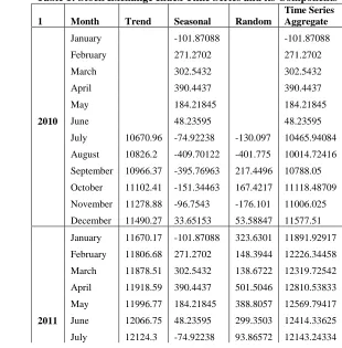
The numerical values of the time series data and its three components are contained in Table 1 below. The trend and the random components are not available for the period of January 2010 to June 2010 and also for the period of July 2015 to December 2015. The non-availability of data for trend for the stated periods is due to the fact that in the computation of trend, long term data. In order to compute trend figures for January 2010-June 2010 we need time series data from July 2009 to December 2009. Similarly, to compute the trend values for July 2015 to December 2015, time series data from January 2016 to July 2016 are needed. Due to the non-availability of data, it is also impossible to calculate the random values for January 2010 to June 2010, and July 2015 to December 2015.
It can be seen in Table 1 that the aggregate time series is the sum of the trend, seasonal and random components, and that the seasonal components remains constant for the same month over the same period. Hence the missing seasonal component can be figured out but the missing trend values cannot be figured out. As a result, it is impossible to compute the aggregate time series of these specific months.
Table 1: Stock Exchange Index Time Series and its Components
1 Month Trend Seasonal Random
Time Series Aggregate
January -101.87088 -101.87088
February 271.2702 271.2702
March 302.5432 302.5432
April 390.4437 390.4437
May 184.21845 184.21845
2010 June 48.23595 48.23595
July 10670.96 -74.92238 -130.097 10465.94084
August 10826.2 -409.70122 -401.775 10014.72416
September 10966.37 -395.76963 217.4496 10788.05
October 11102.41 -151.34463 167.4217 11118.48709
November 11278.88 -96.7543 -176.101 11006.025
December 11490.27 33.65153 53.58847 11577.51
January 11670.17 -101.87088 323.6301 11891.92917
February 11806.68 271.2702 148.3944 12226.34458
March 11878.51 302.5432 138.6722 12319.72542
April 11918.59 390.4437 501.5046 12810.53833
May 11996.77 184.21845 388.8057 12569.79417
2011 June 12066.75 48.23595 299.3503 12414.33625
Available online: https://edupediapublications.org/journals/index.php/IJR/ P a g e | 609 August 12185.41 -409.70122 -162.178 11613.53041
September 12252.83 -395.76963 -943.678 10913.38209
October 12306.8 -151.34463 -200.448 11955.00709
November 12316.25 -96.7543 -173.817 12045.67917
December 12328.31 33.65153 -144.401 12217.56041
January 12383.78 -101.87088 351.0051 12632.91417
February 12481.39 271.2702 199.4094 12952.06958
March 12648.1 302.5432 261.3956 13212.03875
April 12800.82 390.4437 22.36838 13213.63208
May 12889.21 184.21845 -679.976 12393.4525
June 12966.98 48.23595 -135.123 12880.0925
2012 July 13055.07 -74.92238 28.53113 13008.67875
August 13152.16 -409.70122 348.3829 13090.84166
September 13255.03 -395.76963 577.8696 13437.13
October 13379.72 -151.34463 -131.92 13096.45542
November 13560.9 -96.7543 -438.569 13025.57667
December 13758.89 33.65153 -688.399 13104.14208
January 13947.24 -101.87088 15.21422 13860.58334
February 14122.67 271.2702 -339.447 14054.49292
March 14264.83 302.5432 11.16263 14578.53583
April 14437.41 390.4437 11.94588 14839.79958
May 14667 184.21845 264.3528 15115.57125
2013 June 14939.22 48.23595 -77.8576 14909.59833
July 15160.5 -74.92238 413.9578 15499.53542
August 15331.57 -409.70122 -111.555 14810.31333
September 15504.33 -395.76963 21.1088 15129.66917
October 15655.17 -151.34463 41.9238 15545.74917
November 15794.45 -96.7543 388.7168 16086.4125
December 15941.06 33.65153 601.9526 16576.66416
January 16065.25 -101.87088 -264.533 15698.84584
February 16204.92 271.2702 -154.477 16321.71333
March 16379.97 302.5432 -224.857 16457.65625
April 16536.56 390.4437 -346.161 16580.84292
May 16686 184.21845 -153.047 16717.17125
2014 June 16810.51 48.23595 -32.1447 16826.60125
July 16923.53 -74.92238 -285.308 16563.3
August 17060.08 -409.70122 448.0758 17098.45458
September 17190.47 -395.76963 248.2005 17042.90084
October 17297.89 -151.34463 243.973 17390.51834
November 17404.27 -96.7543 520.7197 17828.23542
December 17491.21 33.65153 298.2097 17823.07125
February 17594.36 271.2702 267.0706 18132.70083
March 17539 302.5432 -65.4232 17776.12
April 17518.78 390.4437 -68.7079 17840.51583
May 17525.65 184.21845 300.8149 18010.68333
2015 June 17504.55 48.23595 66.72572 17619.51167
July -74.92238 -74.92238
August -409.70122 -409.70122
September -395.76963 -395.76963
October -151.34463 -151.34463
November -96.7543 -96.7543
December 33.65153 33.65153
4. RESULT AND DISCUSSIONS
The seasonal components of the Stock Exchange Index are positive during the period of February to June and negative from July to November. The seasonal component value is at minimum on the month of August, while the maximum seasonal component is in the month of April. The trend component value decreased in the month of February 2015 and March 2015, then increased slightly in April 2015, but decreased again in May 2015. It is most likely the decrease could continue in the few months after May. The random component values shows fluctuations. The time series can be feasible for forecasting since the trend component being the major component of the time series shows a decrease pattern within the months of February 2015 to May 2015.
The study makes attempt to compare the accuracy of the most popular forecasting models, and then propose a more accurate hybrid forecasting model consisting of ARIMA and ANN.
R statistical program was used to build the forecasting models to test the historic time series aggregate data. The built Neural Network, ARIMA, Polynomial Fit Model Seasonal Fit Model, Advanced Linear Model and Hybrid forecasting models’ accuracy were measured using the historic time series aggregate monthly data.
The different forecasting methods that were applied on the time series data of the Stock Exchange Index. The seven forecasting techniques that were proposed and their forecasting accuracy are listed and discussed below.
The time series data of the Stock Exchange Index from January 2010 to December 2015was used to compute its trend and seasonal components. Forecasting for the yearly indices for the year 2015 is made on the basis of time series data from January Error in forecasting 2010 till the end of the previous year for which forecast is
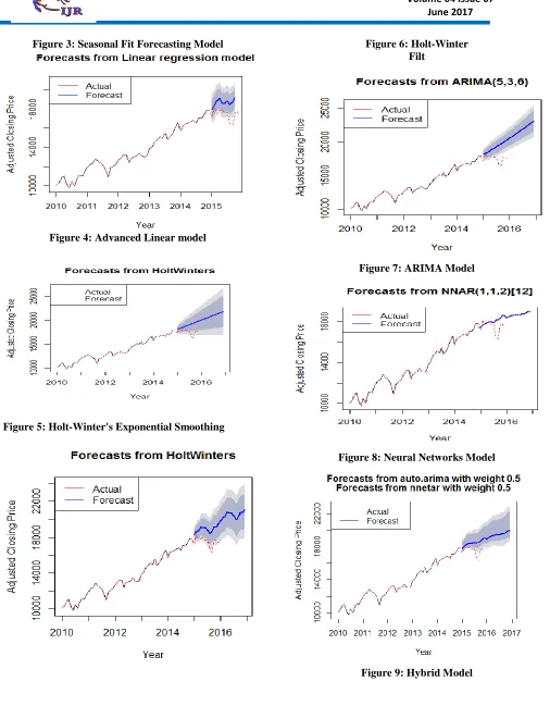
made is also computed. Errors in forecasting are also computed. The time series the of Stock Exchange yearly indices from the year January 2010 to December 2014 is use to compute, its seasonal and trend components. The training data is computed from the time series of the Stock Exchange indices from the January 2010 to December 2014 using R statistical program. We use the following models: Neural Network, Arima, Seasonal Fit, Advanced Linear HoltWinter Exponential Smoothing, Holt-Winter Filter and Hybrid with a forecast horizon of one year to compute the forecast value for the seven models. The forecasting accuracies of the seven models are graphically illustrated in figures 3 to 9 below.
Available online: https://edupediapublications.org/journals/index.php/IJR/ P a g e | 611 Figure 3: Seasonal Fit Forecasting Model
Figure 4:Advanced Linear model
Figure 5: Holt-Winter's Exponential Smoothing
Figure 6:Holt-Winter Filt
Figure 7:ARIMA Model
Figure 8:Neural Networks Model
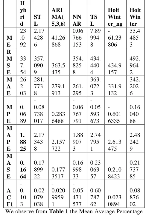
Table 2: Forecasting Models Accuracy computation Results H yb ri d ST L ARI MA( 5,3,6) NN AR TS L Holt Wint er_ng Holt Win ter M E 23 .0 92 2.17 428 6 41.26 868 0.06 766 153 7.89 994 8 -61.23 806 33.4 485 3 R M S E 33 7. 54 357. 090 9 363.5 435 354. 825 8 434. 440 4 434.9 157 492. 964 2 M A E 26 2. 03 281. 773 8 279.1 913 261. 295 363. 072 3 331.9 132 342. 202 6 M P E 0. 06 89 -0.08 738 017 0.283 6488 -0.06 767 791 -0.05 593 673 -0.601 6335 0.16 040 88 M A P E 1. 88 25 2.17 343 8 2.157 722 1.88 907 3 2.74 795 1 2.613 475 2.48 242 9 M A S E 0. 16 64 0.17 899 22 0.177 3517 0.16 998 33 0.23 063 57 0.210 8423 0.21 737 85 A C F1 -0. 10 3 0.02 079 038 -0.020 9959 1 -0.05 471 577 0.60 787 62 -0.023 0894 0.08 876 02
We observe from Table 1 the Mean Average Percentage
Error (MAPE) of all the forecasting models is relatively small, and that the Hybrid forecasting model had the
lowest MAPE of 1.8825 and the lowest Mean Absolute
Scale Error (MASE) of 0.1664.
As mentioned earlier the Stock Exchange dataset was divided into training and test set. Training set was used to train forecasting models and test set was used to measure forecasting model performance. Forecasting performance was measured in terms of Mean Absolute Error (MAE), Mean Absolute Percentage Error (MAPE),
Root Mean Square Error (RMSE),Mean Error
(ME),Relative Mean Absolute Error (RMAE), Mean
Percentage Error (MPE), Mean Absolute
Scaled Error (MASE), First-Order Autocorrelation
Coefficient (ACF1).
ANNs are data-driven model and consequently, the underlying rules in the data are not always apparent. Also, the buried noise and complex dimensionality of the stock market data makes it difficult to learn or re-estimate the ANN parameters (Kim & Han, 2000).
It is also difficult to come up with an ANN architecture that can be used for all domains. In addition, ANN occasionally suffers from the overfitting problem (Romahi and Shen, 2000).
Neural Network results are unstable. The neural network functions are Block Box function. The rules of operations are completely unknown. Back propagation networks can be take long time to train the large amount of data. Unlike a regression model, ARIMA model do not support the stationary time series data (Preethi and Santhi, 2012).
The limitations listed above could be overcome by the proposed a hybrid model that combines ARIMA model and neural network to improve the accuracy of the stock market index forecasting.
CONCLUSION
In this work, we have analyzed the Stock Exchange index time series during the period of January 2010 to December 2015. R statistical program was used to decompose the time series values into trend, seasonal, and random components. The decomposition of the time series provided a deeper insight into the behavior of the Stock Exchange index time series. Using the decomposed result, we applied seven forecasting models for forecasting the index value of the Stock Exchange sector for two years (2015 and 2016).
The results obtained from the different forecasting model showed that the hybrid model had the least MAPE and MASE, consequently proved to be the most accurate model for forecasting Stock Exchange when compared to the previously listed forecasting models.
REFERENCES
Abbasi,E and Aboue, A ( 2008). Stock Price Forecast by
Using Neuro-Fuzzy Inference System. World
Academy of Science, Engineering and Technology 46 2008
Adebiyi, A.A, Adewumi,A.O and C. K. Ayo (2014). Stock Price Prediction Using the ARIMA Model. UKSim-AMSS 16th International Conference on Computer Modelling and Simulation
Adebiyi A, A., Ayo C, K., Adebiyi, M, O., and Otokiti, S, O (2012). Stock Price Prediction using Neural Network with Hybridized Market
Indicators. Journal of Emerging Trends in
Computing and Information Sciences. VOL. 3, NO. 1, ISSN 2079-8407
Beattie, A. (2016) .The Birth Of Stock Exchanges.
Available online: https://edupediapublications.org/journals/index.php/IJR/ P a g e | 613 http://www.investopedia.com/articles/07/stock
exchange-history.asp
BeBusinessed, (2016).History of The Stock Market.
Retrieved from
http://bebusinessed.com/history/history-of-the-stock-market/
Chakravarthy,S and Shraddha, S. (2016). A Comparative Analysis of Different Machine Learning Algorithms Used in Predicting Stock Market Prices. International Journal of Advanced Research in Computer and Communication Engineering. Vol. 5, Issue 11, November 2016. Hassan, R, Baikunth, N and Kirley, M (2007). A fusion
model of HMM, ANN and GA for stock market forecasting. Expert Systems with Applications 33 (2007) 171–180
Hong C, Y and Yannik Pitcan, Y. (2015). An introduction to the use of hidden Markov models for stock return analysis. Retrieved
from
http://jcyhong.github.io/assets/intro-hmm-stock.pdf
Hui-Kuangyu, T. and Huarng, K (2010). A Neural network-based fuzzy time series model to improve forecasting. Elsevier, 2010, pp: 3366-3372.
Jing Tian (). Economic Value of Stock Return Forecasts: An Assessment on Market Efficiency and
Forecasting Accuracy Retrieved from.
.https://editorialexpress.com/cgi-bin/conference/download.cgi?db_name=ESAM 07&paper_id=108
Lin, L, Cao,L, Wang, J and Zhang, C. (xxx). The Applications of Genetic Algorithms in Stock Market Data Mining Optimisation
Kavitha, G. Udhayakumar, A and Nagarajan, D (2013). Stock Market Trend Analysis Using Hidden
Markov Models. Retrieved from
https://arxiv.org/ftp/arxiv/papers/1311/1311.47 71.pdf
Kim, K. J., and Han, I. (2000). Genetic algorithms approach to feature discretization in artificial neural networks for the prediction of stock price
index. Expert Systems with Applications, 19,
125–132.
Money-Zine (2016). Stock Market History. Retrieved
from
www.money-zine.com/investing/stocks/stock-market-history/ National Statistics United Kingdom. (2005).
Methodology of the Experimental Monthly Index of Services. Retrieved January 27, 2017, from
http://www.statistics.gov.uk/iosmethodoloqy/ defauIt.asp
Newberne, J, H. (2006). Holt-Winters Forecasting: A Study of Practical Applications for Healthcare. Army-Baylor University Graduate Program in Healthcare Administration
Nguyet Nguyen (2016).Stock Price Prediction using
Hidden Markov Mode. Retrieved from
https://editorialexpress.com/cgi-bin/conference/download.cgi?db_name=SILC2 016&paper_id=38
Ortiz, L. R (2015). The Accuracy Rate of Holt-Winters Model with Particle Swarm Optimization in Forecasting Exchange Rates. Journal of Computers. Volume 11, Number 3
Pirzad, A and Porannejad, M (2014). Stock Exchange Index Prediction Using Hybrid Models. Indian J.Sci.Res. 7 (1): 186-193, 2014. ISSN: 0976-2876 Preethi, G and B.Santhi (2012). Stock Market
Forecasting Techniques: A Survey. Journal of
Theoretical and Applied Information Technology. Vol.46. No 1
Romahi, Y., & Shen, Q. (2000). Dynamic financial forecasting with automatically induced fuzzy
associations. In Proceedings of the 9th
international conference on fuzzy systems (pp. 493–498).
Vaisla, K.S and A.K. Bhatt (2010). An Analysis of the Performance of Artificial Neural Network Technique for Stock Market Forecasting. International Journal on Computer Science and Engineering. Vol. 02, No 06, 2104-2109
Wen-Chih Tsai An-Pin Chen(2002 ). Using Hidden
Markov Model for Stock Day Trade Forecasting.
Retrieved online on 20/01/2017 from