Classification of heterodimer interfaces using docking models and construction of scoring functions for the complex structure prediction

(1)

Advances and Applications in Bioinformatics and Chemistry

Dove

press

open access to scientific and medical research

Open Access Full Text Article _{O R i g i n A L R e s e A R C h}

Classification of heterodimer interfaces using

docking models and construction of scoring

functions for the complex structure prediction

Yuko Tsuchiya1

eiji Kanamori2,3

haruki nakamura4

Kengo Kinoshita1,5 1_{institute of Medical science,}

University of Tokyo, Tokyo, Japan;

2_{Biomedicinal information Research}

Center, Japan Biological informatics Consortium, Tokyo, Japan; 3_hitachi

software engineering Co., Ltd., Yokohama, Japan; 4_{institute for Protein}

Research, Osaka University, Osaka, Japan; 5_{Bioinformatics Research}

and Development, JsT saitama, Japan

Correspondence: Yuko Tsuchiya human genome Center, institute of Medical science, The University of Tokyo, 4-6-1 shirokanedai, Minato-ku, Tokyo, 108-8639, Japan

Tel +81 3 5449 5131 Fax +81 3 5449 5133 email [email protected]

Abstract: Protein–protein docking simulations can provide the predicted complex structural models. In a docking simulation, several putative structural models are selected by scoring functions from an ensemble of many complex models. Scoring functions based on statistical analyses of heterodimers are usually designed to select the complex model with the most abundant interaction mode found among the known complexes, as the correct model. However, because the formation schemes of heterodimers are extremely diverse, a single scoring function does not seem to be sufficient to describe the fitness of the predicted models other than the most abundant interaction mode. Thus, it is necessary to classify the heterodimers in terms of their individual interaction modes, and then to construct multiple scoring functions for each heterodimer type. In this study, we constructed the classification method of heterodimers based on the discriminative characters between near-native and decoy models, which were found in the comparison of the interfaces in terms of the complementarities for the hydrophobicity, the electrostatic potential and the shape. Consequently, we found four heterodimer clusters, and then constructed the multiple scoring functions, each of which was optimized for each cluster. Our multiple scoring functions were applied to the predictions in the unbound docking.

Keywords: classification of heterodimers, prediction of complex structures, scoring functions, protein–protein docking, CAPRI

Introduction

Many biological functions of proteins occur through specific recognition among protein molecules. Knowledge of protein–protein interactions, particularly three-dimensional structural information of protein–protein complexes, is crucial for understanding the biochemical and physiological functions of proteins.1–3_{Recently, the number of}

tertiary structures of protein complexes has been increasing by the efforts of structure biologists; however, it is still smaller than that of known protein–protein interactions.4–6

Therefore, the precise prediction of protein complex structures is required for further experimental studies. A protein–protein docking simulation is one of the popular approaches to predict protein complex structures.7–9

Docking procedures generally consist of two main steps, a sampling step and a subsequent scoring step. A large number of complex models are generated in the former step. The problem of searching the high dimensional conformational space to create a collection of complex models was studied by various research groups.10–19_However,

there are still several issues to overcome, such as the introduction of conformational flexibility in the generation of near-native models for targets with large conforma-tional changes.9,20,21_{In the latter step, the selection of near-native models is achieved}

Advances and Applications in Bioinformatics and Chemistry downloaded from https://www.dovepress.com/ by 118.70.13.36 on 19-Aug-2020

For personal use only.

Number of times this article has been viewed

(2)

Tsuchiya et al Dovepress

with a scoring function from the many complex models generated in the former step. The various scoring functions that are presently available evaluate complex models in terms of the surface complementarity22,23_{along with the}

electrostatic filter,10,11,24–26_{the atomic contact energy (ACE)}27

or the statistical potentials based on the pairs of interacting residues,28–30_{including hydrogen bonds and van der Waals}

interactions. However, the selection of correct solutions is not easily performed in the structure predictions of many different heterodimers.9,21

As previous studies have pointed out,1–3_{various types}

of heterodimer complexes exist not only in biological func-tions and three-dimensional structures, but also interaction modes. For example, there are heterodimers with electrostatic dominant interfaces, those with hydrophobic dominant interfaces, and those without interfaces but with high or low shape complementarity. In contrast, the scoring functions based on the statistical analysis of heterodimer interactions are usually designed to select the complex models with the most abundant interaction mode in the known complexes, and thus a single scoring function will not be enough to evaluate the diverse protein–protein interfaces. In addition, the identification of the interaction modes, ie, the classification of heterodimer complexes, was usually performed based on the interface characters observed in experimentally determined structures of heterodimers. However, to make a native dimer structure, the information about the difference between noninteracting sites and interacting sites will be more important because even a weak interface can be a native interface if no other better interfaces exist.

Several pioneering works have already proposed the multiple scoring functions optimized for each type of protein function.10,31–33_{However, they focused only on two types:}

enzyme-inhibitor and antibody–antigen type complexes. The other heterodimers, such as those related to signal transduc-tion and gene transcriptransduc-tion and translatransduc-tion, were classified as other types.32,34_{This is probably because the small numbers}

of known complex structures make it difficult to find the functional similarities between these heterodimers and to categorize them. Thus, the classification of heterodimers by using information other than that of protein functions will facilitate the construction of the multiple scoring functions.

In this study, we addressed the problem of selecting the correct solutions from the many complex models in the scoring step, by considering the various features of the heterodimers. First, we classified the native interacting sites by considering decoy structures, where the search for the parameters of the scoring functions to discriminate

the near-native and the decoy models was carried out. As a scoring function, we used a linear combination of the weighted values of three complementarity scores for the hydrophobicity, the electrostatic potential, and the shape at the protein–protein interface.35_{This function indicates the total}

degree of complementarities for the three surface features over the interfaces. The four heterodimer clusters were found according to our classification scheme. Four scoring functions were then constructed as multiple scoring functions where each function was optimized for each heterodimer type.

Materials and methods

Training dataset

native heterodimer complexes

The X-ray crystal structures of heterodimers, according to the biological units described in the header of the Protein Data Bank (PDB),36_{which have 2.5 Å or better resolution}

and consist of two protein chains with more than 30 residues and a sequence identity lower than 85% by FASTA program,37

were extracted from the PDB in April 2006. Among these structures, 122 representative heterodimers from each SCOP family class38_{were finally selected. These entries are listed in}

Supplementary Tables 1 and 2. We referred to these experi-mentally determined complexes as the native complexes.

Complex models generated by the sampling method

Up to 500 models for each heterodimer entry were generated by using our sampling method39_{in the bound–bound docking}

where the structures of two protomers derived from the complex structure were used. This method generates complex models by optimizing an objective function, which evaluates the shape complementarity of the molecular surfaces of two component protomers by evaluating the angle of the normal vectors at the vertices on their molecular surfaces, and the sequence conservation of the surface residues calculated by the evolutionary trace (ET) analysis,40_{when required.}

The sequence conservation information was not used for generating the complex models in this section, because there are the case where such information is not effective in indentifying the interacting region, and the case where a suf-ficient number of homologous sequences cannot be obtained to calculate the sequence conservation.39_{However, we used}

conservation information to construct one of the two test datasets, as described in the next section. The optimization of the objective function was accomplished by using a genetic algorithm in combination with Monte Carlo sampling. The final models were selected so that each model had a ligand-rmsd (L-ligand-rmsd) larger than 3.0 Å from any other models.

(3)

Analysis of diverse heterodimer interfaces Dovepress

Note that the smaller protomer in a complex structure is referred to as a ligand protein, and the larger protomer as a receptor protein. The rmsd is the root mean square deviation of one structure from another structure. The ligand-rmsd is the rmsd between the ligand proteins in two complex models when the receptor proteins are superimposed. Since we could not obtain any correct solutions, in other words, near-native models for the 43 entries, by the above sampling procedure, we carried out Monte Carlo sampling of the complex models by starting from the native structure to obtain the conformations around the native conformations, and we used these conformations as the near-native models. The Monte Carlo sampling was also performed so that each model had an optimized objective function and an L-rmsd

smaller than 10.0 Å from the native complex. It should be noted that in the CAPRI experiments, the submitted models with an L-rmsd smaller than 10.0 Å from the correct answer are judged as the successful models.41,42_{Then, all models}

were energy minimized by the myPresto program.43_{In one}

entry, no model was successfully minimized due to many clashes. Therefore, we decided to exclude this entry from the dataset. Consequently, both near-native models and decoy models could be prepared for 121 heterodimer entries. The total numbers of the near-native and the decoy models in the 121 heterodimer entries are 404 and 60,238, respectively.

The optimized objective function39_{was used as an}

indicator of the quality of a complex model concerning the area and the shape complementarity in the contact region.

Table 1 The test dataset: the CAPRi targets

Target (PDB ID)a _{Component proteins}b _Near-nativec _Decoyd _Highest

ranke

Scoring

functionf

Characters of the native interface

T12 (1ohzg₎ _{Cellulosomal scaffolding}

cohesin/dockerin xylanase domain

1 29 8 f_c₃ Almost flat, Hydrophobic and

electrostatic complementary interface

T18 (-) endo-1, 4-B-xylanase/its inhibitor TAXi

1 29 1 fc 4 highly concave and convex,

highly shape and no hydrophobic complementary interface T21 (1zhih₎ _{Origin recognition complex}

subunit1/regulatory protein sir1

1 29 2, 1 f_c₁, f_c₂ nonglobular complex, highly electrostatic and modestly shape complementary interface T25 (2j59i₎ _{ADP-ribosylation factor1/Rho}

gTPase-activating protein 10 ARF-binding domain

1 297 103 f_c₃ Almost flat, Hydrophobic and shape complementary interface

T26 (2hqsj₎ _{Peptidoglycan-associated}

lipoprotein/tolb

7 112 7 fc3 Concave and convex, hydrophobic

and shape complementary interface

Notes:a_{The target identity and the PDB iD of the native heterodimer complex. The PDB iD of T18 is unknown.}b_{information for the component proteins.}c_{The number of}

near-native models used in the test. d_{The number of decoy models used in the test.}e_{The highest rank of the near-native model.}f_{The scoring function that made the highest}

rank of the near-native model. g_{Carvalho et al.}62h_{hou et al.}63i_{Menetrey et al.}64j_{Bonsor et al.}65

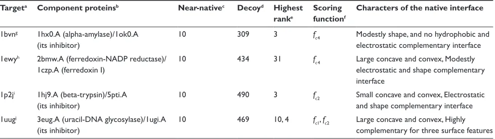
Table 2 The test dataset: the unbound–unbound pairs of the four heterodimer entries

Targeta _{Component proteins}b _Near-nativec _Decoyd _Highest

ranke

Scoring

functionf

Characters of the native interface

1bvng _{1hx0.A (alpha-amylase)/1ok0.A}

(its inhibitor)

10 309 3 f_c₄ Modestly shape, and no hydrophobic and electrostatic complementary interface 1ewyh _{2bmw.A (ferredoxin-nADP reductase)/}

1czp.A (ferredoxin i)

10 434 31 f_c₄ Large concave and convex, Modestly electrostatic and shape complementary interface

1p2ji _{1hj9.A (beta-trypsin)/5pti.A}

(its inhibitor)

10 490 3 f_c₂ small concave and convex, electrostatic and shape complementary interface 1uugj _{3eug.A (uracil-DnA glycosylase)/1ugi.A}

(its inhibitor)

10 469 10, 4 f_c₁, f_c₂ Large concave and convex, highly complementary for three surface features

Notes:a_{The PDB iD of the native complex of the training heterodimer entry.}b_{PDB iDs and chain iDs of the monomeric structures of the component proteins and their}

information. c_{The number of near-native models used in the test.}d_{The number of decoy models used in the test.}e_{The highest rank of the near-native model.}f_{The scoring}

function that made the highest rank of the near-native model. g_{Wiegand et al.}66h_{Morales et al.}61i_{helland et al.}67 j_{Putnam et al.}59

(4)

Since the magnitude of the objective function differs entry by entry, the ratio of the optimized objective function of the model to that of the native complex, called the “relative docking-score”, was considered, where the objective func-tions of the native complexes were calculated in the same way as that in the sampling method. The relative docking-score = 1.0 means that the complex model had an interface as good and large as that in the native complex. In this study, we defined the complex models with an L-rmsd smaller than 10.0 Å from the native complex and a relative docking-score higher than 0.95 as the near-native models.

heterodimers used in developing scoring functions

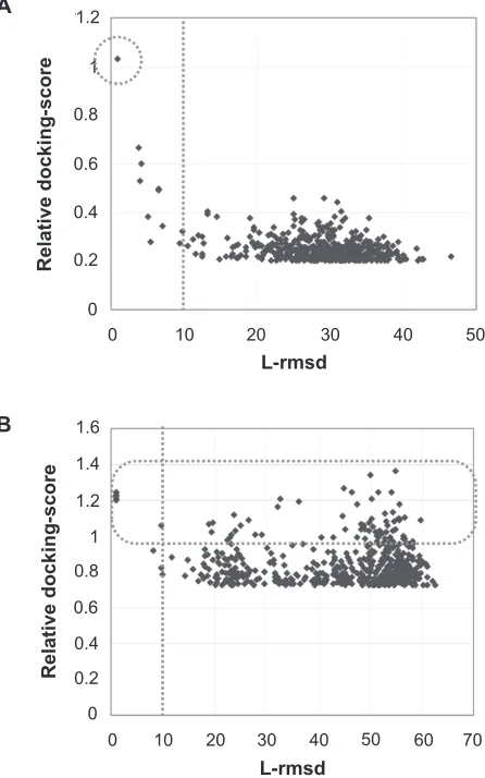
The 121 heterodimer entries were divided into two groups: one contained 47 entries, and another contained 74 entries. In the former 47 entries, the complex model with the largest relative docking-score was the near-native model. On the other hand, in the latter 74 entries, the model with the largest relative docking-score was not the near-native model, and there were some “false positive models”, which we defined as the complex models with 10.0 Å or greater L-rmsds from the native complexes and with relative docking-scores higher than 0.95. For the latter 74 entries, scoring functions that evaluate the complex models by regarding factors other than the contact area should be required to select the correct solutions. We considered that the number of false positive models is related to the difficulty in the selection of the correct solutions, and that it may be advantageous to develop multiple scoring functions by using the latter cases. Thus, we examined the number of false positive models in the set of complex models for the 121 heterodimer entries.

In the 47 heterodimer entries, no false positive model was obtained, as shown in Figure 1A, which provides an example of the relation between the L-rmsd and the relative docking-score of each complex model. The native complexes of these entries are entangled, as in a swapping dimer or a dimer with a loop wound around it. The regions corresponding to the entangled loops in the complex state are usually flexible or disordered in the monomer state, and these regions will be fixed or ordered when the complex is formed. In the bound–bound docking, these entries will not yield any false positive complex models due to their tangles. On the other hand, in the unbound–unbound docking it will be difficult to generate the near-native models due to their flexibility. This is because the monomeric structures of the protomers are used, which may have flexible loops or disorder regions. Thus, in these entries, the near-native models will be selected based only on their contact area without ranking of the complex

1

A _1.2

0.8 0.6 0.4 0.2 0

0 10 20 30 40 50

L-rmsd

0 10 20 30 40 50 60 70

L-rmsd

1.2 1.4 1.6

1 0.8 0.6 0.4 0.2 0

Relative docking-score

B

Relative docking-score

Figure 1 A) An example of the heterodimers that do not need ranking of complex models to select the near-native models. The scatter plot shows the relation between the L-rmsd from the native complex and the relative docking-score in each model, in the heterodimer entry. As this plot shows, this entry, the heterodimer between chains B and F of 1or7 (RnA polymerase sigma-e factor and its negative regulatory protein),68

has no model with a 10.0 Å or greater L-rmsd and a higher relative docking-score than 0.95. B) An example of the heterodimers that need ranking of complex models for the selection of the near-native models. This heterodimer, chains A and B of 1ksh (arf-like protein 2 and 3′,5′-cyclic phosphodiesterase delta-subunit),69_{has many models with}

large L-rmsds and high relative docking-scores.

models by the scoring functions. These 47 entries are listed in Supplementary Table 1.

The other 74 heterodimer entries have at least one false positive decoy, as shown in Figure 1B, where there are many false positive models with various L-rmsds. The native complexes of these entries have either convex and concave surfaces or almost flat surfaces in the interacting regions. These entries may require the evaluation functions other than the contact area to select the correct solutions, and therefore, they could be suitable for the development of scoring functions. Consequently, we decided to use these 74 heterodimer entries, listed in Supplementary Table 2, as the training entries to construct the scoring functions. For each

(5)

of these heterodimers, 491.8 complex models, including 4.4 near-native models, were obtained on average.

Test datasets

The CAPRi targets

For the CAPRI targets T12, T18, T21, T25, and T26, the complex models were generated from two initial struc-tures in unbound–bound forms (targets T12, T18, and T25) or in unbound–unbound forms (targets T21 and T26) by using our sampling method, where the ET scores were included in the objective functions.39_{We used the models with an L-rmsd}

smaller than 10.0 Å from the native complexes and with any relative docking-scores as near-native models (summarized in Table 1). It should be noted that we did not set the thresh-old of the relative docking score in the determination of the near-native models for the test datasets. This is because the structures of the component protomers of the test targets and those of the corresponding native complexes were deter-mined under different crystallization conditions, and thus a comparison of the scores of the complex models for the test targets with those of the native complexes is not significant.

The unbound–unbound pairs of the heterodimer entries

Six heterodimers, which have the monomeric structures of the two component protomers stored in the PDB, were found in the training dataset. We performed the unbound– unbound docking from the monomeric structures of these entries by our sampling method without ET scores so that up to 500 complex models were generated for each entry. Four entries were available for this test because the other two entries yielded no model with an L-rmsd smaller than 10.0 Å from the native complexes due to the conformational changes of the loop structures involved in the protein–protein interaction. All four of the entries had 10 or more models with L-rmsds smaller than 5.0 Å. Therefore, we chose 10 models with the largest values of the optimized objective functions among the complex models with L-rmsds smaller than 5.0 Å for each target as the near-native models. The other models with L-rmsds smaller than 10.0 Å were not used in this test. The information for these entries is summarized in Table 2.

scoring function

A scoring function was defined as a linear combination of weighted complementarity scores for the hydrophobicity, the electrostatic potential, and the shape on the molecular surfaces of the protein–protein interface. The basis of the complementarity calculation was originally developed for

the classification and analyses of homo-oligomer interfaces in our previous study.35_{First, a Connolly surface}44_consisting

of triangular polygons was constructed for each protomer. Next, the hydrophobicity calculated by the Ooi–Oobatake method,45_{and the electrostatic potential obtained by solving}

the Poisson–Boltzmann equation numerically with the SCB program46_{were mapped onto each vertex on the Connolly}

surface. The shape of the surface was also considered using the average curvatures at each vertex.47_{The interacting region}

on the surfaces was defined as a set of pairs of vertices from different surfaces with a distance shorter than 3.0 Å. Then, the complementarity scores, H_cmp, E_cmp, and S_cmp for the hydropho-bicity, the electrostatic potential and the shape, respectively, were defined as the ratio of the number of complementary vertex-pairs for the hydrophobicity (N_hyd, hydrophobic and hydrophobic), the electrostatic potential (N_ele, opposite sign of the potential) or the shape (N_shape, convex and concave), respectively, to the total number of vertex-pairs exist-ing in the interface, N_total, as follows: H_cmp =N_hyd N_total, E_cmp=N_ele N_total and S_cmp=N_shape N_total. It should be noted that we used the two indices of the shape complementarity of the interfaces in this study. One is the shape complemen-tarity calculated by the objective function in the sampling step, which is used to choose complex models that have no or few crashes, moderately large areas, and almost continu-ous interfaces, and to eliminate poor models. Another is the

S_cmp that represents the degree of the shape complementarity against the interface, which is used to compare the different complex models in terms of the shape complementarities of the interfaces. The parameters to define the complementary vertex-pairs for the three surface features were optimized in conjunction with changing the distance cut off in the definition of the interacting region, from 1.0 Å in the original study35_{to 3.0 Å, so that the difference between the}

comple-mentarity scores of the energy-minimized and nonenergy-minimized models was nonenergy-minimized. Since the optimization of the parameters was performed independently of this study, it will not be discussed further.

Finally, the degree of complementarities, COMP, was defined as follows:

COMP = W_h × H_cmp + W_e × E_cmp + W_s × S_cmp (1)

where the weight parameters, W_h, W_e, and W_s, are normal-ized so that W_h2₊W_e2₊W_S2 ₌₁_._{The weight parameters} were optimized by introducing the subparameters w₁, w₂, and w₃, so that W_h=w W1 , We =w W2 and Ws=w W3

where W = w1 +w +w

2 2 2

3

2_{to ensure the constraint of}

W_h2₊W_e2₊W_S2 ₌₁_._{The subparameters were changed}

(6)

from -100 to 100 at intervals of 1. Thus, 8, 120, 600 (= 2013 - ₁₎

weight combinations, the combinations of w₁, w₂, and w₃, were considered, where 1 is (w₁, w₂, w₃) = (0, 0, 0). The values of

W_h, W_e, and W_s ranged from -1.0 through 1.0, respectively.

search for the successful weight

combinations

The highly successful weight combinations in the selection of near-native models were searched among all of the pos-sible weight combinations, to classify the heterodimers and then to construct the multiple scoring functions, as follows.

Conversion of the three-dimensional weight combinations into the two-dimensional space

The three-dimensional weight combinations were con-verted into the two-dimensional space of two angles,

the zenith and azimuth angles in polar coordinates, where the radius = 1, the zenith angle was the angle between the

W_s-axis and the line from the origin to the considered point, and the azimuth angle was that between the positive

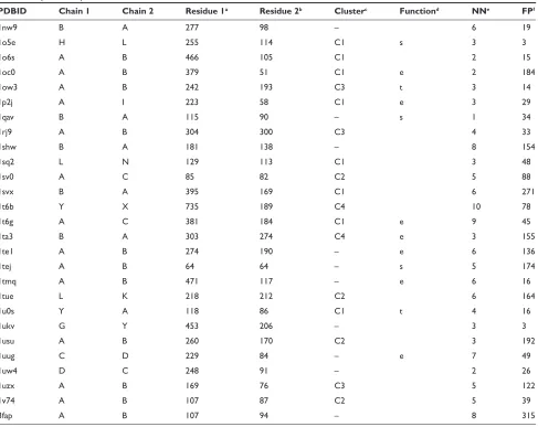
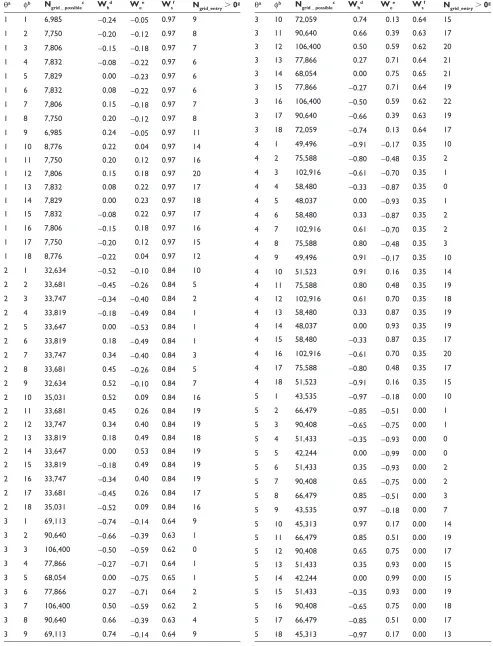
W_h-axis and the line from the origin to the considered point, projected onto the W_h-W_e plane. The two-dimensional space was separated into 162 grids at intervals of 20 degrees as shown in Figure 2. We considered two more grids, which correspond to (W_h, W_e, W_s) = (0, 0, 1) and (W_h, W_e, W_s) = (0, 0, -1), because when the zenith angle is 0 or 180, namely

W_s= 1 or -1, respectively, the azimuth angle cannot be defined. It should be noted that this weighing scheme did not yield equal density of weight combinations. Therefore, these 164 grids contained different numbers of weight combinations, as shown in the third column of Supple-mentary Table 3.

180

160

140

120

100

θ

ϕ

80

60

40

20

0

Wh We

1

–1

–1 0 0

1

1 0

0 0

–1 1

C1 C2 C3 C4

–180 –160 –140 –120 –100 –80 –60 –40 –20

0 ₂₀ ₄₀ ₆₀ ₈₀

100 120 140 160 180

2 3 4 5 6 7 8 9 10 11 12 13 14 15 16 17 18

grid 1

2 fc4 fc1

fc3 fc2

3 4 5 6 7 8

9 –1

0

1

Ws

(0,0,1) (0,0,–1)

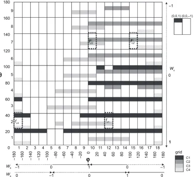
Figure 2 The distribution of the grids with high foccrs in each cluster. The grids with foccrs higher than 5.0 in the entries belonging to each cluster are colored based on the

color bar on the bottom-right corner, where “C1”, “C2”, “C3” and “C4” mean Clusters 1, 2, 3 and 4, respectively. The outside grids with (0, 0, 1) and (0, 0, -1) are those corresponding to (Wh, We, Ws) = (0, 0, 1) and (Wh,We,Ws) = (0, 0, -1), respectively. The Wgrids in the grids surrounded by black dotted-lines were defined as the multiple

scoring functions, where the grids with fc1, fc2, fc3 and fc 4 were selected from Clusters 1, 2, 3 and 4, respectively. The serial numbers of each grid for the zenith (θ ) and azimuth

(φ ) angles, respectively, are also shown on the axes of the both angles, which are assigned at intervals of 20 degrees, respectively.

(7)

An occurrence frequency of the successful weight combinations in a grid

In each training entry, for each weight combination, the COMP values of all complex models were calculated, and the complex models were ranked in the order of the COMP values. Then, an occurrence frequency, f_occr(θ, φ), of the weight-combinations that could rank the near-native models in the top 10 was calculated in each grid according to the following Equation,

f N N N occr grid entry grid possible total entry ( , ) ( , ) ( , ) _ _ _ θ φ θ φ θ φ = N

N_{total possible}_{_} (2)

where N_{grid_entry}(θ, φ) was the number of weight combinations that could rank at least one near-native model in the top 10 in each grid, and N_{grid_possible}(θ, φ) was the number of all of the possible weight combinations belonging to each grid, which was shown in the third column of Supplementary Table 3. Because N_{grid_possible}(θ, φ) differs grid by grid as described above, N_{grid_entry}(θ, φ) was normalized by N_{grid_possible}(θ, φ) in Eq. 2, to avoid under- or overestimation in the calculation of the f_occr. The “θ ” and “φ ” were the serial numbers of each grid for the zenith and azimuth angles, respectively, and they were assigned at intervals of 20 degrees on the axes of the both angles as shown in Figure 2. It should be noted that a prediction is generally regarded as “acceptably” successful, when the correct solutions are ranked within the top 10. This criterion is also adopted in the CAPRI experiment.41,42

(N_{total_entry}/N_{total_possible}) was set to correct the differences in

the degrees of difficulty in ranking the near-native models in the top 10 between different entries. N_{total_entry} was the summation of the N_{grid_entry}(θ, φ)s in all grids. N_{total_possible} was the summation of the N_{grid_possible}(θ, φ)s in all grids, namely

N_{total_possible}= 8,120,600. If (N_{total_entry}/N_{total_possible}) is 1, then all

weight-combinations can rank the near-native models in the top 10. When (N_{total_entry}/N_{total_possible}) is considerably smaller than 1, only a few weight combinations can rank the near-native models highly. This indicates that the selection of the near-native models in the latter case is more difficult than that in the former case. The high f_occr(θ, φ) indicates that the weight combinations existing in the grid have high possibilities of success in the selection of near-native models.

Results and discussion

Classification of the heterodimer entries

We first tried to classify the 74 heterodimers to construct the multiple scoring functions that select the near-native models from many decoy models, as summarized in the flowchart in Supplementary Figure 1 where the whole procedures for

constructing the multiple scoring functions are shown. The classification was performed based on the discriminative characters between near-native models and decoy models, which were found in the calculation of the f_occr(θ, φ) for each grid in each entry, as follows.

As shown in the seventh column of Supplementary Table 3, the numbers of entries with N_{grid_entry}(θ, φ) larger than 0 were very diverse. It suggests that there are no major grids in which the weight parameters can succeed in selecting near-native models in many entries, and therefore, the classification will be required. Thus, the 74 training heterodimer entries were classified based on the f_occr(θ, φ)s in all 164 grids in each entry, by the clustering method of program R,48_{where the}

Euclidean distances between the 164-dimensional vectors of the f_occr(θ, φ)s were used as the distances between entries. The distances between the clusters were then calculated by Ward’s method. This clustering method divided the 74 training heterodimer entries into two groups clearly, where one group was also separated into two clear clusters, but another was not divided. We investigated the grids where the entries belong-ing to each group had f_occr higher than 5.0, and found that the separation in the former group related to the grids with high

f_occr, as shown in Figure 2. We also found that the latter group might be separated into two clusters in the same manner as that in the former group. Therefore, we decided to classify the heterodimers into four clusters, Clusters 1 and 2 from one large group, and Clusters 3 and 4 from another large group, each containing 15, 12, 9, and 9 entries, respectively. It should be noted that we tried 1.0, 2.5, 5.0, and 7.5 as the f_occr criterion to define the distribution of the grids. When either 1.0 or 2.5 was used as the criterion, the difference between the distribu-tions in the two groups was unclear. On the other hand, some entries had no f_occr(θ, φ) higher than or equal to 7.5. Therefore, we used 5.0 as the criterion. The grids where at least one entry belonging to a cluster had the f_occr(θ, φ) higher than 5.0 were regarded as the “grids belonging to the cluster”, which were colored according to the color bar in Figure 2. Note that the grids could belong to two or more different clusters. The other 29 entries could not be classified as any clusters, because no weight-combination could rank the near-native models in the top 10, namely the f_occr(θ, φ)s in all grids were 0.

Our method succeeded in the selection of the near-native models in 45 entries (60.8% = 45/74), as described above. To investigate the performance of our method, we examined the performance of ZDOCK12_{in the bound–bound docking}

for the 74 training heterodimers. ZDOCK could include at least one complex model with the L-rmsd smaller than 10 Å from the native complex in the best 10 models, in 62 entries

(8)

(83.8% = 62/74). Because our criterion for a successful prediction is that at least one complex model with the L-rmsd smaller than 10 Å from the native complex and with the relative docking-score larger than 0.95 is ranked in the top 10, we calculated the relative docking-scores of the best 10 complex models generated by ZDOCK. We also tried 0.90 and 0.85 as the thresholds of the relative docking-score, because 0.95 might be a severe threshold for ZDOCK models which were not optimized for the objective functions by our sampling method. As the result, in 43 entries (58.1% = 43/74), at least one complex model could meet our criterion. For 0.90 and 0.85 thresholds, 52 (70.3% = 52/74) and 56 (75.7% = 56/74) entries could meet the criteria, respectively. Thus, the performance of our method was not very low, compared to that of ZDOCK in the bound-bound docking for our training dataset.

All of the grids with high f_occr(θ, φ)s in Cluster 1 had positive weights for the shape of the interface. This indicates that the shape complementarity was the most effective contributor in ranking the near-native models in the top 10. In other words, the shape complementarity was the “discriminator” of the near-native models from the other decoys. The discriminators in Clusters 2 and 3 were the complementarities for the electrostatic potential and the hydrophobicity, respectively. In Cluster 4, the weight of the shape contribution was positive; however, the weight of the hydrophobicity was negative. The informa-tion about these clusters is summarized in Table 3.

Construction of the multiple scoring

functions

Based on the classification results, the multiple scoring functions were constructed so that each function was

applicable to the selection of the near-native models in the heterodimer entries belonging to each cluster, as follows. First, we considered the respective averages of the three weight values corresponding to all weight-combinations belonging to each grid, as a representative weight-combination in each grid, which we designated as W_grid. Then, the near-native models were again selected by using the 164 W_grids for the training entries. Finally, four W_grids, each of which was a W_grid in a grid belonging to each cluster, were chosen so that the total number of successful entries in the selections by the four W_grids was maximized. Since there were cases where the near-native models in an entry could be ranked in the top 10 by two or more W_grids belonging to different clusters, the total number of successful entries by the four W_grids was counted as follows, to avoid overlaps in counting: the number of successful entries by a W_grid from Cluster 1 was counted, and then, among the failed entries by the W_grid from Cluster 1, the number of successful entries by a W_grid from Cluster 2 was counted. This procedure was iterated up to Cluster 4. The number of successful entries was counted for all of the possible combinations of the four W_grids from the four clusters. Consequently, we selected the four W_grids, with grids surrounded by the dotted-lines in Figure 2, as the multiple scoring functions, and desig-nated them as f_c₁, f_c₂, f_c₃ and f_c₄, from Clusters 1, 2, 3 and 4, respectively. The real weight values of the four W_grids are f_c₁: (W_h, W_e, W_s) = (0.34, 0.40, 0.84), f_c₂: (-0.27, 0.71, -0.64),

f_c₃: (0.74, 0.13, -0.64), and f_c₄: (-0.52, -0.10, 0.84), respectively. The total number of successful entries by the four W_grids was 33 (73.3% = 33/45), where 45 was the number of entries where the near-native models could be selected by any W_grids.

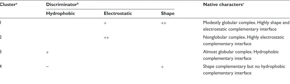
Table 3 Discriminator of the scoring function and characteristics of the native complexes in each cluster

Clustera _{Discriminator}b _{Native characters}c

Hydrophobic Electrostatic Shape

1 + ++ Modestly globular complex. highly shape and

electrostatic complementary interface

2 ++ nonglobular complex. highly electrostatic

complementary interface

3 + Almost globular complex. hydrophobic

4 – + shape complementary but no hydrophobic

Notes:a_{The cluster identity.}b_{The discriminator in each cluster. The terms “hydrophobic”, “electrostatic” and “shape” mean the complementarities for the hydrophobicity,}

the electrostatic potential and the shape, respectively. The “+” means that the corresponding weight had a positive effect on the selection of the near-native models. On the other hand, the “-” means that the weight did not contribute to the selection. The weight with “++” contributes significantly to the selection. c_{The characters of the native}

complexes of the entries classified as the cluster.

(9)

Classification results of heterodimers

in the training dataset

The heterodimers in our training dataset were classified based on the occurrence frequencies of the weight-combinations that could select the near-native models, as described above. Next, we tried to find the common characteristics in each cluster, and to investigate whether the classification results were related to the biological functions. To find the characteristics of the heterodimers, we examined the native complexes of the heterodimer entries from the aspects of the whole complex structures and the interface shapes by assessing them visually,49_{and the aspect of the interaction}

modes by checking the complementarity scores for the hydrophobicity, the electrostatic potential, and the shape at the interfaces, designated as H_cmp, E_cmp, and S_cmp, respectively. The common characteristics of the native complexes in each cluster are summarized in Table 3.

Common characteristics in Cluster 1

In 11 entries among the 15 entries belonging to Cluster 1, the interfaces of the native complexes have higher S_cmps than the average of the S_cmps in the 74 training entries (0.36). The

S_cmps in the other four entries are lower than the average, but are not very small (1m2t: 0.33, 1o6s: 0.34, 1sq2: 0.34, and 1t6g: 0.34). The overall structures of these 15 entries are modestly “globular”. Eight of them also have higher E_cmps than the average of the E_cmps (0.38). The entry in Figure 3A: the heterodimer of lysozyme C and antigen receptor V domain (1sq2),50_{which has a lower}_S

cmp (0.34) than the

average, shows that the proteins interact with each other by placing concave surfaces on convex surfaces. This suggests that shape complementarity is the dominant characteristic in this cluster. It corresponds to the discriminator in this cluster, namely the character of f_c₁.

Among the 12 entries in Cluster 2, 11 interfaces of the native complexes have higher E_cmps than the average (0.38), and their overall complex structures are “nonglobular”, as shown in Figure 3B: the heterodimer of the chaperone ATPase domain and the BAG chaperone regulator (PDB ID 1hx0,

E_cmp: 0.61),51_{where the electrostatically positive surfaces,}

colored blue, tightly interact with the electrostatically negative surfaces, colored red. Thus, the characteristic surface feature of the native interfaces in Cluster 2 could be the electrostatic complementarity, and it corresponds to the character of f_c₂.

The last entry, 1fxw, has lower complementarity scores for three surface features (H_cmp: 0.10, E_cmp: 0.28, and S_cmp: 0.29)

than the averages in the 74 training entries (0.16, 0.38, and 0.36), respectively. No significant characteristics were found for this example.

In seven of the nine entries classified in Cluster 3, the interfaces of the native complexes have higher H_cmps than the average (0.16). The interface shapes are either low convex and concave or almost flat. The whole complex structures are more “globular” than those in Clusters 1 and 2. The heterodimer of the GTPase domain of a signal recognition particle and its receptor (1rj9),52_{shown in Figure 3C, has}

an almost flat interface and a higher H_cmp (0.26) than the average, and resembles a homodimer interface. Thus, the characteristic surface feature of the native interfaces in this cluster could show the hydrophobic complementarity, which corresponds to the character of f_c3.

In the remaining two entries, one entry, 1clv, has lower complementarity scores for three surface features (H_cmp: 0.11,

E_cmp: 0.13, and S_cmp: 0.34), and the other entry, 1uzx, has lower H_cmp and S_cmp (H_cmp: 0.12, E_cmp: 0.55, and S_cmp: 0.29) than the averages (0.16, 0.38, and 0.36). Since the interface of the former entry consists of relatively highly convex and concave surfaces, this interface is considered to be similar to those of the entries belonging to Cluster 1. We could not understand why the latter case differed.

For all nine of the entries belonging to Cluster 4, the near-native models could be ranked in the top 10 by fewer weight-combinations than those in the other clusters. This indicates that the selection of the near-native models in this cluster was more difficult than those in the other clusters. The native interface of one entry has a steep shape, made of one loop structure, and those of the other five entries have smooth shapes, as shown in Figure 3D: the heterodimer of DNA polymerase III beta and delta chains (1jql).53_{In the}

other three entries, the native complexes have a few water molecules at the interacting regions. No characteristic of the native complexes was found in this cluster, and the features of these entries were similar to those of the entries that failed in the selection of the near-native models, described in the next section.

Failed entries in selecting the near-native models

Among the 74 training heterodimers, 29 were not classified as any clusters because no near-native model could be ranked in the top 10 by any weight combination. The native

(10)

A

B

C

D

E

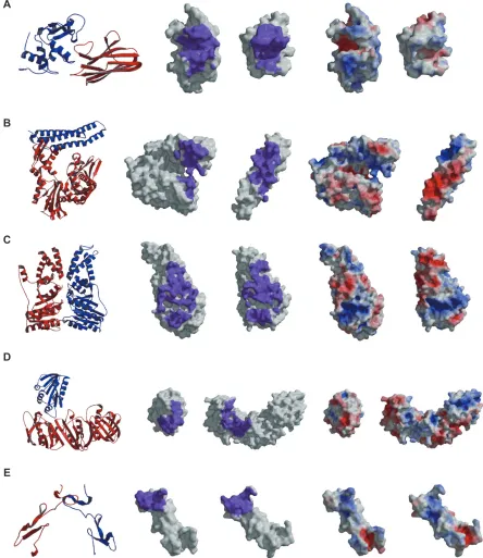
Figure 3 The characters of the native complexes of the heterodimer entries belonging to each cluster. For an entry in each cluster, the whole complex structure, the interface region colored purple, and the electrostatic potential mapped on the surfaces, where the negative and positive electrostatic potentials are colored red and blue, respectively, of the native complex are shown. The middle and left figures are shown in open-book view. A) An example in Cluster 1 (chains L and n of 1sq2). B) An example in Cluster 2 (chains A and B of 1hx1). C) An example in Cluster 3 (chains A and B of 1rj9). D) An example in Cluster 4 (chains A and B of 1jql). E) An example of the failed entries in the selection of near-native models (chains A and B of 1tej).

complexes in six entries have steep shapes at the interfaces and those in 17 other entries have smooth shapes or almost flat interfaces. In these 23 (= 6 + 17) entries, the protomers of the dimers could bind tightly with each other at different surface regions from the native interfaces, thus generating many

decoy models with high complementarity scores, as shown in Figure 3E: a disintegrin heterodimer (1tej).54_{In the other six}

entries, the native complexes have water or ligand molecules in the interacting regions. These native interfaces have lower complementarity scores than those expected. This is because

(11)

the protein–water and protein–ligand interactions were not considered in the calculation of the complementarities. Thus, the complementarity scores of the near-native models were also lower than those of other decoy models.

The many decoy models with high complementarity scores in the former 23 entries, and the low complementar-ity scores of the near-native models in the latter six entries made the correct selection difficult. Further optimization of the parameters or the introduction of other parameters in the calculation of interface complementarities might be required for these cases.

Biological functions of the heterodimers in each cluster

Among the 74 training entries, 19 enzyme-inhibitor complexes were included, as marked in Supplementary Table 2. We examined the clusters to which these enzyme-inhibitor complexes belonged, in order to investigate whether the classification results were related to the biological function. Twelve complexes were classified into four different clusters; five, two, two, and three entries belong-ing to Clusters 1, 2, 3, and 4, respectively. The other seven entries were not classified into any clusters because they failed in selecting the near-native models. In 14 of the 19 enzyme-inhibitor complexes, the native interfaces are formed through the interaction between the concave and electrostatically negative surface of the enzyme and the convex and electrostatically positive surface of the inhibitor, as shown in Figure 4B: the heterodimer of alkaline metal-loproteinase and its inhibitor (1jiw),55_{Figure 4C:}

alpha-amylase and its inhibitor (1clv),56_{and Figure 4D: endo}-_1,

4-beta-xylanase and its inhibitor (1ta3).57_{However, as}

these examples show, they have diverse depths and sizes of cavities and different ratios of molecular sizes between the enzyme and the inhibitor proteins. The other four enzyme-inhibitor complexes have both electrostatically positive and negative surfaces on each side of the interfaces, as shown in Figure 4A: the heterodimer of the TEM-1 beta-lactamase and its inhibitor protein II (1jtd).58_{In the remaining entry,}

1uug, the heterodimer of uracil-DNA glycosylase and its inhibitor,59_{which was not classified in any cluster and}

is shown in Figure 4E, the interface on the enzyme side is electrostatically positive, and that on the inhibitor is electrostatically negative. These observations indicate that the heterodimers with the same protein functions can have the different discriminative characters between the near-native and the decoy models, and also have the different dominant characters in their native interfaces.

It is widely accepted that transient and permanent complexes differ in terms of the type of interactions: the former complexes are often formed through salt bridges and hydrogen bonds, while the latter are formed through hydrophobic interactions.2_{Since the identification of transient}

complexes is difficult, we tried to find stable heterodimers by checking the primary citations of the native complexes of the training heterodimer entries, and also to find transient heterodimers by referring to the list of transient heterodimers by Nooren and Thornton.60_{We found 13 stable heterodimers}

and eight transient heterodimers. Among the latter transient heterodimers, five entries were included in their list, and the other three entries contained the domains with the same SCOP family identities38_{as those of the listed heterodimers.}

Both the stable and transient heterodimers were also classified as different clusters, as shown in Supplementary Table 2. It suggests that the discriminative interface characters are not common in transient complexes and in stable complexes, respectively, and moreover, there are no clear differences between the discriminative characters of transient complexes and those of stable complexes.

Thus, the clusters based on the discriminative interface characters between the near-native and the decoy models were independent from the types of biological functions of the heterodimers, and they were only related to the dominant characters of the native heterodimer interfaces.

scoring tests for unbound docking models

The multiple scoring functions were tested in the selection of the correct solutions from complex models, which were generated from the monomeric structures of component proteins of heterodimers. Two datasets were tested: one is the set of five CAPRI targets,8,21_{T12, T18, T21, T25, and T26, and}

the other is the set of four pairs of the monomeric structures for the four training heterodimer entries. For each target, both near-native and decoy models were generated by our sampling method from the monomeric structures in the unbound-bound form (T12, T18, and T25), and in the unbound–unbound form (T21, T26, and the four training entries). Note that the complex models for the CAPRI targets were generated by considering the sequence conservations by the ET method, as described in Materials and methods. Because we narrowed the search of complex models according to the result of the ET, we could not obtain a large number of models. Thus, the numbers of complex models in these targets were small and diverse. Although we did not calculate the number of false positive models for each target because the relative-docking scores could not be estimated for unbound docking models

(12)

A

B

C

D

E

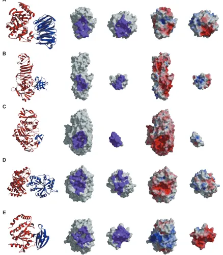
Figure 4 The characters of the native complexes of the enzyme-inhibitor type heterodimers. For the enzyme-inhibitor dimer classified as each cluster, the whole complex structure, the interface region colored purple, and the electrostatic potential mapped on the surfaces, where the negative and the positive electrostatic potentials are colored red and blue, respectively, of the native complex are shown. The middle and left figures are shown in open-book view. A) An example in Cluster 1 (chains A and B of 1jtd). B) An example in Cluster 2 (chains i and P of 1jiw). C) An example in Cluster 3 (chains A and i of 1clv). D) An example in Cluster 4 (chains A and B of 1ta3). E) An example of the failed entries in the selection of near-native models (chains C and D of 1uug).

as described before, the difficulty of the selection of the near-native models may differ target by target. In the scoring test, the rankings of the complex models were performed by each of the four scoring functions, and the prediction was considered to be successful when at least one near-native model could be ranked in the top three by at least one scoring

function. As a result, in two out of the five CAPRI targets and the two monomer pairs of the heterodimer entries, at least one scoring function could rank the near-native models within the top three. In the other three targets, the near-native models were ranked within the top 10. The characteristic surface features of the native interfaces also corresponded

(13)

to the characters of the successful scoring functions in these seven targets, as summarized in Tables 1 and 2 and shown in Supplementary Figure 2.

In the CAPRI target T25 and the monomer pair of 1ewy,61

no scoring function could rank the near-native models in the top 10. The highest ranks of the near-native models were 103 by f_c3 in T25 and 31 by f_c4 in 1ewy. The native complex of T25 has a hydrophobic interface with a complementary shape, and that of 1ewy has a modestly electrostatic and shape complementary interface. These features suggest that f_c3 for T25 and f_c2 or f_c4 for 1ewy are appropriate for selections of the near-native models. Thus, the characters of the scoring functions that made the highest ranks, also corresponded to the characteristic features of the native interfaces in these two entries.

Conclusion

In this study, we constructed the multiple scoring functions based on the classification of the diverse heterodimers. In the four clusters found in this study, Cluster 1 contained the largest number of entries (15 entries); however, there were few differences between the number of entries in Cluster 1 and those in the other clusters, 12, 9, and 9 in Clusters 2, 3, and 4, respectively. In other words, based on our classification scheme no major cluster with a dominant interaction mode was found. Therefore, we think that the multiple scoring func-tions constructed according to our classification scheme may have a better potential for selecting the near-native models of heterodimers than a single scoring function.

In an actual prediction, the selection of one scoring function appropriate for a given pair of protomers may be required. We consider that one possible approach to the selection is as follows; the COMP values of all complex models are calculated by each of the four scoring functions, and then, the Z-scores are estimated from the COMP values. The scoring function with the best Z-score can be the most appropriate scoring function. This approach succeeded in ranking the near-native models in the top 10 in two CAPRI targets (T21 and T26) and one monomer pair (1bvn) of our test datasets.

Acknowledgments

This work was supported by a Research Fellowship from the Japan Society for the Promotion of Science for Young Scientists to YT. KK was supported by a Grant-in-Aid for Scientific Research on Priority Areas from the Ministry of Education, Culture, Sports, Science and Technology of Japan (No. 17081003). HN was supported by a Grant-in-Aid for

Scientific Research on Priority Areas from the Ministry of Education, Culture, Sports, Science and Technology of Japan (No. 17017024). This work was also supported by the Japan Science and Technology Corporation for Strategic Japan-UK Cooperative Program to HN, KK, and YT. The authors report no conflicts of interest in this work.

References

1. Jones S, Thornton JM. Protein-protein interactions: a review of protein

dimer structures. Prog Biophys Mol Biol. 1995;1:31–65.

2. Jones S, Thornton JM. Principles of protein-protein interactions. Proc Natl Acad Sci U S A. 1996;1:13–20.

3. Lo Conte L, Chothia C, Janin J. The atomic structure of protein-protein

recognition sites. J Mol Biol. 1999;5:2177–2198.

4. Uetz P, Giot L, Cagney G, et al. A comprehensive analysis of

protein-protein interactions in Saccharomyces cerevisiae. Nature.

2000;6770:623–627.

5. Aebersold R, Mann M. Mass spectrometry-based proteomics. Nature.

2003;6928:198–207.

6. Russell RB, Alber F, Aloy P, et al. A structural perspective on

protein-protein interactions. Curr Opin Struct Biol. 2004;3:313–324.

7. Smith GR, Sternberg MJ. Prediction of protein-protein interactions

by docking methods. Curr Opin Struct Biol. 2002;1:28–35.

8. Janin J. Assessing predictions of protein-protein interaction: the CAPRI

experiment. Protein Sci. 2005;2:278–283.

9. Lensink MF, Mendez R, Wodak SJ. Docking and scoring protein

complexes: CAPRI 3rd Edition. Proteins. 2007;4:704–718.

10. Gabb HA, Jackson RM, Sternberg MJ. Modelling protein docking using shape complementarity, electrostatics and biochemical information.

J Mol Biol. 1997;1:106–120.

11. Heifetz A, Katchalski-Katzir E, Eisenstein M. Electrostatics in

protein-protein docking. Protein Sci. 2002;3:571–587.

12. Chen R, Li L, Weng Z. ZDOCK: an initial-stage protein-docking

algorithm. Proteins. 2003;1:80–87.

13. Dominguez C, Boelens R, Bonvin AM. HADDOCK: a protein-protein docking approach based on biochemical or biophysical information.

J Am Chem Soc. 2003;7:1731–1737.

14. Gray JJ, Moughon S, Wang C, et al. Protein-protein docking with simultaneous optimization of rigid-body displacement and side-chain

conformations. J Mol Biol. 2003;1:281–299.

15. Wang C, Schueler-Furman O, Baker D. Improved side-chain modeling

for protein-protein docking. Protein Sci. 2005;5:1328–1339.

16. Kozakov D, Brenke R, Comeau SR, et al. PIPER: an FFT-based protein

docking program with pairwise potentials. Proteins. 2006;2:392–406.

17. Cheng TM, Blundell TL, Fernandez-Recio J. pyDock: electrostatics and desolvation for effective scoring of rigid-body protein-protein

docking. Proteins. 2007;2:503–515.

18. Lorenzen S, Zhang Y. Identification of near-native structures by

clustering protein docking conformations. Proteinsi. 2007;1:187–194.

19. Wiehe K, Pierce B, Tong WW, et al. The performance of ZDOCK

and ZRANK in rounds 6–11 of CAPRI. Proteins. 2007;4:719–725.

20. Heifetz A, Pal S, Smith GR. Protein-protein docking: progress in CAPRI rounds 6–12 using a combination of methods: the introduction of steered

solvated molecular dynamics. Proteins. 2007;4:816–822.

21. Janin J. The targets of CAPRI rounds 6–12. Proteins. 2007;4:699–703.

22. Walls PH, Sternberg MJ. New algorithm to model protein-protein recognition based on surface complementarity. Applications to

antibody-antigen docking. J Mol Biol. 1992;1:277–297.

23. Inbar Y, Schneidman-Duhovny D, Halperin I, et al. Approaching the

CAPRI challenge with an efficient geometry-based docking. Proteins.

2005;2:217–223.

24. Camacho CJ, Gatchell DW, Kimura SR, et al. Scoring docked confor-mations generated by rigid-body protein-protein docking. Proteins. 2000;3:525–537.

(14)

25. Mandell JG, Roberts VA, Pique ME, et al. Protein docking using continuum electrostatics and geometric fit. Protein Eng. 2001;2:105–113. 26. Comeau SR, Gatchell DW, Vajda S, et al. ClusPro: an automated docking

and discrimination method for the prediction of protein complexes.

Bioinformatics. 2004;1:45–50.

27. Zhang C, Vasmatzis G, Cornette JL, et al. Determination of atomic desolvation energies from the structures of crystallized proteins.

J Mol Biol. 1997;3:707–726.

28. Robert CH, Janin J. A soft, mean-field potential derived from crystal contacts for predicting protein-protein interactions. J Mol Biol. 1998; 5:1037–1047.

29. Moont G, Gabb HA, Sternberg MJ. Use of pair potentials across

protein interfaces in screening predicted docked complexes. Proteins.

1999;3:364–373.

30. Zhang C, Liu S, Zhu Q, et al. A knowledge-based energy function for

protein-ligand, protein-protein, and protein-DNA complexes. J Med

Chem. 2005;7:2325–2335.

31. Li CH, Ma XH, Chen WZ, et al. A protein-protein docking algorithm

dependent on the type of complexes. Protein Eng. 2003;4:265–269.

32. Li CH, Ma XH, Shen LZ, et al. Complex-type-dependent scoring

functions in protein-protein docking. Biophys Chem. 2007;1:1–10.

33. Muller W, Sticht H. A protein-specifically adapted scoring function

for the reranking of docking solutions. Proteins. 2007;1:98–111.

34. Mintseris J, Wiehe K, Pierce B, et al. Protein-Protein Docking

Benchmark 2.0: an update. Proteins. 2005;2:214–216.

35. Tsuchiya Y, Kinoshita K, Nakamura H. Analyses of homo-oligomer interfaces of proteins from the complementarity of molecular surface, electrostatic potential and hydrophobicity. Protein Eng Des Sel. 2006; 9:421–429.

36. Berman HM, Westbrook J, Feng Z, et al. The Protein Data Bank.

Nucleic Acids Res. 2000;1:235–242.

37. Pearson WR, Lipman DJ. Improved tools for biological sequence

comparison. Proc Natl Acad Sci U S A. 1988;8:2444–2448.

38. Murzin AG, Brenner SE, Hubbard T, et al. SCOP: a structural classification of proteins database for the investigation of sequences

and structures. J Mol Biol. 1995;4:536–540.

39. Kanamori E, Murakami Y, Tsuchiya Y, et al. Docking of protein molecular surfaces with evolutionary trace analysis. Proteins. 2007;4:832–838. 40. Mihalek I, Res I, Lichtarge O. A family of evolution-entropy

hybrid-methods for ranking protein residues by importance. J Mol Biol. 2004;336:1265–1282.

41. Mendez R, Leplae R, De Maria L, et al. Assessment of blind predic-tions of protein-protein interacpredic-tions: current status of docking methods.

Proteins. 2003;1:51–67.

42. Mendez R, Leplae R, Lensink MF, et al. Assessment of CAPRI predictions in rounds 3–5 shows progress in docking procedures.

Proteins. 2005;2:150–169.

43. Fukunishi Y, Mikami Y, Nakamura H. The filling potential method: A method for estimating the free energy surface for protein-ligand

docking. J Phys Chem B. 2003;107:13201–13210.

44. Connolly ML. Solvent-accessible surfaces of proteins and nucleic

acids. Science. 1983;4612:709–713.

45. Ooi T, Oobatake M, Nemethy G, et al. Accessible surface areas as a measure of the thermodynamic parameters of hydration of peptides.

Proc Natl Acad Sci U S A. 1987;10:3086–3090.

46. Nakamura H, Nishida S. Numerical calculations of electrostatic potentials of protein-solvent systems by the self consistent boundary

method. J Phys Soc Jpn. 1987;56:1609–1622.

47. Tsuchiya Y, Kinoshita K, Nakamura H. Structure-based prediction of DNA-binding sites on proteins using the empirical preference of electrostatic potential and the shape of molecular surfaces. Proteins. 2004;4:885–894.

48. R Development Core Team. R: A language and environment for

statistical computing. Vienna, Austria: R Foundation for Statistical Computing; 2008.

49. Kinoshita K, Nakamura H. eF-site and PDBjViewer: database and

viewer for protein functional sites. Bioinformatics. 2004;8:1329–1330.

50. Stanfield RL, Dooley H, Flajnik MF, et al. Crystal structure of a shark

single-domain antibody V region in complex with lysozyme. Science.

2004;5691:1770–1773.

51. Sondermann H, Scheufler C, Schneider C, et al. Structure of a Bag/ Hsc70 complex: convergent functional evolution of Hsp70 nucleotide

exchange factors. Science. 2001;5508:1553–1557.

52. Egea PF, Shan SO, Napetschnig J, et al. Substrate twinning activates the signal recognition particle and its receptor. Nature. 2004;6971: 215–221.

53. Jeruzalmi D, Yurieva O, Zhao Y, et al. Mechanism of processivity clamp opening by the delta subunit wrench of the clamp loader complex of E.

coli DNA polymerase III. Cell. 2001;4:417–428.

54. Bilgrami S, Yadav S, Kaur P, et al. Crystal structure of the disintegrin heterodimer from saw-scaled viper (Echis carinatus) at 1.9 A resolution.

Biochemistry. 2005;33:11058–11066.

55. Hege T, Feltzer RE, Gray RD, et al. Crystal structure of a complex between Pseudomonas aeruginosa alkaline protease and its cognate

inhibitor: inhibition by a zinc-NH2 coordinative bond. J Biol Chem.

2001;37:35087–35092.

56. Pereira PJ, Lozanov V, Patthy A, et al. Specific inhibition of insect alpha-amylases: yellow meal worm alpha-amylase in complex with

the amaranth alpha-amylase inhibitor at 2.0 A resolution. Structure.

1999;9:1079–1088.

57. Payan F, Leone P, Porciero S, et al. The dual nature of the wheat xylanase protein inhibitor XIP-I: structural basis for the inhibi-tion of family 10 and family 11 xylanases. J Biol Chem. 2004;34: 36029–36037.

58. Lim D, Park HU, De Castro L, et al. Crystal structure and kinetic analysis of beta-lactamase inhibitor protein-II in complex with TEM-1

beta-lactamase. Nat Struct Biol. 2001;10:848–852.

59. Putnam CD, Shroyer MJ, Lundquist AJ, et al. Protein mimicry of DNA from crystal structures of the uracil-DNA glycosylase inhibitor protein

and its complex with Escherichia coli uracil-DNA glycosylase. J Mol

Biol. 1999;2:331–346.

60. Nooren IM, Thornton JM. Structural characterisation and functional significance of transient protein-protein interactions. J Mol Biol. 2003; 325:991–1018.

61. Morales R, Kachalova G, Vellieux F, et al. Crystallographic studies

of the interaction between the ferredoxin-NADP+ reductase and

ferredoxin from the cyanobacterium Anabaena: looking for the elusive

ferredoxin molecule. Acta Crystallogr D Biol Crystallogr. 2000;

56(Pt 11):1408–1412.

62. Carvalho AL, Dias FM, Prates JA, et al. Cellulosome assembly revealed

by the crystal structure of the cohesin-dockerin complex. Proc Natl

Acad Sci U S A. 2003;24:13809–13814.

63. Hou Z, Bernstein DA, Fox CA, et al. Structural basis of the Sir1-origin recognition complex interaction in transcriptional silencing. Proc Natl Acad Sci U S A. 2005;24:8489–8494.

64. Menetrey J, Perderiset M, Cicolari J, et al. Structural basis for

ARF1-mediated recruitment of ARHGAP21 to Golgi membranes. EMBO J.

2007;7:1953–1962.

65. Bonsor DA, Grishkovskaya I, Dodson EJ, et al. Molecular mimicry enables competitive recruitment by a natively disordered protein.

J Am Chem Soc. 2007;15:4800–4807.

66. Wiegand G, Epp O, Huber R. The crystal structure of porcine pancreatic alpha-amylase in complex with the microbial inhibitor Tendamistat.

J Mol Biol. 1995;1:99–110.

67. Helland R, Czapinska H, Leiros I, et al. Structural consequences of accommodation of four non-cognate amino acid residues in the

S1 pocket of bovine trypsin and chymotrypsin. J Mol Biol. 2003;4:

845–861.

68. Campbell EA, Tupy JL, Gruber TM, et al. Crystal structure of Esch-erichia coli sigmaE with the cytoplasmic domain of its anti-sigma RseA.

Mol Cell. 2003;4:1067–1078.

69. Hanzal-Bayer M, Renault L, Roversi P, et al. The complex of Arl2-GTP and PDE delta: from structure to function. EMBO J. 2002;9: 2095–2106.