Modeling the Influence of River Bed Reconstruction on a River Stage Using a Two-Dimensional/Three-Dimensional Hydrodynamic Model

(1)

Article

Modeling the Influence of River Bed Reconstruction

on a River Stage Using a Two-Dimensional/

Three-Dimensional Hydrodynamic Model

Wei-Bo Chen

1

_{and Wen-Cheng Liu}

2,*

1_{National Science and Technology Center for Disaster Reduction, New Taipei City, 23143, Taiwan;} [email protected]

2_{Department of Civil Disaster Prevention Engineering, National United University, Miaoli 36063, Taiwan;} [email protected]

* Correspondence: [email protected]; Tel.: +886-37-382357

Abstract:

A large amount of accurate river cross-section data is indispensable for

predicting river stages. However, the measured river cross-section data are usually

sparse in the transverse direction at each cross-section as well as in the longitudinal

direction along the river channel. This study presents three algorithms to resample

the river cross-section data points in both the transverse and longitudinal directions

from the original data. The resampled cross-section data based on the linear

interpolation satisfactorily maintains the topographic and morphological features

of the river channel, especially in the meandering river segment. A

two-dimensional (2D) high-resolution unstructured-grid hydrodynamic model was

used to assess the performance of the original and resampled cross-section data on

a simulated river stage under low flow and high flow conditions. The simulated

river stages are significantly improved using the resampled cross-section data

based on the linear interpolation in the tidal river and non-tidal river segments.

Furthermore, the performance of the 2D and three-dimensional (3D) models on the

simulated river stage was also evaluated using the resampled cross-section data.

The results indicate that the 2D and 3D models reproduce similar river stages in

both tidal and non-tidal river segments under the low flow condition. However, the

2D model overestimates the river stages in both the tidal and non-tidal river

segments compared to the 3D model under the high flow condition. The model

sensitivity was implemented to investigate the influence of bottom drag coefficient

and vertical eddy viscosity on river stage. The results reveal that bottom drag

coefficient has a minor impact on river stage, but the vertical eddy viscosity is

insensitive to river stage.

Keywords: river bed bathymetry; cross-section; river stage; resample; hydrodynamic model; 2D/3D

1. Introduction

A growth in population and economic activities near rivers has caused an increased flood risk

(2)

hydrodynamic models have been widely used in modeling river stages and flood flows because of

their low computational cost and the relatively scare field data that they require. These types of models are computationally efficient for dealing with large and complex river/channel systems as

well as various hydraulic structures. However, when modeling river stages and floodplain flows, the accuracy and appropriateness of a 1D model is insufficient. Therefore, the use of

two-dimensional/three-dimensional (2D/3D) models becomes necessary [1,2]. Merwade et al. [3]

summarized the limitations of a 1D hydrodynamic model, which was not capable of representing detailed river bathymetry and topography or stimulating hydrodynamic conditions during large

scale extreme events and complex river systems.

Although much progress has been made in the representation and simulation of river processes

in 2D/3D, the successful application of these models is directly linked to accurate bathymetric representation [4]. Bathymetric data are incorporated into 2D/3D models by interpolating the

observed cross-sections to obtain the elevations at the model nodes of a finite element mesh. Therefore, the accuracy of the bathymetric surfaces represented in 2D/3D models is dependent on the ability of the interpolation methods to make accurate predictions at unmeasured locations using

discrete data. There are several interpolation methods that have been used, such as triangulation,

inverse distance weighting (IDW), splines, and kriging [3,5,6]. Caviedes-Voullieme et al. [7]

presented an algorithm to generate the missing information for the areas between cross-sections. The algorithm produced a river bed that preserved important morphological features, such as meanders

and the thalweg trajectory.

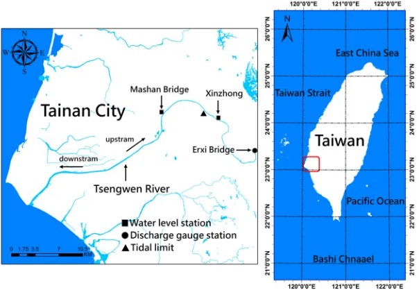
The Tsengwen River is the second largest river in Taiwan and drains into the southern Taiwan

Strait (Figure 1). The drainage basin has an area of 1177 km2_{, which includes part of the}

southwestern rugged foothills and fertile coastal plains. The tide is the primary tidal constituent at

the river mouth and has a mean tidal range below 1 m. Based on the tidal classification [8], the Tsengwen River mouth can be classified as a microtidal estuary [9,10].

Figure 1. Maps of the study area (white, blue, and cyan represent land, ocean, and river, respectively).

Most of the researchers focused on developing an algorithm that interpolated river cross section

measurements to produce a smooth river bathymetry suitable for use in flow modeling. In the present paper, three algorithms including linear interpolation, inverse distance weighting (IDW),

(3)

transverse and longitudinal directions from the originally measured data points. The 2D and 3D

hydrodynamic models were then used to simulate river stages using the original and resampled cross-section data under the low flow and high flow conditions in the Tsengwen River of northern

Taiwan. The simulated results with different river bed cross-sectional data were presented and then sensitivity analyses regarding to the bottom drag coefficient and vertical eddy viscosity were investigated; finally, conclusions were drawn.

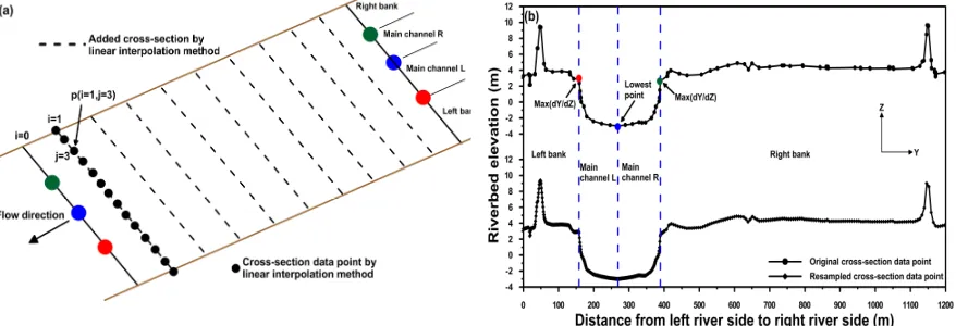
Figure 2. (a) Conceptual diagram of the resampling method and (b) comparison of the original and resampled

cross-sectional data points.

2. Materials and Methods

2.1. Methods for Resampling River Cross-section Data

The 2D/3D numerical simulation of the water stage and river flow requires a large amount of topographic data to build an accurate finite element mesh. The cross-sectional data were measured

in 2012 at every 500-890 m interval that was collected from the Water Resources Agency, Taiwan. To obtain fine cross-section data for grid generation, a resampling the original cross-89 section was

necessary. In the present study, three interpolation approaches (i.e. linear interpolation, IDW, and NN) are adopted to resample the cross-sectional data from the original sample.

2.1.1. Linear interpolation

The linear interpolation algorithm is composed of four steps. The first step is to find the lowest

point and the maximal slope point of the lowest point from each original cross-section for the left and right banks. Each cross section is divided into four parts, including the left bank, main channel L, main channel R, and right bank (shown in Figure 2). The second step is to redistribute the number

of cross-sectional data points based on these four parts and to use linear interpolation in the transverse direction along each original cross section to yield the elevation of each new

cross-sectional data point. The third step is to generate the extra cross sections and data points between each pair of original cross sections in the longitudinal direction using linear interpolation.

Therefore, each part at each cross section has an equal number of points. Finally, linear interpolation is conducted to obtain the elevation between the corresponding parts of each cross section. After

resampling, the new cross-section data set contains the refined cross section with an equal number of the data points.

(4)

part as well as 200 points at the left bank part and right bank part. Figure 2a shows a conceptual

diagram of this resampling method. Figure 2b depicts the resampled cross-sectional data points generated by the linear interpolation method, which satisfactorily maintains the topographic

features of the original sample. After resampling, the maximal distance for each cross section is reduced from 890 m to 80 m. The maximal distance for each data point at the same cross section is reduced from 150 m to 6 m. It should be noted that linear interpolation can avoid the artificial local

maximum and minimum [7].

2.1.2. Inverse Distance Weighting (IDW)

The IDW interpolation is a deterministic, nonlinear interpolation technique. This method uses a weighted average of the attribute values from nearby sample points to estimate the magnitude of

that attribute at non-sampled locations. The weight of any known point is set inversely proportional to its distance from the estimated point [11]. The equation for the IDW interpolation in a

two-dimensional plane is given as:



= =

=

n i i n i m e

d

y

x

p

y

x

P

1 1

1 )

,

(

)

,

(

(1)

where

P

_e

(

x

,

y

)

is the estimated value at (

x

,

y

);

p

_m

(

x

,

y

)

is the measured data point; and

d

_iis

distance from the measured data points to the point which is to be estimated.

2.1.3. Natural Neighbor (NN)

The NN interpolation is a method of spatial interpolation which was developed by Sibson [12]. This method is based on Voronoi tessellation of a discrete set of spatial points and is quite popular in

many fields. The NN interpolation is a weighted moving average technique that uses geometric relationships in order to choose and weight nearby points. The equation for the NN interpolation in a two-dimensional plane is:

)

,

(

)

,

(

1

y

x

p

w

y

x

P

m n i i e



=

(2)

where

w

_i is the weight depended on the area about each of the data points (i.e. Voronoi polygons).

2.2. Three-Dimensional (3D) Hydrodynamic Model

To compare the performance of simulating the river stages using original and resampled river bed cross-section data, a two-dimensional semi-implicit Eulerian-Lagrangian finite element model,

SELFE-2D, was implemented to calculate the river stages in the Tsengwen River. Moreover, the three-dimensional version of SELFE was employed to compare the simulated river stages with the

SELFE-2D modeling results.

SELFE-3D solves the three-dimensional shallow-water equations with the hydrostatic and

(5)

discharge hydrographs upstream are the driving forces in the model. The governing equations of

SELFE-3D can be found in Zhang and Baptista [13].

2.3. Two-Dimensional (2D) Hydrodynamic Model

All variables used in the SELFE-3D model become depth-averaged applied in the SELFE-2D

model, and this model only deals with the barotropic mode. The two-dimensional version of SELFE solves the depth-integrated momentum and continuity equations. The governing equations of

SELFE-2D can be found in Zhang et al. [14] and Zhang et al. [15].

2.4. Model Implementation

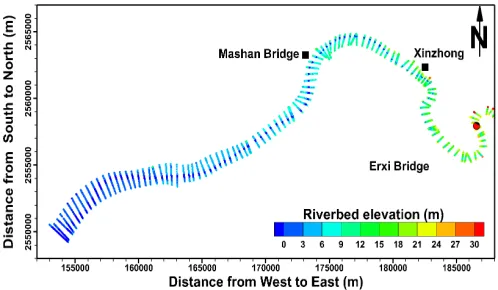
The distribution of the river bed elevation for the original cross-section data is shown in Figure 3. The river bed elevation is low at the downstream reaches, while is high at the upstream and the

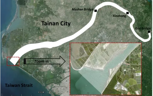
elevation reaches 20 m. Triangle meshes with a resolution of approximately 20 m are deployed from the Tsengwen River mouth to the Erxi Bridge, which is the location of the discharge gauge station. Figure 4 shows the mesh generation in the model domain. The sub-figure of Figure 4 focuses on the

vicinity of the Tsengwen River’s mouth to see the triangle meshes more clearly. The model grid consists of 259,567 elements and 132,136 nodes in the horizontal plane. Once the model meshes are

generated, the different interpolation methods are adopted for interpolating the cross-sectional data to each grid. The river bed elevations that were interpolated from the original cross-section data and

resampled in the cross-section data using different interpolation methods are shown in Figure 5. The resampled river cross-section data produce a similar river topography to the original river

cross-section data in the straight river segments of the Tsengwen River. However, the resampled river cross-section data using the liner interpolation method (Figure 5b) generate better and more reasonable river topography than the original cross-section data (Figure 5a) and the IDW and NN

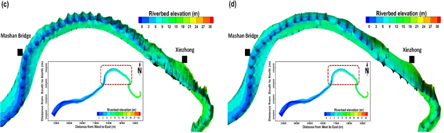
methods (Figures 5c and 5d) in the meandering river segment of the Tsengwen River. The 3D views of the meandering segment of the Tsengwen River are illustrated in Figure 6. The rugged river bed

can be found in Figures 6a, 6c, and 6d. However, the river bed shows a smoothing pattern at the same river segment (Figure 6b). A minimum depth of 0.01 m was indicated as a criterion for the

wetting and drying simulation. A time step of 10 seconds was used in the simulation without any signs of numerical instability.

(6)

Figure 4. High resolution unstructured grids in the Tsengwen River for hydrodynamic modeling.

Figure 5. River bed elevation used for hydrodynamic modeling; (a) original cross-sectional data and resampled

(7)

Figure 6. A 3D view of the river bed elevation of the hydrodynamic model using (a) the original data and

resampled data according to (b) the linear interpolation method, (c) the IDW method, and (d) the NN method.

The red dashed box in the sub-figure represents the location of the 3D view river segment in the Tsengwen

River.

2.5. Assessment of the Model Performance

To assess the model performance using different river cross-sectional data for simulating the

river stages, three criteria are adopted: the mean absolute error (MAE), the root mean square error (RMSE), and the percent bias (PBIAS). The equations for these three criteria are as follows:

1

N s m i i i

MAE

N

=

η η

=



−

(3)

(

)

2

1

N s m i i i

RMSE

N

₌

η η

=



−

(4)

1 1

100

n s m i i i n m i i

PBIAS

η η

η

= =

−

=



×



(5)

where

η

_is is simulated river stage and

η

_im is measured river stage.

3. Results

3.1. Simulation of the River Stage Using Different Cross-Section Data

Two data sets of hourly discharge hydrographs were extracted and imposed on the upstream boundary condition at the Erxi Bridge (a distance of 50 km from the Tsengwen River’s mouth). One

period is from June 2 to June 6, 2012 (i.e., low flow condition), and the other one is from June 11 to June 16, 2012 (i.e., high flow condition). The tidal elevations at the Tsenweng River’s mouth were

calculated using the regional tidal prediction model of the South China Sea [16], which served as the downstream boundary condition. The measured river stage data were used to evaluate the performance on the simulation of the river stage using different river cross-section data. The initial

conditions of the water surface are set equal to the riverbed elevations. All meteorological forces are not considered in the model.

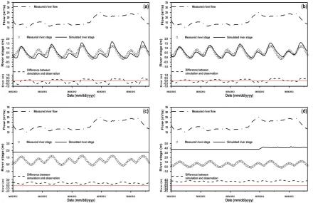
Figure 7 shows the model-data comparison of the river stages at the Mashan Bridge under low flow conditions using the 2D model with the original (Figure 7a) and resampled cross-section data

(8)

river stage at the middle panel, and the error between simulated and observed river stages at the

lower panel. Because the Mashan Bridge is located at the tidal river reach of the Tsengwen River, Figure 7 reflects the river stage variations affected by flood and ebb tides. The simulated river stage

using the original cross-section daurea (Fig. 7a) shows smaller amplitudes than the resampled cross-section data using the linear interpolation method (Figure 7b). This result means that the tidal wave has slight difficulty reaching upstream if the original cross-section data are used for model

simulation. The simulated river stages using the resampled cross-section data according to the IDW and NN interpolation methods show straight line with time (Figures 7c and 7d). It means that the

simulated river stage is not affected by tide at the Mashan Bridge. The simulated river stages are quite different with the measured results.

Figure 7. A comparison of the simulated and observed river stages at the Mashan Bridge under the low flow

condition using the 2D model with the (a) original cross-section data and resampled cross-section data

according to (b) the linear interpolation method, (c) the IDW method, and (d) the NN method.

The blocked phenomenon of the river channel is shown at the Xinzhong station using the

original cross-section data (Figure 8a). Figure 8a shows that the riverbed cannot become wet at the Xinzhong station until 1:00 on June 5, 2012, and Figure 8b reveals the consistency between the simulated and observed river stages using the resampled cross-section data (i.e. linear interpolation

method). The simulated river stages extremely overestimate the measured river stage using the resampled cross-section data according to the IDW and NN methods (Figures 8c and 8d). Figure 9

presents the distribution of the simulated river stages in the Tsengwen River using the original and different resampled cross-section data. The river stages show discontinuity between the Mashan

Bridge and the Xinzhong station, which is a meandering river reach of the Tsengwen River (Figures 9a, 9c, and 9d). The figures also show that the river stages are abnormally high upstream of the

(9)

Figure 8. A comparison of the simulated and observed river stages at the Xinzhong station under low flow

conditions using the 2D model with the (a) original cross-section data and resampled cross-section data

Figure 9. Simulated river stage distribution at 618 1:00 on June 5, 2012, under the low flow condition using the

2D model with the (a) original cross-section data and resampled cross-section data according to (b) the linear

interpolation method, (c) the IDW method, and (d) the NN method.

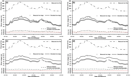
Figures 10 and 11 illustrate the model-data comparison of river stages, respectively, at the

(10)

cross-section data (i.e. linear interpolation method) show good agreement with the measured river

stages at both the Mashan Bridge and Xinzhong stations but overestimate when the river flows

exceed approximately 1,500 m3_{/s. Although the simulated river stages using the original}

cross-section data show an acceptable result at the Mashan Bridge (Figure 10a), the simulated river stage cannot be lowered, even if there has been a decrease in the river flows (Figure 11a). This result means that the riverbed elevations interpolated by the original cross-section data are higher than the

actual ones. The simulated river stages using the resampled cross-section data based on the IDW and NN methods extremely overestimate the measured river stages at both the Mashan Bridge and

Xinzhong stations shown in Figures 10c, 10d, 11c, and 11d.

The river stage distribution at 12:00 on June 12, 2012, using the original and different resampled

cross-section data is shown in Figure 12. Figure 12a and Figure 12b display similar simulated results, but the river stages around Xinzhong station are higher using the original cross-section data than

those using resampled cross-section data based on the linear interpolation. Comparing to Figures 12b, 12c, and 12d, the simulated river stages between the Mashan Bridge and Xinzhong station using resample cross-section data according to the IDW and NN methods are extremely higher than those

using the linear interpolation method. Based on the modeling results above, the bottom drag coefficients are set to be 0.002.

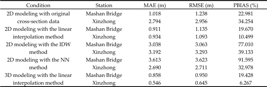
Statistical errors between the simulated and measured river stages for different river bed cross-section data using the 2D model under low flow and high flow conditions are presented in

Table 1 and Table 2, respectively. The results indicate that the MAE, RMSE, and PBIAS values with the resampled cross-section data using the linear interpolation method are lower than those with the

original and resample cross-section data using the IDW and NN methods at the Mashan Bridge and Xinzhong station under both the low and high flow conditions.

Figure 10. A comparison of the simulated and observed river stages at the Mashan Bridge under the high flow

condition using the 2D model with the (a) original cross-section data and resampled cross-section data

(11)

Figure 11. A comparison of the simulated and observed river stages at the Xinzhong station under high flow

conditions using the 2D model with the (a) original cross-section data and resampled cross-section data

Figure 12. Simulated river stage distributions at 12:00 on June 12, 2012, under the high flow condition using the

2D model with the (a) original cross-section data and resampled cross-section data according to (b) the linear

(12)

Table 1. Statistical error between the simulated and measured river stages under the low flow condition.

Condition Station MAE (m) RMSE (m) PBIAS (%)

2D modeling with original cross-section data

Mashan Bridge 0.304 0.346 -17.13

Xinzhong 3.627 3.750 87.090 2D modeling with the linear

interpolation method

Mashan Bridge 0.203 0.232 1.229

Xinzhong 0.133 0.151 -3.285 2D modeling with the IDW

method

Mashan Bridge 1.190 1.250 214.385

Xinzhong 4.220 4.367 104.055

2D modeling with the NN method

Mashan Bridge 3.328 3.353 599.405

Mashan Bridge 0.216 0.253 3.390

Xinzhong 0.096 0.105 -1.404

Table 2. Statistical error between the simulated and measured river stages under the high flow condition.

Condition Station MAE (m) RMSE (m) PBIAS (%)

2D modeling with original cross-section data

Mashan Bridge 1.018 1.238 22.981

Mashan Bridge 0.911 1.135 19.670

Xinzhong 0.934 1.093 10.499 2D modeling with the IDW

method

Mashan Bridge 3.038 3.063 77.010

Xinzhong 3.192 3.293 39.133 2D modeling with the NN

method

Mashan Bridge 3.613 3.623 91.595

Mashan Bridge 0.858 0.950 19.428

Xinzhong 0.546 0.645 6.267

3.2. Comparison of the Simulated River Stage Using the 2D and 3D Models

To compare the performance between the 2D and 3D models on the simulation of the river stage, the samplings with the 2D and 3D models were conducted with the same grids, initial

conditions, and boundary conditions using the resampled river bed cross-section data based on the linear interpolation method which is the best performance using 2D model shown in Tables 1 and 2. In the 2D and 3D models, the same bottom drag coefficients are used and set to be 0.002. The vertical

eddy viscosity in 3D model is set to be 1.5x10-4_m2_/s.

Figure 13 compares the simulated and measure river stages using the 2D and 3D models at the

Mashan Bridge (Figure 13a) and the Xinzhong station (Figure 13b) under the low flow condition. The simulated results of the 2D model and the 3D model are identical at the Mashan Bridge, but the

simulated river stage of the 3D model is slightly higher than that of the 2D model at the Xinzhong station (Figure 13b). Figure 14 compares the simulated and measured river stages of the 2D and 3D

models under the high flow condition. The 3D modeling results indicate that the simulated river stages are a closer match to the measured river stages compared to the 2D modeling results at both the Mashan Bridge (Figure 14a) and Xinzhong station (Figure 14b). Figure 15 presents the

distributions of simulated river stage using the 3D model with the resampled cross-section data under the low flow (Figure 15a) and high flow (Figure 15b) conditions at 1:00 on June 5, 2012. The

figure shows that the distributions of the simulated river stage are very reasonable.

To compare the performance of the 2D and 3D models using the resampled cross-section data

(13)

2D model is better than that of the 3D model with the low condition at the Xinzhong station, whereas

the performance of the 2D model is inferior to that of the 3D model at the Mashan Bridge (Table 1). For the high flow condition, the performance 283 of the 3D model is better than that of the 2D model

at both the Mashan Bridge and Xinzhong station (Table 2).

Figure 13. Comparison of the simulated river stages using the 2D and 3D models with the resampled

cross-section data under the low flow condition at the (a) Mashan Bridge and (b) Xinzhong station.

Figure 14. Comparison of the simulated river stages using the 2D and 3D models with the resampled

(14)

Figure 15. Simulated river stage distribution using the 3D model with the resampled cross-section data (a) at

1:00 on June 5, 2012, (low flow condition) and (b) at 12:00 on June 12, 2012 (high flow condition).

3.3. Model Sensitivity

Prandle [17] reported that for tidal propagation in depths greater than 50 m, bottom friction is of secondary importance and 2D models are adequate to calculate integrated transport. Conversely,

the increasing importance of both bottom friction and vertical eddy viscosity in shallow water indicated the requirement for 3D models. Sensitivity analysis is a power methodology that can be

used to improve the understanding of how the bottom drag coefficient and the vertical eddy viscosity affects the river stages in the Tsengwen River. The sensitivity analysis was conducted by

running the 2D and 3D models with all the conditions described in previous section, except for the bottom drag coefficient and the vertical eddy viscosity. The original base depended on the simulation of low flow and high flow conditions.

To investigate the effects of bottom drag coefficient on the river stage, the 2D and 3D models using the resampled cross-section data based on the linear interpolation method were run using two

alternative cases. One method calculated the value of bottom drag coefficient 50% higher than the original base run, and the other method calculated the value of bottom drag coefficient 50% lower

than the original case run. Table 3 and Table 4 show the modeling results of sensitivity runs under low flow and high flow conditions, respectively. The maximum rate of river stage was used to

(15)

base base sens

MR

η

−

=

(6)

where

η

base is the river stage for the base run and

η

sens is the river stage for the sensitivity run.

Positive and negative values of maximum rate represent the increase and decrease in river stage, respectively.

The maximum rates for increasing bottom drag coefficient are 0.615% and 0.08%, respectively, at the Mashan Bridge and Xinzhong station using 2D model under low flow condition, whereas the

maximum rates for decreasing bottom drag coefficient were -1.037% and -0.069% (Table 3). The maximum rates for increasing bottom drag coefficient are 2.612% and 5.96%, respectively, at the

Mashan Bridge and Xinzhong station using 2D model under high flow condition, whereas the maximum rates for decreasing bottom drag coefficient are -0.267% and -4.217% (Table 4). The

results of model sensitivity using 3D under low and high flow conditions are also displayed in Tables 3 and 4. We found that the increasing bottom drag coefficient resulted in the increasing river stage. It is the reason that the increasing the bottom drag coefficient can increase the total resistance

and lead to decrease the velocity which results in the increase of river stage [18]. The modeling results indicate that the bottom drag coefficient has a minor impact on river stage using 2D and 3D

models.

Because the vertical eddy viscosity was included in 3D model only, the model sensitivity runs

were conducted using 3D hydrodynamic model. The maximum rates for increasing vertical eddy viscosity are 0.943% and 0.506%, respectively, at the Mashan Bridge and Xinzhong station under

high flow condition, whereas the maximum rates for decreasing vertical eddy viscosity are -0.945% and -0.508% (Table 4). The maximum rates for increasing and decreasing vertical eddy viscosities

under low flow condition (Table 3) are lower than those under high flow condition (Table 4). Miller and Cluer [19] examined the water level response to different eddy viscosity. They also found that the increasing eddy viscosity raised the water level. However, in the current study, the modeling

results reveal that the vertical eddy viscosity is insensitive to river stage.

Table 3. The influence of model sensitivity runs on river stage under low flow condition.

Condition Station Maximum rate of river stage (%)

2D modeling with increasing 50% BDC

Mashan Bridge 0.615

Xinzhong 0.081

2D modeling with decreasing 50% BDC

Mashan Bridge -1.037

Xinzhong -0.069

Mashan Bridge 0.208

Xinzhong 0.002

3D modeling with decreasing 50% BDC

Xinzhong -0.005

3D modeling with increasing 50% VEV

Mashan Bridge 0.001

Xinzhong 0.009

3D modeling with decreasing 50% VEV

Xinzhong -0.007

(16)

Table 4. The influence of model sensitivity runs on river stage under high flow condition.

Condition Station Maximum rate of river stage (%)

Mashan Bridge 2.612

Xinzhong 5.960 2D modeling with decreasing

50% BDC

Xinzhong -4.217 3D modeling with increasing

50% BDC

Mashan Bridge 1.309

50% BDC

Xinzhong -0.0001 3D modeling with increasing

50% VEV

Mashan Bridge 0.943

50% VEV

Xinzhong -0.508 Note: BDC: Bottom drag coefficient; VEV: Vertical eddy viscosity

4. Discussion

A large amount of accurate measurements of the river cross-section data is indispensable for simulating river stages using 2D and 3D models. However, the measured river cross-section data are

usually sparse in spatial resolution. If the original (sparse) river cross-section data are employed, a rough and uneven river bed is created. This phenomenon is especially obvious in a meandering river

segment (shown in Figures 5a and 6a) because the distance between two measured river cross sections is too far to make a correct interpolation. Because of the rugged river bed elevations, the

water is blocked in the channel and consequently delays the arrival time of water from upstream to downstream, resulting in the an extremely high river stage at upstream reaches (shown in Fig. 9a). A

similar phenomenon has been reported by Cook and Merwade [20]. They demonstrated that different amounts of the river cross-section data produced different amounts of coverage of the water surface.

In Figure 14, the simulated river stage using the 2D model is higher than that using the 2D model under the high flow condition when the river flow exceeds 1,500 m3_{/s. If the Coriolis force,}

tidal effect, atmospheric pressure at the free surface, and wind shear stress are neglected, and a steady state is assumed, the momentum equation can be expressed as:

gH

x

bx 0

ρ

τ

η

₌

₋

∂

(7)

where H =

η

+h ;

h

is the bathymetric depth;

η

is the free-surface elevation; g is the e

acceleration due to gravity;

ρ

₀ is the density of water; and

τ

_bx is the bottom shear stress in x

direction.

Eq. (7) shows that

η

is affected by the bottom shear stress in the models. The equation

indicates that

η

increases with increasing bottom shear stress. The velocity gradient (

z

u

∂

_{) is}

positive based on the bottom shear stress (

τ

). One layer is used to calculate

z

u

∂

_{in the 2D model,}

(17)

using the 3D model, resulting in a worse performance when the 2D model is used (Figure 14). A

similar theory used to discuss the wind stress tide can be found in Dean and Dalrymple [21].

5. Conclusions

This study applied three algorithms including linear interpolation, IDW, and NN to refine river

cross-section data based on original data. The resampled cross-section data based on the linear interpolation satisfactorily maintains the topographic and morphological features of the river

channel, especially at the meandering river reach. The river channel constructed by the resampled cross-section data based on the linear interpolation is more flat and smooth than the model created

by the original cross-section data, IDW, and NN interpolation. The 2D high-resolution unstructured-grid hydrodynamic model was adopted to assess the performance between the

simulated and measured river stages with the original and resampled cross-section data under low flow and high flow conditions. The results indicate that the simulated river stages are improved significantly to match the measured river stages using the resampled cross-section data based on the

linear interpolation at the tidal river and non-tidal river stations.

Furthermore, the performance between the simulated and measured river stages using the 2D

and 3D models incorporated with the resampled cross-section data based on the linear interpolation were evaluated. The results show that the simulated river stages using the 2D and 3D models

reproduce the measured river stages at both the tidal and non-tidal river stations under the low flow condition. However, the simulated river stages using the 2D model overestimate the measured river

stages at both the tidal and non-tidal river stations under the high flow condition. The 2D model is appropriate for real-time river stage prediction for flash flood warning because it requires less computational time, but the 3D model provides a more accurate simulation of the river stage. The

model sensitivity was conducted by increasing and decreasing the bottom drag coefficient and vertical eddy viscosity. The modeling results indicate the bottom drag coefficient has a minor impact

on river stage and the vertical eddy viscosity is insensitive to river stage.

The algorithm developed for riverbed interpolation is very useful in cases where the river

bathymetry is frequently modified by hydrological events, for example, in restored river sections. This is because periodic flow modeling is required to assess how river morphology affects ecological

aspects [22]. Further study will be needed to define more specifically the optimal cross-section spacing in relation to the grid resolution.

Acknowledgments: This project was funded by the Ministry of Science and Technology (MOST), Taiwan, grant No. 104-2625-M-239-002. The authors would like to thank the Taiwan Water Resources Agency for providing the measured data.

Author Contributions: Wen-Cheng Liu supervised the progress of the MOST project and served as a general editor. Wei-Bo Chen performed the data collection, model establishment, and model simulations and discussed the results with Wen-Cheng Liu. All authors read and approved the final manuscript.

Conflicts of Interest: The authors declare no conflict of interest.

References

1. Chen, W.B.; Liu, W.C.; Wu, C.Y. Coupling of a one-dimensional river routing model and a three-dimensional ocean model to predict overbank flows in a complex river-ocean system. Appl. Math. Model.2013, 37, 6163-6176.

(18)

3. Merwade, V.M.; Cook, A.; Coonrod, J. GIS techniques for creating river terrain models for hydrodynamic modeling and flood inundation mapping. Environ. Model. Softw. 2008, 23, 1300-1311.

4. Horritt, M.S.; Bates, P.D.; Mattinson, M.J. Effects of mesh resolution and topographic representation in 2D finite volume models of shallow water fluvial flow. J. Hydrol.2006, 329, 306-314.

5. Tomczak, M. Spatial interpolation and it uncertainty using automated anisotropic inverse distance weighting (IDW)-cross-validation/Jackknife approach. J. Geogr. Inform. Decis. Anal.1998, 2, 18-30.

6. Schappi, B.; Perona, P.; Schneider, P.; Burlando, P. Integrating river cross section measurements with digital terrain models for improved flow modeling applications. Comput. Geosci.2010, 36, 707-716.

7. Caviedes-Voullieme, D.; Morales-Hernandez, M.; Lopez-Marijuan, I.; García-Navarro, P. Reconstruction of 2D river beds by appropriate interpolation of 1D cross-sectional information for flood simulation. Environ. Model. Softw.2014, 61, 206-228.

8. Dyer, K.R. Estuaries: A physical introduction. New York, Wiley, 1997.

9. Chen, W.B.; Liu, W.C. Modeling flood inundation induced by river flow and storm surge over a river basin. Water 2014, 6, 3182-3199.

10. Wei, H.P.; Yeh, K.C.; Liou, J.J.; Chen, Y.M.; Cheng, C.T. Estimating the risk of river flow under climate change in the Tsengwen River Basin. Water2016, 8, 81.

11. Isaaks, E.H.; Srivastava, R.M. Applied geostatistics. Oxford University Press, New York, 1989; 257-258. 12. Sibson, R. A brief description of natural neighbor interpolation. In: Interpreting Multivariate Data. Barnett, V.

(Editor), John Wiley and Sons, New York, 1981; 21, 21-36.

13. Zhang, Y.; Baptisa, A.M. SELFE: a semi-implicit Eulerian-Lagrangian finite-element model for cross-scale ocean circulation. Ocean Model.2008, 21, 71-96.

14. Zhang, Y.J.; Witter, R.C.; Priest, G.R. Tsunami-tide interaction in 1964 Prince William Sound tsunami. Ocean Model.2011, 40, 246-259.

15. Zhang, Y.; Ye, F.; Stanev, E.V.; Grashorn, S. Seamless cross-scale modeling with SCHISM. Ocean Model. 2016, 102, 64-81.

16. Zu, T.; Gana, J.; Erofeevac, S.Y. Numerical study of the tide 456 and tidal dynamics in the South China Sea. Deep Sea Res. Part I2008, 55, 137-154.

17. Prandle, D. The influence of bed friction and vertical eddy viscosity on tidal propagation. Cont. Shelf Res. 1997, 17, 1367-1374.

18. Kim, T.B.; Choi, S. Depth-averaged modeling of vegetated open-channel flows using finite element method. Proceedings of 16th IAHR-APD Congress and 3rd Symposium of IAHR-ISHS, Chapter in Advances in Water Resources and Hydraulic Engineering, Spring 426 Berlin Heidelberg, 2008; Vol. II, 411-416.

19. Miller, A.J.; Cluer, B.L. Modeling considerations for simulation of flow in bedrock channels. In: Rivers over Rock: Fluvial Processes in Bedrock Channels, Tinkler, K.J., Wohl, B.L. (Eds.), American Geophysical Union, Geophysical Monograph Series, 2013; Vol. 107, 61-104.

20. Cook, A.; Merwade, V. Effect of topographic data, geometric configuration and modeling approach on flood inundation mapping. J. Hydrol.2009, 377, 131-142.

21. Dean, R.G.; Dalrymple, R.A. Coastal processes with engineering applications. Cambridge University Press, UK, 2004.

22. Wohl, E.; Angermeier, P.L.; Bledsoe, B.; Kondolf, G.M.; MacDonnell, L.; Merritt, D.M.; Palmer, M.A.; Poff, N.L.; Tarboton, D. River restoration. Water Resour. Res.2005, 41, W10301-1-W10301-12.