A
Comparison Between
MFA
and
GNC
Griff
L.
Bilbro
Center for Communications and Signal Processing
Department Electrical and Computer Engineering
North Carolina State University
A Comparison between MFA and GNC
Griff L. Bilbro
September 26, 1990
1
Introduction
We will show that Mean Field Annealing (MFA) provides a unified approach to several difficult optimization problems. All the resulting MFA algorithms resemble the Graduated Nonconvexity Algorithm (GNC) developed by Blake and Zisserman(4] to solve certain image processing problems. MFA is based on Simulated Annealing (SA) and derives its power and generality from that popular optimization procedure. MFA differs from SA by analytically ap-proximating the relevant Gibbs distribution rather than stochastically
simu-lating it. ,
Simulated Annealing is slow but is otherwise simple, general, easy to apply to new problems, and remarkably successful even when theoretical conditions for convergence are not met(10]. SA works by gradually cooling an on-going stochastic simulation of a Gibbs distribution. Mean field theory provides a deterministic approximation to a Gibbs distribution which also can be cooled in the same way to produce a Mean Field Annealing (MFA) algorithm. Many SA algorithms can be converted to analogous MFA al-gorithms that run in 1/50 the time required by the SA version[9, 1, 8, 2]. However because it is an approximation, MFA does not inherit any guarantee of convergence even when the analogous SA does converge.
The mean field is usually restricted to Ising-like systems described by an energy function (or Hamiltonian) involving binary variables 8
==
{Si}~~fH[s]
== -
L
hisi -L
Vij Si 8j,ij
1
but recently we have extended MFA to a wider class of problems. This extension depends on Peierls' inequality F ::; W which bounds the exact free energy at temperature T of a system of 8 described by Equation 1
F
==
-TInL
exp(-HIT), {a}by the Weiss free energy W
W ==
F
o+
(H - Ho).(2)
(3)
Here Ho is an arbitrary function of s. The average is with respect to the
density Zolexp(-HolT) normalized over all possible configurations of the
s by the factor
z;
==
L
exp(-HolT)(4)
which is also used to define Fo
==
-TInZOeThe free energy F function characterizes the equilibrium of the system described by Equation 1 at temperature T. The utility of the bound F ::;
W is that it -remains valid even if Ho depends on adjustable parameters
in addition to S. It can be shown[3] that equality obtains if and only if
Ho
==
H. In this mean field sense, adjusting Hoto minimize W adjusts Hotomost closely resemble H. Even Peierls inequality was previously restricted to Ising-like problems, but we have recently shown how to choose Hoto treat continuous variables as well[8, 2]. Peierls' inequality was originally derived in the context of statistical mechanics, but we have recently constructed an information-theoretic derivation [3] .
MFA converts an optimization problem into the limiting member of a
family of optimization problems. Instead of directly varying H, MFA varies a certain weighted average of H. The width of averaging kernel depends on a scalar called the temperature T. For small T the kernel approaches a Dirac delta function and in the limit the original problem is recovered. For large T fine structure of the original problem is averaged away and in this limit the objective becomes convex even if the original objective was not. MFA works when the large-T optimum approaches the best (or at least a good) low-T optimum as T is reduced.
to the weak membrane to obtain an algorithm that is qualitatively identi-cal to GNC for the same problem[6]. In this report we will show that MFA generally produces "GNC-like" algorithms for several optimization problems.
2
A binary problem
The H of Equation 1 is useful for graph bisection if Vij is the adjacency matrix, hi reflects some externally specified preference for assigning node i
to a particular partition, and the value of s, determines the assignment of node i[l, 5]. A slightly more complicated form of H has been used to restore binary images[3]. Here consider the simplest one-dimensional case where
hi
==
h,Vi and all v vanish except Vij==
v,'tIj==
i+
1 so thati=N i=N H
==
-hL
Si - vL
Sisi+1i=1 i=1
(5)
with the S connected in a ring 8N+1
==
81' For concreteness we take s, E{-1, +1}.1
If 0
<
h<
v then a descent algorithm cannot reliably find the minimum of H unless its moveset includes flips of at least 2v,j h adjacent variables. To see this, consider global minimum. configuration Si==
1, 'Vi with energyH(O, N)
==
(-h - v)N. Now the configuration Si==
-1,Vi with higher energy H( N,0) == (h - v)N is a local minimum since flipping k consecutivevariables to 1 raises the energy to H(N - k, k)
==
H(N,O) - 2kh+
4v>
H(N,O)
for k<
2v/h. Flipping non-consecutive variables is higher still. There is a "barrier" between the "all-down state" and the global minimum "all-up state". Evidently a successful descent algorithm requires ingenuity to construct its moveset. MFA provides an alternative that requires no such ingenuity.A mean field approximation of the associated Gibbs density is obtained by taking Ho
== -
2:i
XiSi with adjustable mean field parameters x==
{xi}~~f·The sum over configurations becomes
2:3
==
2:31
=±12:3
2= ± 1 · · ·2:3N=±1 so that Zo==
ni
2 coshXi/T, from which Fo==
-T2:
In2 cosh xi/To The average1Any other kind of random binary variable in a Hamiltonian can be algebraically
trans-formed to the range {-1,+1},although special consideration is required if a factor of
sl
occurs anywhere.value of (!Ji) under Ho is related to Xi by the function m
(6)
which tends toward the algebraic sign of Xi for small enough T so that the original binary character of the problem is recovered from MFA at T
==
O. Now (Ho)= -Li
Xim(Xi) and(7)
Combining these we obtain a bound on the free energy F ::; W
which can be minimized with respect to the mean field x. The resulting self-consistency condition on X
(9)
can be converted to an equivalent condition for the expectations rn;
==
m(Xi)h (h
+
V'mi-l+
vmi+1 ) )m, = tan T · (10)
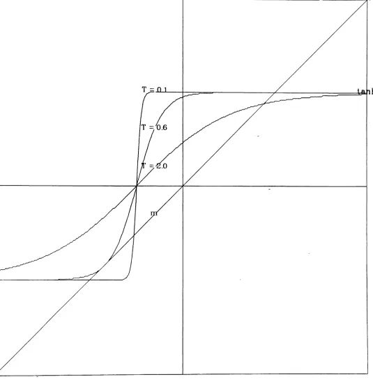
The minimum of W tells us about the thermal equilibrium at T of a system described by H, but to find the minimum ofH we must in general anneal. For our shift invariant choice of h and v, the low W states have shift invariant
tn;
==
m,Vi also. Equation 10 becomes m==
tanh((h+
2vm)IT) which isgraphically solved in Figure 1 for h
==
v==
1 at several values of T. Figure 1 shows that Equation 10 has one solution for high T but three solutions below a certain "critical" T. It can be shown that the middle solution is a maximum of Wand the two extreme solutions are minima. Here the rightmost solution determines the global minimum as T falls. On way to describe this is that MFA varies the non-convexity of the optimization problem as a function of5
Figure 1: Self consistency Equation 10. Graphical solution for m
=
tanh((h+
2vm)/T).
The straight line is y =x.
The curves are y =tanh((h+2vx)/T).
Intersections between the straight lines and curves indicate extrema of W. At high
T
there is only one solution. At lowT,
the problem becomes3
A real-valued problem
The objective or Hamiltonian
H[u]
==
1/2 L:(Ui - di)2 -
AL:
6(Ui - Ui+1)i i
(11)
is minimized by a piecewise constant approximation to d, i.
e.,
when real variables u.; can be chosen to resemble data di and to frequently coincide with neighbors Ui±l. For this problem the simplest useful choice is Ho==
L:i
1/2(ui - lti)2 with real means Iti. The average in Peierls' inequality is weighted by the Gaussian density Zol exp(-Ho/T) now extends over all real configurations. Zo involvesJ:
dUlJ:
dU2 · . ·J:
dUN but it factors so that the normalization is Zo==
TIi
J21rT. The logarithm of a product is a sum of logarithms so that Fo==
-TL:i
InJ2-rrT. The average Ho is a sum of second moments (Ho) ==L:i
T/2
==
NT/2.
For this Ho,both Foand (Ho) areindependent of m. All the m dependence appears in (H) which is the sum of a data term
L:i
1/2((
Ui - di)2)
==
NT/2
and an interaction that involvesthe average of a Dirac delta (h(ti; - Uu+i))
J
dUidui+l 2 221rT exp( -(u; - /Li) - (Ui+l - /Li+l) .
)6(
u, - Ui+l)which can be integrated once with the' Dirac delta
and then evaluated with a table of integrals to obtain
Combining these results
[(It. - d·)2 A ((It.
-II.'
)2)]
ltV
==
constant+
L
1 1 exp _ 1 ,1+1 )i 2
v;rr
4T(12)
(13)
(14)
(15)
Gaussian tends to a Dirac delta as T vanishes. Figure 2 should be compared with Figure 3 where the non-convexity of the clipped parabola is also reduced by increasing T. In both cases MFA prescribes that the high-T solution be followed as T is gradually reduced. MFA replaces a non-convex problem with a family of problems of graduated non-convexity.
Two-dimensional versions of this formulation has been used to remove noise from corrupted observations of real-valued images known to be piecewise-constant[8]. MFA has been used to identify the most effective form for the delta function interaction in two dimensions[7]. Piecewise-linear restorations are similarly obtained by replacing the first difference in the argument of the delta function by the appropriate second difference[2].
4
A mixed problem
A one-dimensional version of Blake and Zisserman's weak membrane energy function[4] is (the weak string function)
i=N
H[u,l]
=
2:
[(Ui -dd
2+
,X2(Ui - Ui+l)2(1- ld
+
ali] , (16)i=1
for binary line field I
=
{Ii}~~f and Ii E {O,I}, real intensities u = {ui}~~fand u.; E (-00,00) and data d = {di}~~f. For simplicity take UN+1
==
U1' The parameter A is an elastic constant and Q controls when the elasticity saturates,It is possible to treat both u and I as random fields and apply mean field theory to both, but Blake and Zisserman are concerned with non-convexities due to discrete I, so restrict Ho to the energy of I given the mean field x
H
o= -
2:
XiIi.(17)
Working toward Peierls' inequality, we will compute averages with the density
Z(;l exp(-HolT). The normalization involves the sum over all configurations
~ _ '""" _ .• '~, -0t : But the sum of products factors into a product
LJlt-O,1 LJI2-0,1 L..JN - , .
of sums to give Zo
=
ni(1+
exp(xi/T)).
From this Fo=
-TEiln (1+
exp(xdT)).
The expectation of the random variable l; are related to themean field parameter Xi as (Ii) == U(Xi) where
o
+
e:r;/T 1 (18)0"(
Xi)
=
1+
e:r;/T=
1+
e-:r;fT'T 0.01
8
T
8
In terms of a
and
(Ho)
= -
L
Xi U( Xi). i(19)
i=N
(H) =
L
[(Ui - dd 2+
,\2(Ui -ui+d
2(1 - u(xd)+
Q:U(Xi)] · (20)i=l
Combining these, the Weiss free energy W is
L
[-TIn(l+
ellli l T)
+
(Ui - dd 2+
,\2(Ui - ui+d2(1 - u(xd)+
Q:U(Xi)+
XiU(Xi)] . i(21)
The optimal value of x is determined by solving the system
(22)
which occurs when
(23)
which depends on the u field. Substituting Equation 23 into Equation 21 yields
~
[
2
(
;\2(Ui - Ui+l)2 -a)
2(
)2]
mjnW(u,x)
=
L.:
(Ui - dd - TIn 1+
exp T+,\
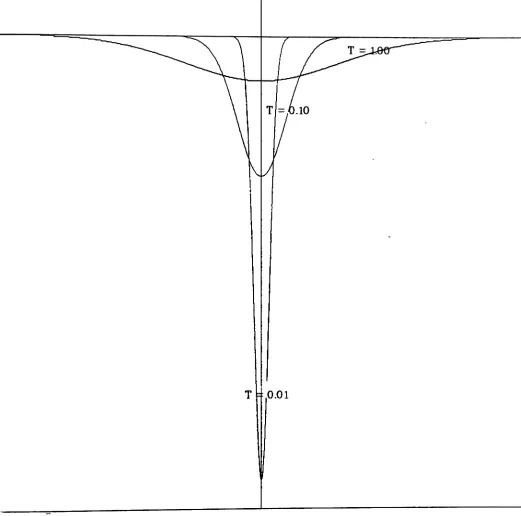
u; - Ui+l ,(24) which is then to be minimized with respect to u (here by simple gradient descent) to determine the mean field approximation to thermal equilibrium at T. MFA prescribes that the minimum min.j; W(u, x)
=
min., min, W(u, x)be annealed to find the minimum of H,but this is essentially G NC as was first reported by Geiger and Girosi who called the last two terms of Equation 24 the "effective potential". In Figure 3, this effective potential is plotted against
u, - Ui+l for several values ofT. Note that for T ::; .2 this plot is qualitatively
10
(
~2(U' u· )2
ex)
2(
2
Figure 3: A plot of -TIn 1
+
exp . ,-.jy. -+
A u.; -uHd
the lasttwo terms of Equation 23 against the difference u.; - Ui+l for several values
The mean field approximation itself does not explain the superiority of MFA piecewise-constant restorations over GNC weak-membrane restorations. MFA applied to the weak membrane approximates Blake and Zissermans GNC algorithm. MFA applied to an objective with a delta function interac-tion produces our previous MFA algorithms for piecewise constant restora-tion. We conclude that MFA produces better piecewise constant restorations than GNC because a delta function interaction is a better model of piecewise constant surfaces than is the weak membrane. The weak membrane of GNC models the scene with a piecewise smooth objective which is less appropriate for scenes that are really piecewise constant.
References
[1] G. L. Bilbro, T. K. Miller, W. E. Snyder and D. E. Van den Bout, M. W. White, and R. C. Mann. Optimization by the Mean Field Approxima-tion. In Advances in Neural Network Information Processing Systems 1,
pages 91-98. Morgan-Kauffman, San Mateo, 1989. Reprinted from 1988 NIPS, Denver, CO.
[2] G. L. Bilbro and W. E. Snyder. Mean field annealing: An application to image noise removal. Journal ~fNeural Network Computing, 1990.
[3] G. L. Bilbro, W. E. Snyder, and R. C. Mann. The mean field minimizes relative entropy. Journal of the Optical Society of America A, 1991. To appear.
[4] A. Blake and A. Zisserman. Visual Reconstruction. The MIT Press, Cambridge, Mass., 1987.
[5] D. E. Van den Bout and T. K. Miller. Graph partitioning using annealed neural networks. IEEE Trans. Neural Networks, 1(2):192-203, 1990.
[6] D. Geiger and F. Gitosi. Parallel and deterrninist.ic algorithms for rnrfs: surface reconstructin and integration. Technical Report A. I. Memo No. 1114, Massachusetts Institute of Technology, 1989.
[7] H. P. Hiriyannaiah. Signal reconstruction using mean field annealing.
[8] H. P. Hiriyannaiah, G. L. Bilbro, W. E. Snyder, and R. C. Mann. Restoration of piecewise constant images via mean field annealing. Jour-nal of the Optical Society of America A, pages 1901-1912, December 1989.
[9]
C.M.
Soukoulis,K.
Levin, and G.S.
Grest. Irreversibility and metasta-bility in spin-glasses. i ising model. Phys. Rev. B, 28(3):1495-1509,August 1983.
[10] P. J. M. van Laarhoven and E. H. L. Aarts. Simulated Annealing: Theory and Applications. D. Reidel, Norwell, Mass, 1988.