Performance limits of channel parameter estimation for joint communication and positioning

R E S E A R C H

Open Access

Performance limits of channel parameter

estimation for joint communication and

positioning

Kathrin Schmeink

, Rebecca Adam and Peter A Hoeher

Abstract

Recently, a system concept for joint communication and positioning has been proposed by the authors. Channel parameter estimation (CPE) is the core part of this system proposal. Parameters of the physical channel, which can be exploited for positioning, are estimated based on the assumption thata prioriknowledge about pulse shaping and receive filtering is available. At the same time, channel estimates of the equivalent discrete-time channel model, which are needed for data detection, are obtained inherently. This article focusses on the positioning part of the system proposal. Performance limits for CPE in terms of Cramer-Rao lower bounds are determined for different channel models. The influence of oversampling and of different channel characteristics is investigated. Oversampling proves especially helpful in dense multipath scenarios, which are most challenging. Based on the presented results, oversampling with a factor of two is recommended in order to improve the positioning accuracy. Excessive oversampling like in conventional global positioning system receivers is not necessary.

Introduction

Interest in joint communication and positioning is steadily increasing [1-4]. The combination of communication and positioning offers a wide range of advantages and synergistic effects like enhanced resource allocation or improved power control in cellular networks. Further-more, applications such as locating emergency calls, track-ing, and guiding firefighters or policemen on a mission, or location-based services become feasible. Communica-tion and posiCommunica-tioning can be combined in different ways: existing systems can be combined in a hybrid receiver, existing systems can be extended to provide additional services, or new systems with a unified signal structure can be designed. The latter approach is considered in this article. The main aim of such a joint communica-tion and posicommunica-tioning system is to providehigh data rates withlow bit error ratefor the communication part, and a high localization accuracyfor the positioning part. Since it is quite challenging to fulfil both conditions at the same time, a flexible system configuration is desirable in order

*Correspondence: [email protected]

Information and Coding Theory, Faculty of Engineering, University of Kiel, Kaiserstrasse 2, 24143 Kiel, Germany

adjust the tradeoff between communication and position-ing to the recent needs: in case of an emergency call, emphasis can be laid on the positioning part, whereas the communication payload can be increased in case of data transmissions like file downloads or video streaming. Furthermore, a flexible configuration allows adapting the transmission scheme to changing channel conditions in order to fulfil a certain quality of service.

Recently, a system concept for joint communication and positioning has been proposed by the authors of [5,6]. The system proposal is based on multi-layer interleave-division multiple access (ML-IDMA) [7] in combination with pilot layer-aided channel estimation (PLACE) [8]. ML-IDMA is a combination of interleave-division mul-tiplexing (IDM) and IDMA. The application of IDM as multiplexing scheme is essential for the system proposal since it provides the desired flexibility, while the choice of the multiple access scheme is less crucial. IDM is a special code-division multiplexing scheme, where differ-ent data streams (called layers) are separated by layer-wise interleaving. The key idea for joint communication and positioning is to allocate one layer with a known training pattern employed for positioning and channel estimation, whereas the remaining layers are information-bearing

layers employed for data communication. This article focusses on the positioning part of the proposed system, which is based on the time-of-arrival (ToA) concept: Radi-olocation is typically performed in two steps [9]. First, parameters of the physical channel like the received sig-nal strength, the angle-of-arrival, or the ToA are estimated (parameter estimation). Based on these parameters, the position of the mobile station is determined in a second step (position estimation). The parameter estimation error translates into a positioning error via the geometric dilu-tion of precision (GDOP) [10]. Given a certain GDOP, the positioning accuracy increases if the parameter estimation error decreases. Thus, accurate parameter estimation is a prerequisite for precise radiolocation.

Channel parameter estimation (CPE) is the core part of the proposed system concept. Based on the assump-tion that a priori information about pulse shaping and receive filtering is available, parameters of the physical channel including the ToA are estimated and exploited for positioning. At the same time, estimates for the chan-nel coefficients of the equivalent discrete-time chanchan-nel model, which are needed for data detection, are obtained inherently. Thus, CPE enables positioninganddata detec-tion. Typically, onlyoneaspect of CPE is considered: On the one hand, CPE is well known in the context of channel sounding [11-13]. In this case, the parameters of the phys-ical channel are of interest, while the channel coefficients of the equivalent discrete-time channel model, which are available as well, are not further processed. On the other hand, the usage ofa prioriinformation about pulse shap-ing and receive filtershap-ing has already been suggested in [14-16] for improved channel estimation in communi-cation systems. In this case, the information about the physical channel is discarded. For joint communication and positioning,bothaspects of CPE are exploited.

The channel parameter estimator considered in this contribution is based on the maximum-likelihood prin-ciple. There are two equivalent approaches: On the one hand, the channel parameters can be estimated directly from the received samples as it is often the case for channel sounding [11-13]. Similar estimators have been investigated for example in the context of Rake receivers in code-division multiple access [17] or for pure navigation purposes [18]. On the other hand, CPE can be performed in two steps: First, standard channel estimation (without a prioriinformation about pulse shaping and receive fil-tering) is applied in order to obtain a preliminary estimate of the channel coefficients. Based on this pre-stage chan-nel estimates, the parameters of the physical chanchan-nel are estimated andenhancedchannel estimates are obtained. This two-step approach is for example considered in [19]. Similar to the channel estimation approaches in [14-16], the channel estimates which are available after CPE are more reliable than the pre-stage channel estimates due

to the exploitation of a priori information about pulse shaping and receive filtering. Since the approach based on the received samples and the two-step approach based on the pre-stage channel estimates are equivalent, the latter approach is recommended due to complexity reasons.

In this article, performance limits for parameter estima-tion in terms of Cramer-Rao lower bounds (CRLBs) are determined for different channel models. Especially, the impact of oversampling is analyzed. Three different kinds of channel models are considered: A single-path channel, several two-path channels, and different wireless world initiative new radio(WINNER) channels with numerous multipath components. The single-path channel is taken into account since it is the best possible case for position-ing and, thus, provides a lower bound for all other channel models. By means of the two-path channel models, the influence of different channel characteristics such as the excess delay, power ratio, and phase offset of the propaga-tion paths can be investigated. The results obtained for the two-path channels are the basis for more realistic chan-nel models with an arbitrary number of propagation paths like the WINNER channel models that are considered in this article. It is observed that oversampling provides a performance gain compared to symbol-rate sampling. Oversampling proves especially helpful in dense multi-path scenarios, which are most challenging with respect to positioning. Since the performance for all oversampling factors larger than two is about the same, oversampling with a factor of two is recommended.

Many applications of joint communication and posi-tioning are located in urban or indoor areas including hotspots like train stations, airports, or shopping malls. In these environments, multipath components are typically dense, i.e., these environments are very demanding con-cerning radiolocation. However, the required positioning accuracy is quite high in urban or indoor areas. Often, it is not possible to meet the required accuracy with a sin-gle radiolocation method. Therefore, several radiolocation methods should be combined via sensor fusion [20-22] in order to improve the positioning accuracy. Keeping in mind that a system can always be extended by assisting concepts, the system proposal should be understood as a single contribution concerning positioning, that can be combined with other radiolocation methods via sensor fusion.

determined in terms of CRLBs. Numerical results for different channel models and for different oversam-pling factors are presented. Furthermore, the impact of the obtained results on the overall positioning process are discussed. Finally, conclusions are drawn in Section “Conclusion”.

System concept

Throughout this article, the discrete-time complex base-band notation is used. Letx[κ], 0≤κ < K, denote the

κth symbol of a coded and modulated burst of lengthK. If oversampling is applied, this sequence is upsampled to a burst of lengthK = JK, whereJ is the oversampling factor. The symbols of the upsampled sequence are given according to

x[k]=

x[k/J] if kmodJ=0,

0 else. (1)

In case of symbol-rate sampling (J=1), both sequences are the same (x[k]= x[κ] andK = K). Assuming a lin-ear modulation scheme, the received sampley[k] at time indexkis given by

y[k]= L

l=0

hl[k]·x[k−l]+n[k] , 0≤k<K+L, (2)

wherehl[k] is the lth channel coefficient of the equiva-lent discrete-time channel model with channel memory lengthLandn[k] is a zero mean Gaussian noise sample. The equivalent discrete-time channel model comprisesall continuous-time elements of a transmission link, namely the pulse shaping filtergTx(τ ), the time-variant physical channelc(τ,t), additive white Gaussian noise (AWGN), the receive filtergRx(τ ), and sampling. This means that the channel coefficientshl[k] are the samples of the over-all channel weight functionh(τ,t), which is given by the convolution of gTx(τ ), c(τ,t), and gRx(τ ). Due to the associative and commutative properties of the convolu-tion, pulse shaping and receive filtering can be combined: g(τ ) = gTx(τ )∗gRx(τ ). The physical channel c(τ,t) is typically modeled by a weighted sum of delayed Dirac impulses. In this case, the channel coefficients after sam-pling att=kT +εare given by

hl[k]= I

i=1

fi[k]·g(lT +ε−τi[k]). (3)

wherefi[k]∈ Candτi[k]∈ R≥0are the complex ampli-tude and the propagation delay of the ith propagation path, respectively. Furthermore,Idenotes the number of propagation paths,T =Ts/Jdenotes the sampling period, which is given as a fraction of the symbol durationTs, andεis the sampling phase, that accounts for sampling time offsets. The noise processn[k] in (2) is generally col-ored because white Gaussian noise with zero mean and

varianceσ_n2is added to the continuous-time signalbefore receive filtering, i.e., the white Gaussian noise is filtered bygRx(τ ). Thus, the sampled autocorrelation function of n[k] is given by

ϕnn[k]=σn2·ψRx(kT) (4)

withk=k1−k2and whereψRx(τ )=gRx(τ )∗gRx(−τ ) denotes the autocorrelation function of the receive filter. If a square-root Nyquist pulse is applied at the receiver, the noise remains white for symbol-rate sampling.

The channel coefficients in (3) depend onpropagation delaysτi[k] of the physical channel. For positioning based on the ToA, the propagation delay of the first arriving path, τ₁[k], needs to be estimated. In contrast, perfect synchronization is often assumed for the simulation of communication systems. This means that the propagation delay of the first arriving path is known and eliminated perfectly such thatexcess delaysνi[k]= τi[k]−τ1[k] are considered only. The sampling phase ε is zero in this case. Consequently, the leading channel coefficients with zero values are eliminated and a shorter channel memory length can be taken into account. The assumption of per-fect synchronization is not applicable in this contribution since the positioning part of the proposed system concept is based on the ToA. Therefore, acoarsesynchronization is considered subsequently, that eliminates the propaga-tion delay of the first arriving path only approximately:

ν_i[k]=τi[k]− ˇτ1[k]=τi[k]−(τ1[k]+ε)=νi[k]−ε.

(5)

This means that excess delays in combination with a non-zero sampling phase are taken into account. In this case, the propagation delays in (3) are replaced by excess delays:

hl[k]= I

i=1

fi[k]·g(lT +ε−νi[k]). (6)

Based on the above assumptions, the estimation of the ToAτˆ₁[k] corresponds to the estimation of the sampling phaseεˆ. The final ToA estimate, that can be exploited for positioning, is given as

ˆ

τ₁[k]= ˇτ₁[k]−ˆε=τ₁[k]+ε− ˆε. (7)

First, a coarse synchronization is performed that maxi-mizes the SNR. Then, the ToA is determined more accu-rately by estimating the sampling phase using CPE. Thus, CPE corresponds to a fine-tuning of synchronization for positioning purposes.

Now, it becomes clear why CPE is the core part of the proposed joint communication and positioning sys-tem. Channel estimation is mandatory for communication purposes since the channel coefficients of the equivalent discrete-time channel model need to be known for data detection. If the parameters of the physical channel are estimated, positioning is enabled and estimates of the channel coefficients are available inherently. The relation-ship in (6) is the basis for CPE. From (6), it is obvious that the channel coefficients are known if the parameters of the physical channel (fi[k] ,νi[k] , 1 ≤ i ≤ I) and the shape of the filterg(τ )are known. Training symbols should be inserted into the transmission burst in order to simplify CPE. All multiplexing techniques including time-division multiplexing (TDM) and frequency-division multiplexing can be applied for that purposes. According to the system proposal in [5,6], IDM [7] in combination with PLACE [8] is considered in this article. The main idea of IDM is to linearly superimpose several data streams of a user, which are calledlayersin the following. In case of PLACE, a pilot layer containing training symbols is additionally superim-posed onto the data layers for CPE purposes as shown in Figure 1. Each data layer is either dedicated to communi-cation purposes (e.g., speech or video transmission) or it may carry auxiliary information for localization purposes (e.g., time of departure or positions of reference objects). The layers are distinguished by layer-specific interleavers: Letum[n], 0 ≤ n < N, 1 ≤ m ≤ M, denote thenth bit of themth data layer. Each bit sequence is encoded with code rateR=N/K(ENC), interleaved by a layer-specific interleaver (πm) and mapped onto the complex plane via

binary phase shift keying (BPSK), which leads to the layer-wise symbols x_m[κ]. Before all data layers and the pilot layer with training symbolsx₀[κ] are summed up, an ade-quate power and phase allocation with complex weighting factorsamejξm is performed. Thus, theκth symbol of the transmission burst of lengthKis given by

x[κ]= M

m=0

amejξm·xm[κ]

=a0ejξ0·x0[κ] pilot layer

+ M

m=1

amejξm·xm[κ]

data layers

. (8)

Each symbol x[κ] carries B = RMbits, where B is called bit load [7]. Since all layers employ the same encoders in combination with BPSK mapping, the trans-mitter structure of IDM is very simple. However, IDM offers aflexible configuration, which is desirable for joint communication and positioning, because the data rate can be easily adapted by changing the number of data lay-ers Minstead of changing the modulation scheme [23]. Furthermore, layer-wise unequal error protection can eas-ily be achieved by assigning different amplitude levels to different layers [7]. Similarly, the tradeoff between com-munication and positioning purposes can be regulated via an adequate power allocation. The ratio of the pilot layer power to the total power,

ρ= a

2 0 M m=0

a2 m

, (9)

can be varied between 0 and 1, where ρ=0 and

ρ=1 correspond to no training at all and pure training, respectively.

CPE

For the purpose of CPE, the channel model in (6) is refor-mulated by combining the excess delays with the sampling phase to auxiliary parametersi[k]=νi[k]−ε, 1≤i≤I, which are termedcoarse excess delays in the following. Furthermore,block fadingis assumed, i.e., the parameters of the physical channel do not change over the transmis-sion burst. In this case, the channel coefficients do not depend on the time indexkanymore:

hl= I

i=1

fi·g(lT −i). (10)

Block fading can be assumed for 0 ≤ BD·KTs < 0.01, whereBD is the Doppler spread of the physical channel, Kis the burst length andTsis the symbol duration. The Doppler spread depends on the mobility of the investi-gated scenario and can be equated with the maximum Doppler shift BD = fD,max = v/c· f0. In this case, v represents the maximum possible velocity,cdenotes the speed of light, and f0 is the carrier frequency. For joint communication and positioning, mainly indoor and urban areas are of interest. Hence, the maximum velocities, that typically occur, lie between 7 and 70 km/h. Thus, a wide range of reasonable parameter combinations (K, Ts, f0) exists, for which the block fading assumption is valid. If the parameters are fixed to specific values, that can not be changed, and the block fading assumption is violated, the transmission burst can be subdivided into smaller blocks, for which the block fading assumption is valid again. In this case, CPE can be performed block- instead of burst-wise (sliding window approach, see also [8]). Con-sequently, the assumption of block fading is adequate and hardly restricts the applicability of the proposed channel parameter estimator.

In order to emphasize the functional relationship between the parameters of the physical channel (fi,i, 1≤ i ≤ I) and the channel coefficients of the equiva-lent discrete-time channelhl, the channel parameters are stacked in a vector

θ =[θ1,. . .,θP]T

= Ref1, Imf1,1,· · ·, RefI

, ImfI

,I T (11)

of length P = 3I. Each propagation path is character-ized by three parameters: the real and imaginary part of the complex amplitude, Refi

and Imfi

, and the coarse excess delay _i. The channel coefficients in (10) can be expressed as a function of the parameter vector in (11) according to

hl(θ)= P

p=1 p+=3

θp+jθp+1

glT −θp+2

. (12)

Based on the training symbolsx0[k], CPE is performed: Inserting (8) into (2) leads to:

y[k]= L

l=0 M

m=0

hl(θ)·amejξm·xm[k−l] +n[k]

= L

l=0

hl(θ)·a0ejξ0·x0[k−l]

useful part for CPE

+ L

l=0 M

m=1

hl(θ)·amejξm·xm[k−l]

data layer interference

+n[k] .

(13)

Only the first part in (13) is useful for CPE, while the sec-ond part (data layer interference) complicates CPE. Typ-ically, turbo-type iterative receivers are applied for data detection in case of IDM and related techniques [24-26], i.e., the receiver consists of a multi-layer detector (MLD) and a bank of layer-wise decoders. At the MLD, only the multiplexing and the channel constraint are taken into account ignoring the coding constraint. In contrast, the layer-wise decoders consider the coding constraint only. Extrinsic information is exchanged iteratively between the MLD and the decoders. In this way, the quality of the incorporated estimates can be increased over iterations. In case of channel estimation, the feedback information from the decoders can be used to mitigate the data layer interference [8]: By means of data layer interference can-cellation (DIC), improved channel estimates are obtained, which in turn lead to improved data estimates. Typically, the data layer interference can be cancelled nearly per-fectly, i.e., the residual data layer interference after an adequate number of receiver iterations isnegligible. Under certain conditions, the residual data layer interference is not negligible anymore. In this case, the residual data layer interference can be modeled as a Gaussian vari-able according to the central limit theorem because M andLare typically large. Then, the noise and the resid-ual data layer interference can easily be combined to a single Gaussian distortion with increased variance com-pared to pure noise, i.e., non-negligible residual data layer interference corresponds to a decrease in SNR. Hence, it is sufficient to consider perfect DIC for the derivation of performance limits for CPE. This means that CPE is first performed after an adequate number of receiver iter-ations. Previously, standard channel estimation is applied. The assumption of perfect DIC leads to

yDIC[k]= L

l=0

Without loss of generality,ξ0 = 0 can be assumed. The remaining phases ξm are distributed equally between 0 andπ. Furthermore, the amplitude of the pilot layer can be expressed as a0= √ρ due to power normalization

_M

m=0a2m !

=1

. Based on the observations after DIC in (14), the parameter vector θ can be estimated via the maximum-likelihood (ML)approach [27,28] exploitinga prioriinformation about the pilot symbolsx0[k] and the overall pulse shape g(τ ) (including pulse shaping and receive filtering). ML estimators are asymptotically opti-mal (unbiased and efficient), i.e., they achieve the best possible performance given by the CRLB for a large num-ber of observations or at high SNR. Furthermore, the ML estimators correspond to the least-squares (LS) esti-mators in case of Gaussian noise. For the derivation of the ML estimator for CPE, it is useful to express (14) in vector/matrix notation:

y_DIC=X0h(θ)+n, (15)

wherey_DIC=[yDIC[L] ,. . .,yDIC[K−1] ]Tis the observa-tion vector containing the received samples after DIC and

X0is the training matrix with Toeplitz structure:

X0=√ρ· ⎡ ⎢ ⎢ ⎢ ⎢ ⎢ ⎢ ⎣

x0[L] x0[L−1] · · · x0[ 0]

x0[L+1] x0[L] · · · x0[ 1]

..

. ... . .. ...

x0[K−1] x0[K−2] · · · x0[K−L−1] ⎤ ⎥ ⎥ ⎥ ⎥ ⎥ ⎥ ⎦ .

(16)

Furthermore, h(θ) =[h0(θ),. . .,hL(θ)]T and n =

[n[L] ,. . .,n[k−1] ]Tdenote the channel coefficient

vec-tor and a zero mean Gaussian noise vecvec-tor with covari-ance matrix Cn, respectively. The entries of the noise

covariance matrix are determined according to the auto-correlation function of the noise process given in (4):

[Cn]i,j=σn2ψRx

(i−j)T. (17)

As already mentioned above, there are two equivalent approaches to estimate the channel parametersθ based on the signal model in (15)–(17). The first approach is based on the received samples y_DIC and the second approach relies on so-calledpre-stage channel estimates

ˇ

h that are obtained via a standard channel estimation algorithm from the received samplesy_DIC. Due to com-plexity reasons, only the second approach is considered subsequently. Since block fading is assumed, the pre-stage

channel estimates can be obtained in closed form via (weighted) least-squares channel estimation[28]:

ˇ

h=XH₀ C−n1X0−1XH0 C−n1yDIC,

=XH₀ C−n1X0 −1

XH₀ C−n1X0

I

h(θ)

+XH₀ C−n1X0 −1

C−n1XH0 n

η

, (18)

where η ∼ CN0,Cη

is the channel estimation error with covariance matrix

Cη =

XH₀ C−n1X0 −1

. (19)

At this stage, thea prioriinformation about pulse shap-ing and receive filtershap-ing isnotexploited yet. Thea priori information about pulse shaping and receive filtering is incorporated in a second step applying the ML principle: The parameters of the physical channelθare estimated by maximizing the likelihood functionp(hˇ,θ)[28]:

ˆ

θ =arg max

˜

θ

p(hˇ,θ˜)

=arg min

˜

θ

ˇ

h−h(θ˜) H

C−_η1hˇ−h(θ˜)

. (20)

exploited by global optimization methods to narrow the search space and to simplify the global search. In this case, PSO needs much less computations on average com-pared to acquisition. In general, there is a tradeoff between performance and complexity. In order to choose an ade-quate optimization method for a specific application, the particular requirements of this application need to be taken into account. The complexity of pre-stage channel estimation is negligible since the pre-stage channel esti-mates hˇ are obtained in closed form. Furthermore, the pseudoinverse(XH₀C−_n1X0)−1XH0 C−n1 can be computed

in advance since the pilot symbolsx0[k] and the receive filtergRx(τ )are known. Hence, the overall complexity is dominated by the optimization algorithm for CPE.

It should be noted here that theonlyparameter, that is needed for positioning, isθˆ3 = ˆ1 = −ˆε. All remaining P−1 parameters are not relevant for positioning. How-ever, the whole parameter estimateθˆis needed to obtain enhanced channel estimateshˆ = h(θˆ), which are more reliable than the pre-stage channel estimateshˇ due to the usage of a priori information about pulse shaping and receive filtering.

Performance limits—CRLB

The CRLB corresponds to the best performance that anyunbiasedestimator can achieve. This means that the covariance matrix of the estimator, C_θˆ, is greater than or equal to the inverse of theFisher information matrix

I(θ)−1[27,28]:

C_θˆ −I(θ)−1≥0, (21)

i.e., the matrixC_θˆ−I(θ)−1is positive semidefinite. If only a single parameterθp, 1≤p≤P, is considered, the vari-anceof this parameter, which corresponds to the mean squared error (MSE)in case of an unbiased estimator, is greater than or equal to the corresponding diagonal entry of the inverse Fisher information matrix:

MSE

ˆ

θp

= C_θˆp,p≥ I(θ)−1_p,p=CRLBθp

.

(22)

According to [28], each entry of the Fisher information matrix is defined as

[I(θ)]p,q= −E

∂2lnp(hˇ,θ)

∂θp∂θq

. (23)

Employing theJacobian matrix of the channel function

h(θ), which is given by

J(θ)= ∂h(θ)

∂θT =

⎡ ⎢ ⎢ ⎢ ⎣

∂h0 ∂θ1 · · ·

∂h0 ∂θP ..

. . .. ... ∂hL ∂θ1 · · ·

∂hL ∂θP

⎤ ⎥ ⎥ ⎥

⎦, (24)

results in the following Fisher information matrix:

I(θ)=2 ReJ(θ)H C−_η1 J(θ)

=2 ReJ(θ)HX₀HC−_n1X0J(θ)

. (25)

As already mentioned earlier, the estimation of the ToA corresponds to the estimation of the sampling phase and, thus, the only parameter of interest for positioning isθˆ3=

ˆ

1 = −ˆε. Given a certain parameter vector θ, only the corresponding CRLB according to (22) with p = 3 is considered:

MSEτˆ1

=MSEεˆ= C_θˆ3,3≥ I(θ)−1_3,3=CRLB(ε). (26)

Since there are many possible parameter setsθ, the CRLBs are determined semi-analytically by means of Monte Carlo simulations. In each run of a Monte Carlo sim-ulation, a different channel realization with a different parameter vector θ is generated and the corresponding Fisher information matrix is determined according to (25). The overall CRLB is given by theexpectationof the inverse Fisher information matrices

CRLB(ε)=E I(θ)−1_3,3

, (27)

where the expectation is taken with respect to the param-eter vectorθ. For all channel models examined below, the CRLBs are determined for different oversampling factors over the SNR in dB. To be more precise, thepilot-to-noise ratio (PNR),

γp=

E ⎧ ⎨ ⎩ L l=0

hl(θ)·x0[k−l]

2⎫_⎬

⎭

E|n[k]|2 , (28)

is taken into account, which is only a fraction of the SNR,

γs=

E ⎧ ⎨ ⎩ L l=0

hl(θ)·x[k−l]

2⎫_⎬

⎭

E|n[k]|2 . (29)

The relationship between the PNR and the SNR is deter-mined by the pilot layer power:γp = ρ·γs. The following simulation setup is applied if not stated otherwise: A burst length ofK = 100 (K = JK) is assumed and a pseudo-random sequence of BPSK symbols is used as training. A Gaussian pulse shape

p(τ )=exp−(τ/Ts)2

(30)

is applied. In order to obtain a causal pulse shape, the Gaussian pulse is shifted by a certain amount s. That means that the overall pulse shape is given by

which is equally distributed among the pulse shaping and the receive filter. Hence, the autocorrelation of each fil-ter corresponds to a Gaussian pulse:ψTx(τ )=ψRx(τ )= p(τ ). In this case, the noise covariance matrix is given by

[Cn]i,j=σn2 p

(i−j)T=σ_n2 exp

# −

$ i−j

J %2&

.

(32)

An effective pulse width ofTg = 8Ts and a shift ofs = 0.5Tg = 4Tsare assumed. In each run of a Monte Carlo simulation, a uniformly distributed random sampling phaseεis generated in the interval [−0.5Ts,+0.5Ts]. The remaining parameters ofθ are generated according to the applied channel model. In all figures below, the quanti-ties concerning timing or delay measures are normalized with respect to the symbol duration, e.g., the CRLB of

ε is normalized toT_s2. Three different kinds of channel models are considered: Asingle-path channel, several two-path channels, and differentWINNER channelsaccording to [33]. The single-path channel comprises only a line-of-sight (LOS) path and is taken into account since it is the best possible case for positioning and, thus, provides a lower bound for all other channel models. The two-path channels comprise an additional propagation path beside the LOS path. By means of the two-path channel models, the influence of different channel characteristics such as the excess delay, power ratio, and phase offset between the two propagation paths can be investigated. The relation-ships observed for the two-path channels are the basis for more complex channel models with an arbitrary number of propagation paths. In this case, the mutual relation-ship between all paths determines the performance. This means that the results obtained for the two-path channels can be used to predict the performance for the WINNER channels, that model wireless radio propagation in urban and indoor environments in a realistic way. Due to the assumption of perfect DIC, the performance limits pre-sented below are not only valid for the system concept proposed by the authors, but can also be applied to other multiplexing techniques like TDM.

Single-path channel

The single-path channel, which comprises a LOS path only, is taken into account since it is the best possible case for positioning and, thus, provides a lower bound for all other channel models. The channel coefficients of the single-path channel are modeled by

hl=exp

jΦexp #

− $

lT +ε−s Ts

%2&

=f exp−α_l2_,J

(33)

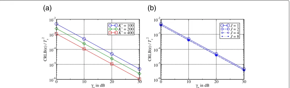
with f = expjΦ, α_l,J = l/J+(ε −s)/Ts. The start-ing phase Φ is generated randomly between 0 and 2π. As there is only a single-path, there are no excess delays and, thus, the channel memory length results inL = 9 (L = JL). In Figure 2, the normalized CRLB ofεfor the single-path channel is plotted over the PNR. In Figure 2a, the influence of the burst lengthKis shown for symbol-rate sampling (J = 1), whereas in Figure 2b the influence of the oversampling factorJis illustrated for a burst length of K = 100. In all cases, the CRLB decreases with the PNR and is much smaller than one, which corresponds to a small fraction of the squared symbol duration T_s2. This means that the estimation error is much smaller than the symbol duration Ts. The larger the burst length, the better the performance: The CRLB improves by approxi-mately 3 dB if the burst length is doubled (see Figure 2a). The same influence of the burst length is observed in all other channel models. Hence, only burst lengths of K = 100 are considered in the following if not stated otherwise. Furthermore, oversampling provides a slight performance gain as shown in Figure 2b: For all over-sampling factors J ≥ 2, the CRLBs are improved by approximately 0.8 dB in comparison to symbol-rate sam-pling. A similar behavior is observed for the remaining channel models as well, i.e., all oversampling factorsJ≥2 lead to same performance gain. Hence, onlyJ =2 is con-sidered subsequently. The question arises for what reason oversampling provides a performance gain? What is the difference between symbol-rate sampling and oversam-pling? In order to answer these questions, the CRLB for the single-path channel is examined in more detail. The starting point is the Fisher information matrix given in (25). In order to keep the following investigations man-ageable, two assumptions are applied which simplify the determination of the Fisher information matrix. First, white noise is assumed for all oversampling factors and, second, the burst length is assumed to be large. In this case, the inverse covariance matrix of the channel estima-tion error can be approximated by a scaled identity matrix

Cη−1 =XH0 Cn−1X0 ≈γ ·I (34)

with scaling factorγ = (K−L)/(Jσ_n2). This leads to an approximate Fisher information matrix

I(θ)≈2γ ·ReJ(θ)HJ(θ). (35) Hence, only the Jacobian matrix needs to be deter-mined. The partial derivatives of the channel coefficients are given by

∂hl

∂θ1 =

exp−α2_l,J

, ∂hl

∂θ2 =

j exp−α_l2_,J

,

∂hl

∂θ₃ =2f ·exp

−α_l2_,J

·αl,J.

0 10 20 30

γp in dB

10-6 10-5 10-4 10-3 10-2

CRLB(

ε

) /

Ts

2

K’ = 100

K’ = 200

K’ = 400

(a)

0 10 20 30

γp in dB

10-6 10-5 10-4 10-3 10-2

CRLB(

ε

) /

Ts

2

J = 1

J = 2

J = 4

J = 8

(b)

Figure 2Normalized CRLB ofεversus PNR for the single-path channel.(a)Influence of the burst lengthK(J₌1).(b)Influence of the oversampling factorJ(K=100).

Multiplying the Hermitian conjugate of the Jacobian matrix with the Jacobian matrix itself and taking the real part of the result leads to a Fisher information matrix of the following form:

I(θ)≈2γ · ⎡ ⎣A0 0A CB

B C D ⎤

⎦ (37)

with

A= L

l=0

exp

−α_l2_,J 2

, (38)

B=2 Ref L

l=0

exp

−α_l2_,J 2

·α_l,J, (39)

C=2 Imf L

l=0

exp−α2_l,J2·α_l,J, (40)

D=4|f|2 L

l=0

exp−α_l2_,J 2

·α2_l,J. (41)

Inverting the matrix in (37) results in

I(θ)−1≈ 1

2γ ·

1

A(AD−B2_−C2₎

⎡ ⎢ ⎢ ⎣

AD−C2 _{BC −AB}

BC AD−B2 −AC

−AB −AC A2

⎤ ⎥ ⎥ ⎦.

(42)

The CRLB of the sampling phase corresponds to the third main diagonal entry of the above matrix

CRLB(ε)

= I(θ)−1_3,3≈ 1 2γ ·

A AD−B2_−C2

= 1

8γ|f|2·

×

L

l=0

exp−α_l2_,J2

'

L

l=0

exp−α2_l,J2

( '

L

l=0

exp−α_l2_,J2·α2_l,J

(

−

'

L

l=0

exp−α_l2_,J2·αl,J

(2.

(43)

Since |f|2 _{is always one in the single-path channel,} the difference between symbol-rate sampling and over-sampling must depend somehow on the sums over the exponential terms and, thus, on the sampling phase itself. In Figure 3, the influence of the sampling phase on the approximate CRLB is illustrated: In Figure 3a, the approx-imate CRLB is plotted over the sampling phase ε for symbol-rate sampling and oversampling with J = 2 for

γ_p = 10 dB. For oversampling withJ = 2, the approx-imate CRLB is constant and does not depend on ε. In contrast, the approximate CRLB varies with the sampling phase for symbol-rate sampling. Thus, there is a con-siderable difference between symbol-rate sampling and oversampling. The same behavior can be observed for the average channel power divided by the oversampling factor,

1 JE

_L

l=0

|hl(θ)|2

= 1

JE _L

l=0

exp

α2_l,J

2

-0.5 -0.25 0 0.25 0.5 sampling phase ε / T

s

4.5e-04 5.0e-04 5.5e-04 6.0e-04 6.5e-04

CRLB(

ε

) /

Ts

2

J = 1

J = 2

(a)

-0.5 -0.25 0 0.25 0.5 sampling phase ε / T

s

0.98 0.99 1 1.01 1.02

power of the channel / J

J = 1

J = 2

(b)

Figure 3Influence of the sampling phase on the approximate normalized CRLB.(a)Approximate normalized CRLB ofεversus the sampling phase withγp=10 dB.(b)Average channel power divided by the oversampling factor vs. the sampling phase.

which corresponds to the numerator in (43). The average channel power according to (44) is plotted in Figure 3b: For oversampling with J = 2, the power of the chan-nel is constant and, thus, independent of the sampling phase. For symbol-rate sampling, in contrast, the power of the channel is a function of the sampling phase: The highest power is obtained forε=0 (perfect synchroniza-tion), while the smallest power occurs for |ε| = 0.5Ts. This means that non-perfect synchronization leads to a power loss concerning symbol-rate sampling. Similar results have already been reported by the authors in [6] for a rectangular and a root raised cosine pulse shape.

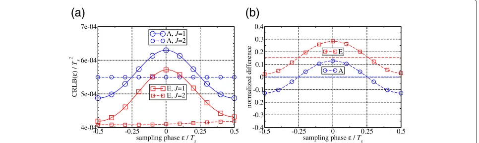
Now, it is clear that there is a considerable difference between symbol-rate sampling and oversampling. But the question remains: How does this difference lead to the observed performance gain of oversampling? In order to answer this question, it is necessary to return to the exact Fisher information matrix described by (25) and the cor-responding exact CRLB. How does the behavior of the CRLB change if the exact instead of the approximate ver-sion is taken into account? In Figure 4a, both types of the

CRLB are plotted over the sampling phase ε for K = 100, γ_p = 10 dB and J = 1, 2. The curves are labeled with “A” for approximate and “E” for exact. In order to have a closer look at the different behavior of the approx-imate and the exact CRLB, the normalized difference between the symbol-rate sampled and the oversampled CRLB according to

CRLB(ε)_J=1−CRLB(ε)_J=2

CRLB(ε)_J=1 , (45)

is plotted for each type in Figure 4b. For the approxi-mate and the exact CRLB, the shape of the corresponding curves is basically the same. The difference between the approximate CRLB and the exact CRLB lies in the fact that the curves of the exact CRLB are shifted downward with the shift for symbol-rate sampling being smaller than the shift for oversampling. This means that the curves of the normalized difference between the CRLBs are shifted upward. A slight deviation is observed in case of the

-0.5 -0.25 0 0.25 0.5 sampling phase ε / T_s

4e-04 5e-04 6e-04 7e-04

CRLB(

ε

) /

Ts

2

A, J=1 A, J=2

E, J=1 E, J=2

(a)

-0.5 -0.25 0 0.25 0.5 sampling phase ε / T_s

-0.4 -0.3 -0.2 -0.1 0 0.1 0.2 0.3 0.4

normalized difference

A E

(b)

exact CRLB for J = 2: In contrast to the approximate CRLB for oversampling, the exact CRLB for oversam-pling is not absolutely constant over the whole range of sampling phases, but it slightly increases forε ≥ 0 (see Figure 4a). This effect is due to the short burst length ofK = 100. For larger burst lengths (e.g.,K = 400), this effect is not present anymore and the exact CRLB for J = 2 is absolutely constant over the whole sam-pling phase range as well. The most interesting aspect is revealed by the mean of the normalized difference, which is shown as a straight line in Figure 4b. If white noise is assumed for all oversampling factors (“A”), then the mean of the normalized difference (45) equals zero in all cases. That means thaton average there is no dif-ference between symbol-rate sampling and oversampling such that the CRLBs determined via Monte Carlo simu-lations (with a random sampling phase) are the same. In case of colored noise (“E”), the mean of the normalized difference (45) is approximately 0.16 forK = 100, i.e., the exact CRLBs for symbol-rate sampling and oversam-pling differ on average by a small amount. This difference leads to the oversampling gain which has been observed in Figure 2b.

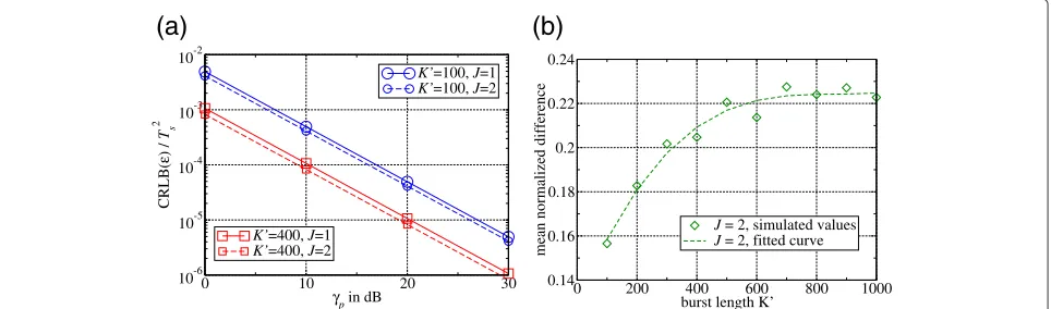
Last but not least, it is interesting to note that the mean of the normalized difference as well as the oversampling gain vary with the burst lengthK. In Figure 5, the influ-ence of the burst length K is examined in more detail: In Figure 5a, the CRLB of ε is plotted for symbol-rate sampling and oversampling with different burst lengths of K = 100 and K = 400. As already mentioned before, the performance gain of oversampling is approx-imately 0.8 dB forK = 100. For K = 400, this gain is increased to approximately 1 dB. For comparison, the mean of the normalized difference is plotted over the burst lengthKin Figure 5b. The circles denote the simu-lated values, while the dashed line corresponds to a fitted curve. It is observed that the mean normalized differ-ence increases with the burst length and saturates around

0.223, i.e., from approximately K = 800 upward the mean normalized difference is constant. The mean nor-malized difference for K = 400 is approximately 0.2. Interestingly, the ratio of the performance gains corre-sponds to the ratio of the mean normalized differences: 0.8/1 dB = 0.8 = 0.16/0.2. Thus, the mean of the nor-malized difference translates into the performance gain with a positive factor. As the mean normalized difference saturates around 0.223, the maximum achievable over-sampling gain is approximately 1.115 dB in a single-path channel.

Two-path channels

Two-path channels represent the simplest form of a mul-tipath channel. Since block fading is assumed, a two-path channel can be fully characterized according to

hl=a1exp

jΦ1

exp #

− $

lT +ε−s Ts

%2&

+a2exp

jΦ2

×exp #

− $

lT +ε−s−ν₂

Ts

%2& .

(46)

By means of the two-path channel models, the influence of different channel characteristics such as the excess delay

ν2, power ratio P = a21/a22, and phase offset Φ =

Φ2−Φ1between the two propagation paths can be inves-tigated. The maximum possible excess delay is fixed to

ν₂max = 2Ts, which leads to a channel memory length ofL = 11 (L = JL). At first, the CRLB of ε is exam-ined over PNR, where the power ratio and the phase offset are generated randomly in the intervals [0.1, 10] and [0,2π], respectively. Concerning the excess delay, two different scenarios are considered: one with small excess delays (ν2/Ts ∈[ 0.05, 1]) and one with large excess delays (ν2/Ts ∈[ 1, 2]). The corresponding CRLBs for different

0 10 20 30

γp in dB

10-6 10-5 10-4 10-3 10-2

CRLB(

ε

) /

Ts

2

K’=100, J=1

K’=100, J=2

K’=400, J=1

K’=400, J=2

(a)

0 200 400 600 800 1000 burst length K’

0.14 0.16 0.18 0.2 0.22 0.24

mean normalized difference

J = 2, simulated values

J = 2, fitted curve

(b)

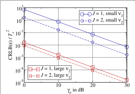
oversampling factors are shown in Figure 6. The overall performance decreases with respect to the LOS chan-nel (as expected) but the oversampling gain increases. Both, the overall performance and the oversampling gain, depend on the channel model: The smaller the excess delay, the worse is the CRLB and the larger is the over-sampling gain. For the channel with small excess delay, the gain is approximately 6.5 dB, whereas it is only 2.6 dB for the channel with large excess delay. In order to have a closer look at this dependence, the CRLBs are determined over the excess delay for a fixed PNR (γ_p = 10 dB). Simi-larly, the influence of the phase offsetΦand the power ratioPis investigated.

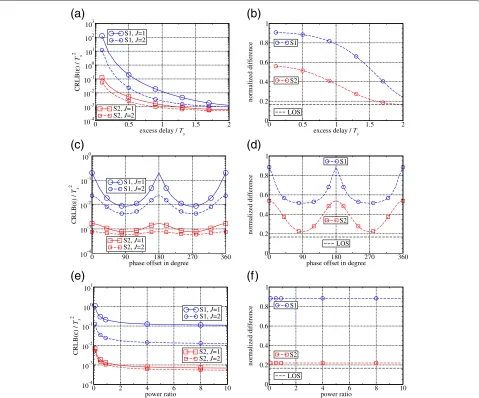
In contrast to the LOS channel, the approximate Fisher information matrix according to (35) and the correspond-ing approximate CRLB are not considered here. Due to the increased size of the Fisher information matrix (6×6 instead of 3×3), the resulting formula for the approximate CRLB consists of many different terms and is, therefore, less concise than in the case of the LOS channel. Two basic simulation setups are applied, whose characteris-tics are tabulated in Table 1. The parameter of interest is varied, while the other parameters are fixed to the val-ues given in Table 1. The corresponding CRLBs and their normalized differences according to (45) are shown on the left-hand side and on the right-hand side of Figure 7, respectively. The curves are labeled with “S1” for the first setup and “S2” for the second setup. The mean normal-ized difference of the LOS channel (forK=100) is given for comparison in Figure 7b,d,f since it corresponds to a lower bound concerning the normalized difference of the two-path channels. In the first row of Figure 7, the influ-ence of the excess delayν2 is illustrated for both setups, while the influence of the phase offsetΦand the power ratioP are shown in the second and third row, respec-tively. The overall performance and the oversampling gain

0 10 20 30

γp in dB

10-5 10-4 10-3 10-2 10-1 100 101

CRLB(

ε

) /

Ts

2

J = 1, small ν₂ J = 2, small ν₂

J = 1, large ν₂ J = 2, large ν₂

Figure 6Normalized CRLB ofεversus PNR for the two-path channels with small and large excess delayν2.

Table 1 Basic simulation setups for the two-path channel models

Parameter Setup 1 Setup 2

ν2/Ts 0.5 1.5

P 1.0 5.0

Φ 0◦ 90◦

strongly depend on the simulation setup and the channel characteristic of interest. It is obvious that the first setup corresponds to a kind of worst case concerning param-eter estimation, whereas the second setup represents a kind of best case scenario. For the first setup, overpling can provide a significant gain over symbol-rate sam-pling. This gain isnotinfluenced by the power ratio (see Figure 7f ), while itmainlydepends on the excess delayν₂

(see Figure 7b): The smaller the excess delay, the larger is the oversampling gain. Hence, oversampling proves espe-cially helpful in dense multipath scenarios. Furthermore, the phase offsetΦhas a significant impact on the over-sampling gain, which is highest when both propagations paths have the same or the opposite phase (see Figure 7d). As mentioned above, the normalized difference trans-lates into the oversampling gain with a positive factor. Thus, the larger the normalized difference, the larger is the oversampling gain.

Figure 7 does not only illustrate the dependence of the oversampling gain on the channel characteristics, but gives also an insight into the relation between these char-acteristics and the overall performance. With decreasing excess delayν₂, the CRLB increases as it becomes more difficult to separate the two propagation paths. Similarly, the CRLB is worst if the paths are in phase (Φ = 0◦) or have an opposite phase (Φ =180◦). The smaller the power ratio P, the smaller is the amplitude of the first path in comparison to the second path and the more likely it is that the delay of the first path, namely the sampling phase, is estimated wrongly. Thus, the influence of the channel characteristics on the overall performance can be summarized as follows: Dense multipath scenarios with similar or opposite phases and a small power ratio are most challenging. The more challenging it is to estimate the sampling phase, the higher is the gain due to oversam-pling. Hence, the application of oversampling (withJ=2) is highly recommended.

WINNER channels

0 0.5 1 1.5 2 excess delay / T_s

10-4 10-3 10-2 10-1 100 101 102 103

CRLB(

ε

) /

Ts

2

S1, J=1 S1, J=2

S2, J=1 S2, J=2

(a)

0 0.5 1 1.5 2

excess delay / T_s

0 0.2 0.4 0.6 0.8 1

normalized difference

S1

S2

LOS

(b)

0 90 180 270 360

phase offset in degree 10-4

10-3 10-2 10-1 100

CRLB(

ε

) /

Ts

2 S1, _S1, J_J=1₌₂

S2, J=1 S2, J=2

(c)

0 90 180 270 360

phase offset in degree 0

0.2 0.4 0.6 0.8 1

normalized difference

S1

S2

LOS

(d)

0 2 4 6 8 10

power ratio 10-4

10-3 10-2 10-1 100 101

CRLB(

ε

) /

Ts

2

S1, J=1 S1, J=2

S2, J=1 S2, J=2

(e)

0 2 4 6 8 10

power ratio 0

0.2 0.4 0.6 0.8 1

normalized difference

S1

S2

LOS

(f)

Figure 7Comparison of normalized CRLBs and the normalized difference between CRLBs for different channel characteristics with γp=10dB.The curves are labeled with “S1” for the first setup and “S2” for the second setup.(a)Normalized CRLB ofεversus excess delay.(b) Normalized difference of CRLBs versus excess delay.(c)Normalized CRLB ofεversus phase offset.(d)Normalized difference of CRLBs versus phase offset.(e)Normalized CRLB ofεversus power ratio.(f)Normalized difference of CRLBs versus power ratio.

(SISO) is considered here. Two types of channel models are presented in [33]: The generic model, that is suited for system level simulations, and theclustered delay line (CDL)model, that is reduced in complexity for fast link level simulations. In this contribution, the CDL models are utilized. The parameters of the CDL models like the excess delay or the average power of a multipath ponent are fixed and tabulated. A single multipath com-ponent is calledcluster in [33]. With the Gaussian pulse shape in (30) and the block fading assumption, the channel coefficients for WINNER channel models withIclusters are given as

hl= I

i=1 fi·exp

# −

$

lT +ε−s−ν_i

Ts

%2&

, (47)

where the complex amplitudes fi are determined by the superposition ofR=20 rays according to

fi=Ai· 1

√

R R

r=1

expjΦi,r. (48)

If a LOS component is present, the first cluster consists of R = 21 rays. Each cluster is assigned a normalized amplitudeAithat is computed from the tabulated cluster powersPias

Ai= ) * *

+_Pi,I i=1

Pi (49)

for each ray in every cluster. Three different WINNER channel models are considered in this paper:typical urban micro-cell(B1-LOS),large indoor hall(B3-LOS) and typ-ical urban macro-cell(C2-LOS). For an exact description of these scenarios and the corresponding parameter tables please refer to [33].a The most important parameters of the WINNER channel models are summarized in the upper part of Table 2. In addition to the number of clus-tersI and the number of parametersP, the Rician factor KRas well as the excess delaysν2andνI are listed. Fur-thermore, the minimum delay difference, min{ν_i−ν_i−1}, and the average delay difference, E{ν_i−ν_i−1}, between neighboring paths is determined. For the minimum delay difference, the cluster number for which this difference occurs is given. Until now, only normalized excess delays

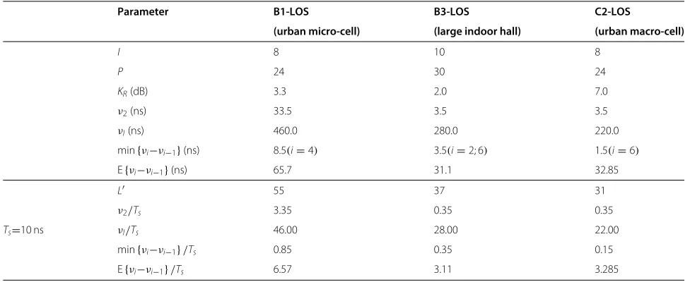
ν2/Tshave been considered. Thus, the preceding results are valid for any choice of the symbol duration Ts. In case of the WINNER channel models, the excess delays are given as absolute values in ns. Hence, the simulation results depend on the choice of the symbol duration Ts. Here,Ts=10 ns is considered. In the lower part of Table 2, the channel memory lengthL for symbol-rate sampling (L=JL) as well as the relative excess delays and relative delay differences forTs=10 ns are tabulated.

In the WINNER channel models, parameter estimation is much more challenging in comparison to the two-path channel models since a much larger number of prop-agation paths I>2 is considered. Thus, the dimension of the estimation process P=3I increases significantly. However, the relationships observed for the two-path channels are the basis for more complex channel mod-els with an arbitrary number of propagation paths like the WINNER channel models. In this case, the mutual rela-tionship between all paths determines the performance, where the relationship between the first and the second

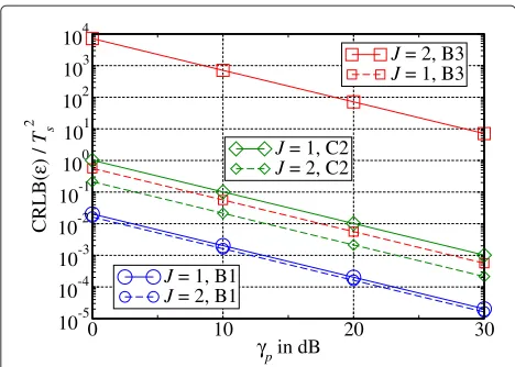
path is of special importance. A performance progno-sis can be given based on the results obtained for the two-path channel models: Dense multipath scenarios with similar or opposite phases and a small power ratio are most challenging. Due to the superposition of several rays per cluster with random starting phases, the phase off-sets and power ratios of all paths are random and can not be influenced. Nevertheless, the Rician factor is a valuable indicator since it is defined as the average power ratio of the LOS path and the scattered components. The smaller the Rician factor, the smaller is the average LOS power and the worse the performance should be. From this point of view, the B3-LOS channel is most challenging. Fur-thermore, the relative excess delays and delay differences are of interest. Especially, the relative excess delay of the first multipath component ν2/Ts is important since the corresponding pulse overlaps the most with the LOS com-ponent. For Ts=10 ns, the relative excess delays of the first multipath component are in a reasonable range. The same is valid for the relative minimum delay differences. Again, the B3-LOS is most challenging with respect to delay differences because a very small delay difference of 3.5 ns occurs twice. Taking all parameters into account, the worst performance is expected for the B3-LOS chan-nel (large indoor hall), whereas the best performance is predicted for the B1-LOS channel (urban micro-cell). The CRLBs of all three WINNER channels for symbol-rate sampling and oversampling with J = 2 are shown in Figure 8. The above performance prediction is met by all simulation results: The best and worst performance is obtained for the B1-LOS and the B3-LOS channel, respec-tively. For oversampling with J = 2 (dashed lines), the CRLBs are even better than the corresponding CRLB for the two-path channel with small excess delay. The per-formance of the B1-LOS channel is even similar to the

Table 2 Selected parameters of the WINNER channels

Parameter B1-LOS B3-LOS C2-LOS

(urban micro-cell) (large indoor hall) (urban macro-cell)

I 8 10 8

P 24 30 24

KR(dB) 3.3 2.0 7.0

ν2(ns) 33.5 3.5 3.5

νI(ns) 460.0 280.0 220.0

min_{νi−νi−1}(ns) 8.5(i₌4) 3.5(i₌2; 6) 1.5(i₌6)

E_{νi−νi−1}(ns) 65.7 31.1 32.85

L 55 37 31

ν2/Ts 3.35 0.35 0.35

Ts=10 ns νI/Ts 46.00 28.00 22.00

min{νi−νi−1}/Ts 0.85 0.35 0.15

0 10 20 30 γp in dB

10-5 10-4 10-3 10-2 10-1 100 101 102 103 104

CRLB(

ε

) /

Ts

2

J = 1, B1 J = 2, B1

J = 2, B3 J = 1, B3

J = 1, C2 J = 2, C2

Figure 8Normalized CRLB ofεversus PNR for the WINNER channels B1, B3 and C2 withTs=10ns.

performance of the two-path channel with large excess delay. In contrast, a significant performance degradation is observed for symbol-rate sampling. For the B3-LOS chan-nel, the normalized CRLB atγp = 0 dB is very high with a value close to 104_{. This means that oversampling gains} larger than 30 dB are possible in case of the WINNER channel models. Hence, it is highly recommended to apply oversampling withJ=2 because accuracies well below the symbol duration can only be obtained for oversampling.

The symbol duration of Ts = 10 ns has been chosen for the simulations in order to achieve reasonable val-ues for the relative excess delays. With increasing symbol duration Ts, the relative excess delays and delay differ-ences decrease. Very small delay differdiffer-ences lead to ill-conditioned (or even rank-deficient) Fisher information matrices, that are difficult to invert. In order to avoid a complete failure of the matrix inversion, singular value decomposition as described in [32, p. 62ff.] can be applied. However, the corresponding CRLBs degrade significantly if the relative delay differences become too small. In this case, the channel models are not adequate anymore and should be revised because neighboring clusters are not resolvable by any means and act like additional rays that contribute to a single cluster. This means, that clusters with nearly the same relative excess delay should be com-bined to a single cluster. In this way, the number of clusters is reduced, the new clusters are resolvable and meaningful CRLBs can be determined again.

Impact of the performance limits for CPE on the overall positioning process

As already mentioned in the introduction part of this article, positioning is typically performed in two steps, namely parameter estimation and position estimation. Until now, only the first step (CPE) has been examined. In the following, the impact of the performance limits

for CPE on the second step is discussed. Hence, sev-eral links between different reference objects (ROs) and a mobile station (MS) in a certain geometrical setup have to be taken into account. For a better understanding, the positioning problem for localization based on the ToA is shortly introduced and a corresponding CRLB is derived. Two-dimensional positioning is considered for that pur-pose, i.e.,at leastthree ROs are needed to determine the position of the MS. An extension to three-dimensional localization is straight forward.

The MS’s position, that shall be estimated from the ToAs, is denoted by p=[p1,p2]T=[x,y]T, while the known locations of the ROs are denoted by

p_b=[pb,1,pb,2]T=[xb,yb]T, 1≤b≤B, where B is the number of reference objects. The true distance between the MS and thebth RO is a nonlinear function of the cur-rent MS’s positionpand can be determined according to

db(p)=

-(x−xb)2+

y−yb

2

. (50)

These distances are estimated via the ToAs τˆ_b,1

based on dˆb= ˆτb,1·c, where c is the speed of light. The estimated distances d=ˆ [d1,ˆ . . .,dˆB]T are called pseudoranges since they consist of the true dis-tances d(p)=[d1(p),. . .,dB(p)]T and estimation errors

e=[e1,. . .,eB]T with covariance matrix Ce=diag

σ_e2₁,. . .,σ_e2_B:

ˆ

d=d(p)+e. (51)

Again, an ML estimator can be applied to estimate the position of the MS:

ˆ

p=arg min

˜

p

ˆ

d−d(p˜) T

C−e1

ˆ

d−d(p˜)

=arg min

˜

p

Ω_dˆ(p˜)

(52)

Similar to the ML estimator for CPE, the metricΩ_dˆ(p˜)

for position estimation is nonlinear due to the nonlinear distance function (50). Hence, an optimization algorithm has to be applied similar to the case of CPE. Often, a Gauss-Newton approach known asTaylor seriesalgorithm [34,35] is utilized for positioning. But for positioning, there are additionally some approximative, non-iterative estimators like theweighted least-squaresalgorithm avail-able [36,37].