Concepts for the Temporal Characterization
of Short Optical Pulses
Christophe Dorrer
Bell Laboratories, Lucent Technologies, 791 Keyport-Holmdel Road, Holmdel, NJ 07733, USA Email:[email protected]
Ian A. Walmsley
Clarendon Laboratory, Parks Road, Oxford OX1 3PU, United Kingdom Email:[email protected]
Received 1 April 2004; Revised 15 September 2004
Methods for the characterization of the time-dependent electric field of short optical pulses are reviewed. The representation of these pulses in terms of correlation functions and time-frequency distributions is discussed, and the strategies for their characteri-zation are explained using these representations. Examples of the experimental implementations of the concepts of spectrography, interferometry, and tomography for the characterization of pulses in the optical telecommunications environment are presented.
Keywords and phrases:optical pulse characterization, time-frequency distribution, Wigner function, spectrogram, tomography,
interferometry.
1. INTRODUCTION
Ultrashort optical pulses are used in areas of science and engineering as diverse as spectroscopy, medical research, plasma physics, quantum optics, and optical telecommuni-cations. In optical telecommunications, information is en-coded in the amplitude and/or phase of an optical wave [1]. While information encoding in digital telecommunications is based on a finite number of values of a physical quantity (e.g., the presence or absence of energy in a given bit slot), the ability to measure in detail the waveform of the optical wave itself is crucial for optimizing the properties of the systems that generate the signal, and understanding the linear and nonlinear properties of the systems through which the pulses propagate. This information is critical in developing strate-gies to overcome the current limitations of current opti-cal networks. For example, dispersion management compen-sates for the chromatic dispersion induced by linear propaga-tion and can also be used to mitigate nonlinear effects. Sim-ilarly, the phase distortion imposed on a pulse by the mod-ulators used in carving the pulse out of a cw- or quasi-cw source can impact the propagation of the pulse. Finally, mea-surements of the electric field can be used to characterize the linear or nonlinear properties of a device. There are various approaches for temporal waveform measurements. We only consider here techniques that provide self-referencing char-acterization of an unknown pulse or a train of unknown but
identical pulses, that is, that do not use a well-characterized pulse as a reference. While test-plus-reference techniques, such as spectral interferometry [2,3,4], can be easier to im-plement in some cases, they require a well-characterized ref-erence pulse mutually coherent with the pulse under test. Al-though this can be difficult to achieve over long distances, they have been used to characterize pulses in the telecommu-nication environment [5]. We will not deal either with sam-pling techniques. These techniques can provide samples of the temporal intensity of a source by fast photodetection and electronics or by nonlinear interaction with a short sampling pulse (nonlinear optical sampling) [6]. The technique of lin-ear optical sampling [7] is also sensitive to the electric field of the source (i.e., it can measure samples of the intensity and phase of the source under test), and can therefore be used to measure constellation diagrams [8]. These techniques are particularly useful when dealing with a data-encoded opti-cal source because of the randomness of the data stream, but they constitute a class of their own that is beyond the scope of this paper. The concepts presented here apply generally to the characterization of the temporal electric field of short optical pulses, although the details of experimental implementations are strongly dependent upon the domain of application.
so their output contains no information about the phase of the incident radiation. To overcome these limitations, a com-bination of ancillary filters can be used. The data are sim-ply the photocurrent recorded by a time-integrating detector as a function of the parameters of the filters. These might be, for example, the passband frequency for a spectrometer (a time-stationary linear filter), the modulation index for a phase modulator (a time-nonstationary linear filter), or the relative delay between the pulse under test and the mod-ulation induced by an electroabsorption modulator (also a time-nonstationary linear filter).
There are a number of quite general strategies for char-acterizing the electric field of an optical pulse using such fil-ters. These belong to one of three categories: spectrographic, tomographic, or interferometric. The categories are distin-guished by the procedure required for reconstructing the am-plitude and the phase of the field from the recorded data [9, 10]. Since the analytic signal of the field is a complex function of one real variable, time, with finite support, the data must contain a finite set of complex numbers sampling the field at a finite set of time points, or equivalently a finite set of frequency points. It can sometimes be fruitful, how-ever, to reconstruct pulses by sampling a time-frequency rep-resentation of the pulse (or its equivalent correlation func-tion). In this case a two-dimensional set of data is obtained, from which an inversion algorithm reconstructs an estimate of the field. This is typically the case for spectrography, which makes use of a time-frequency distribution, and requires so-phisticated iterative data inversion algorithms to reconstruct the field. Tomography also requires a large data set, in the form of a large number of modulated pulse spectra, but the inversion is direct (noniterative). Interferometry, in contrast, measures only a one-dimensional data set and uses direct data inversion to reconstruct the field.
In this paper, we provide examples of each of these methods that are relevant to optical telecommunications. In Section 2, we first discuss the representation of the electric field of a pulse or train of pulses, and how the various mea-surement techniques sample the field. Then, inSection 3, we illustrate both the data acquisition and inversion for each method.
2. REPRESENTING LIGHT PULSES
The fundamental quantity describing an isolated, individual pulse of light is the real electric field. This is a function of time and space, or equivalently frequency and wavevector. The spatial dependence of the field is often assumed uniform. This assumption is valid for optical fiber-based telecommu-nications if the field occupies the lowest-order mode of the fiber. Therefore in this paper, we concentrate on determining the time dependence of the electric field.
In practice, it is often difficult to characterize a single pulse, and one deals with a train of pulses instead of a single pulse. One must be careful in specifying a field for such an ensemble. If all of the pulses in the train are identical, the en-semble is deemed coherent, and the underlying electric field
of an individual remains the quantity of interest. If, on the other hand, the electric field is stochastic, fluctuating from pulse to pulse, the ensemble is said to be partially coherent. When this is the case, the amplitude and phase of the electric field of an individual pulse brings little information on the train of pulses, and pulse characterization involves measure-ments of the statistical properties of the ensemble, for exam-ple via the two-time or two-frequency correlation function. We note that a data-modulated train of pulses is not coher-ent if the data modulation is random (which is the case for a deployed communication system).
2.1. Describing an optical pulse by its analytic signal
The real electric field, ε(t), underlying an optical pulse is twice the real part of its analytic signal E(t) : ε(t) = 2×
Re[E(t)]. The analytic signal is the single-sided inverse Fourier transform of the Fourier transform of the field,
E(t)=√1 2π
∞
0 dωε(ω) exp[−iωt], (1)
where
ε(ω)=√1
2π
∞
−∞dt ε(t) exp[iωt]. (2)
The electric field is considered to have compact support in the time domain, and is further assumed to have no spectral component atω=0 soε(0)=0 (since a pulse propagating in a charge-free region of space has no dc spectral component, the electric field must have zero area). The analytic signal is complex and therefore can be expressed uniquely in terms of an amplitude and phase:
E(t)=E(t)expiφt(t)
expiφ0
exp−iω0t
, (3)
where|E(t)|is the time-dependent envelope,ω0is the carrier
frequency (usually chosen near the center of the pulse spec-trum),φt(t) is the time-dependent phase, andφ0a constant.
The square of the envelope,|E(t)|2, is the time-dependent
intensity of the pulse which could be measured by a detec-tor of sufficient bandwidth. The time-dependent phase ac-counts for the occurrence of different frequencies at different times, and the instantaneous frequency is usually defined as
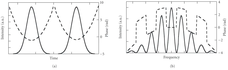
−∂φt/∂t. As an example,Figure 1shows the temporal inten-sity and phase of a pair of chirped Gaussian pulses. The time-dependent phase structure is indicative of a variation of the instantaneous frequency across the pulse.
The frequency representation of the analytic signal is the Fourier transform ofE(t),
E(ω)=E(ω)·expiφω(ω)
= √1
2π
∞
−∞dt E(t) exp[iωt] =
ε(ω), ω >0, 0, ω≤0.
In
te
nsit
y
(a.u.)
Time
10
5
0
−5
Phase
(r
ad)
(a)
In
te
nsit
y
(a.u.)
Frequency
4 2 0
−2
−4
Phase
(r
ad)
(b)
Figure1: Intensity and phase (resp., continuous and dashed line) of a pair of chirped Gaussian pulses in (a) the temporal domain and (b) the spectral domain.
Here|E(ω)|is the spectral amplitude andφω(ω) is the spec-tral phase. The square of the specspec-tral amplitude,|E(ω)|2, is
the spectral intensity. Strictly speaking this quantity is the spectral flux—the quantity measured in the familiar way by means of a spectrometer followed by a photodetector. The spectral phase describes the relative phases between each of the frequencies, and the group delay for frequencyωis usu-ally defined as∂φω/∂ω.
The sampling requirement for the reconstruction of the electric field is given by the Whittaker-Shannon theorem [11], which asserts that if the field has compact support in the time domain over a range∆t, then a sampling ofE(ω) at the Nyquist frequency rate of 2π/∆tis sufficient for
reconstruct-ing the analytic signalE(t) and consequently the electric field
ε(t) exactly.
Figure 1shows the spectral intensity and spectral phase of the chirped pair of Gaussian pulses. The spectral fringes have a period of the inverse of the temporal separation of the pair of pulses. While the spectrum can reveal some properties of the waveform, both the spectral intensity and phase must be measured to fully characterize the electric field.
2.2. The two-time correlation function and its phase-space representations
If a measurement relies on averaging the detected signal over a train of pulses, then it is necessary to define the properties of the pulses in a different way. Although it is formally quite difficult to formulate rigorously even the simplest of con-cepts, such as the spectrum [12], for a nonstationary field, a simple-minded approach can be fruitful. If each pulse in the train is an independent realization of a stochastic ensem-ble, then the time average is equivalent to an ensemble av-erage by definition. This enables the coherence of the train to be defined operationally in a reasonable way. It is impor-tant, though, to realize that the electric field amplitude and phase of an individual pulse does not bring significant infor-mation about the train of pulses and pulse characterization efforts must ultimately be directed toward measurement of the ensemble statistics.
The simplest quantity that quantifies the statistical prop-erties of the ensemble is the nonstationary two-time field correlation function
C t1,t2
=E t1
E∗ t2
, (5)
where the angle brackets indicate an average over the ensem-ble of pulses, each of the electric fields being defined with respect to a local time frame. With this definition of the en-semble, we do not need to adopt procedures along the lines of those developed by Wiener and Khintchine [13] to define the correlation function.
C(t1,t2) provides a quantitative description of
fluctua-tions from pulse to pulse in the electric field at timest1
rela-tive to those at timest2. This is a complete description of the
pulse ensemble so long as the fluctuations obey normal (or Gaussian) statistics. If not, then it is the simplest of a hierar-chy of multitime correlation functions defining the ensem-ble. Furthermore, for a train of identical pulses,C(t1,t2)
fac-torizes intoE(t1)E∗(t2) and the electric field amplitude and
phase are readily obtained.
It is frequently useful to work with a variation of the correlation function that uses a two-dimensional space of time and frequency—the chronocyclic phase-space. The in-tuitive concept of chirp (i.e., time-dependent frequency in the pulse) can be most easily seen within this space. The rela-tionships between the two-time correlation function and the chronocyclic (time/frequency) and frequency-domain repre-sentations of the ensemble may be derived by rewriting (5) in terms of a center-time coordinate,t, and a difference-time coordinate,∆t:
C(t,∆t)=C t1,t2
, (6)
wheret = (t1+t2)/2 and∆t = t1−t2. The two-frequency
field correlation function is obtained by taking the two-dimensional Fourier transform of the two-time correlation function
C(∆ω,ω)= 1 2π
ω
t
(a)
ω t
(b)
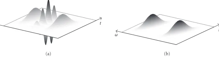
Figure2: Wigner function of a pulse with (a) linear chirp and (b) quadratic chirp.
ω
t
(a)
ω t
(b)
Figure3: Wigner function of the pair of chirped Gaussian pulses when the two pulses are (a) mutually coherent and (b) mutually incoherent.
The center-frequency and difference-frequency coordinates in (7) are given byω=(ω1+ω2)/2 and∆ω=ω1−ω2,
respec-tively. The pulse ensemble may also be represented within the chronocyclic phase spaces defined by the complimentary variablest,ωand∆ω,∆t. The chronocyclic Wigner function,
W(t,ω), and ambiguity or Wigner characteristic function,
A(∆ω,∆t), provide two particularly useful descriptions of the pulse train statistics in these spaces. The relationship between the various representations of the correlation function has been discussed in the context of spatially localized fields in [14], and in the context of signal analysis in [15]. Chrono-cyclic phase-space distributions have found increasing appli-cation in ultrafast optics. The Wigner function has been de-scribed in [16,17,18], and the Page distribution in [19]. An-other distribution of interest is the ambiguity function that is used in radar technology [20]. These functions are also used in many areas of physics and engineering, and their relations and properties are discussed in [21]. The Wigner function is obtained by taking the one-dimensional Fourier transform ofC(t,∆t) over the time-difference coordinate
W(t,ω)= √1
2π
d∆t C(t,∆t) exp[iω∆t], (8)
whereas the ambiguity function is obtained fromC(t,∆t) by performing the Fourier transform over the average-time co-ordinate
A(∆ω,∆t)=√1
2π
dt C(t,∆t) exp[i∆ωt]. (9)
These representations are uniquely related to one another by Fourier transformations. The Wigner function has many in-teresting properties, for example, the ability to represent a
chirp, as can be seen in Figure 2a. It is a real, but not nec-essarily positive function, which complicates its interpreta-tion as a density funcinterpreta-tion in the time-frequency space. For example, the Wigner function of a Gaussian pulse with a quadratic chirp (i.e., a third-order spectral phase), as dis-played inFigure 2b, is negative over a significant portion of the chronocyclic space. An example of the Wigner function of the pair of chirped Gaussian pulses inFigure 1is shown in Figure 3a. The side lobes are the phase-space representations of the individual pulses, and the cross-terms between the two fields lead to a central feature with fringes that indicate that the pulses have a definite phase relation to one another—they are coherent. The Wigner function for an incoherent pair of pulses is also show in Figure 3b. In this case the ensemble has a random phase between the pair, which causes a wash-ing out of the interference pattern when the signal is averaged over the ensemble. The coherence can be quantified using the Wigner function, as explained in the next section.
Information regarding the shapes of ultrafast optical pulses is generally inferred from the output of a square-law detector after some filtering. Therefore it is of practical inter-est to inter-establish the relationship between measurable detector output and the various descriptions of the pulse ensemble. The average pulse time-dependent intensity is obtained from the two-time correlation function by setting∆t = 0. Alter-natively, it is a projection of the Wigner function onto the frequency axis, or the Fourier transform of the∆t=0 line of the ambiguity function
I(t)=C(t, 0)
=
dω W(t,ω)
=
d∆ω A(∆ω, 0) exp[−i∆ωt].
Furthermore, the average pulse spectral intensity is obtained from the two-frequency correlation function by setting∆ω=
0, or by projecting the Wigner function onto the frequency axis, or by taking the Fourier transform of the∆ω=0 line of the ambiguity function:
I(ω)=C(0,ω)
=
dt W(t,ω)
=
d∆t A(0,∆t) exp[−i∆tω].
(11)
It is important to recognize that the various time-frequency distributions and their relations are central to the character-ization of pulses in the optical domain, since they are sim-ply related to the measured data. In optics, direct measure-ment of the waveform is not possible. This is in contrast to the more usual application of these distributions in signal processing, where they are commonly used as mathematical tools for signal representation, for example, to track the pres-ence of various instantaneous frequencies in a known (mea-sured) sound waveform.
2.3. The integral degree of coherence: when is a pulse field useful?
Since a field amplitude and phase may be defined in a unique way only for identical pulses, it is important to quantify the degree to which the pulses in the ensemble are alike. A useful quantity for this purpose is the integral degree of coherence,
µ. µis readily derived from the time-domain analogue of Born and Wolf ’s [13] degree of coherenceγ(t+∆t/2,t−∆t/2), defined as
γ(t+∆t 2 ,t−
∆t
2 )=
C(t,∆t)
C(t+∆t/2, 0)C(t−∆t/2, 0)1/2. (12) Using the Schwarz inequality, it is straightforward to show that 0 ≤ |γ(t+ ∆t/2,t −∆t/2)| ≤ 1. Consider the n -dimensional vectorsaandb, with components{ai}and{bi} wherei∈(1,n). Then
0≤
n
i=1
a∗ibi 2 ≤ n
i=1
a∗i ai
n
i=1
b∗i bi
. (13)
Allowingai=Ei(t−∆t/2)/√nandbi=Ei(t+∆t/2)/√n, that is, theith realization of the field amplitude at timest−∆t/2 andt+∆t/2, respectively, it is clear that
0≤1
n
n
i=1
E∗i
t−∆t
2
Ei
t+∆t 2 2 ≤ 1 n n
i=1
E∗i
t+∆t 2
Ei
t+∆t 2 × 1 n n
i=1
Ei∗
t−∆t
2
Ei
t−∆t
2
.
(14)
In the limit thatn→ ∞, the summations in (14) lead to an average over the ensemble and the inequality simplifies to
0≤C(t,∆t)2≤C
t+∆t 2, 0
C
t−∆t
2 , 0
. (15)
The upper and lower bounds on the degree of coherence fol-low from (15). However, it is difficult to determine γ(t+ ∆t/2,t−∆t/2) experimentally since it becomes singular for times at whichC(t,∆t) is zero. A practically more useful def-inition is offered by integrating equation (15) over the entire
t,∆tspace, and dividing by the quantity on the right-hand side, leading to the integral degree of coherence,µ,
0≤µ=
dt d∆tC(t,∆t)2
dt C(t, 0)2 ≤1. (16)
Equivalent relations follow for the frequency domain and chronocyclic representations, for example, in the case of the ambiguity function
µ=
d∆t d∆ωA(∆ω,∆t)2
A(0, 0)2 . (17)
An integral degree of coherence less than one corre-sponds to a partially coherent train in which the pulse shape and/or phase fluctuate, in which case C(t,∆t) is the funda-mental quantity of interest. Whenµ=1 the ensemble is said to be fully coherent (the pulses in the ensemble are identi-cal within a constant phase factor) andC(t,∆t) factorizes. In the latter case the electric field becomes the fundamental quantity of interest and is readily retrieved from the two-time correlation function using
E(t)=C(t, 0), (18)
and witht2held fixed,
ArgE(t)=tan−1
ImC t+t2
/2,t−t2
ReC t+t2
/2,t−t2
+φ0, (19)
whereφ0is an undetermined constant. For example, the
For a coherent train of pulses, (18) and (19) reveal that the electric field is retrieved from a single line of the correla-tion funccorrela-tion. Hence, if the ensemble is assumed a priori to be coherent, the amount of collected data can be greatly re-duced. This is a luxury afforded only to measurement tech-niques that directly measure one of the correlation func-tions.
2.4. Measurement strategies
The electric field of optical pulses can be characterized us-ing various strategies, derived from, and with implications for, other measurement problems, such as wavefront diag-nosis and quantum state reconstruction. These strategies can be organized into phase-space techniques, that is, techniques that attempt to measure either the Wigner or ambiguity function by exploring the entire two-dimensional chrono-cyclic phase space, and direct techniques, that obtain the elec-tric field of a coherent field from a single slice of a second-order correlation function.
The minimal requirement for the complete exploration of the chronocyclic space required in phase-space techniques is the presence of two filters. The analysis details of phase-space techniques are found in [9]. There are two subclasses of phase-space techniques; those that make simultaneous mea-surements of the complementary variables in an attempt to reconstruct one of the phase-space distributions, and those that record marginals of the Wigner function after rotation in the phase space, from which the Wigner function can be ob-tained. The former method is known as spectrographic while the latter is referred to as tomographic. Spectrography is dis-cussed in Sections3.1and3.2, and tomography is discussed in Sections3.5and3.6.
In contrast, direct techniques do not require this com-plete exploration of the phase space occupied by the correla-tion funccorrela-tion. This is a significant advantage of direct tech-niques compared to phase-space techtech-niques. Moreover, if the pulse train is assumed a priori to consist of identical pulses, as is most always assumed in reconstructing pulses from spec-trographic or tomographic data, only one slice of the corre-lation function is required to obtain the amplitude and phase of the electric field [10]. Such slices are precisely what is mea-sured in interferometry. This is usually achieved by mixing the field under test with a modified version of itself, or more generally by mixing two modified versions of the field un-der test. Thus, while phase-space techniques must explore the entire chronocyclic space even when the electric field is the fundamental quantity of interest, direct techniques need only return a single slice of the correlation function in or-der to construct the simpler quantity. Roughly speaking, if one wishes to reconstruct the field atNtime points, then at least 2Nindependent data points are required. While direct techniques are capable of reconstructing the field by record-ing only the necessary 2Npoints, phase-space techniques re-quire the measurement ofN2points. Of course, an
overcom-plete data set is available from direct measurement of the en-tire correlation function as well. Direct interferometric tech-niques are discussed in Sections3.3and3.4.
3. SELF-REFERENCING TEMPORAL
CHARACTERIZA-TION OF SHORT OPTICAL PULSES
From a practical point of view, one first measures an experi-mental trace (e.g., the current from a photodiode as a func-tion of various parameters of the experimental setup, e.g., the central frequency of a passband spectral filter), then ap-plies a set of mathematical operations to the measured data in order to reconstruct the electric field. The design of the experimental setup and the type of experimental trace deter-mine the recovery algorithm, and more generally the possi-bility of such recovery. In this section we take a closer look at the concepts of spectrography, tomography, and interfer-ometry, and examples of experimental implementations and results are given.
3.1. Spectrography
Spectrographic techniques make use of two sequential fil-ters, one stationary (spectral filter) and one time-nonstationary (time gate) followed by a square-law detec-tor (Figure 4). The recorded signal is either a measure of the spectrum of a series of time slices (spectrogram) or a mea-sure of the time of arrival of a series of spectral slices (sono-gram) depending upon the ordering of the filters. There is no difference in principle between the two possible filter order-ings and thus this type of apparatus should be thought of as one that makes simultaneous measurements of the conjugate variables rather than sequential measurements. Since precise measurements of the conjugate variables cannot be made si-multaneously, a spectrographic apparatus can measure only a smoothed out version of the Wigner function—the Wigner function convolved with an apparatus blurring or window function. In principle, if the window function is known, the Wigner function itself can be obtained via deconvolution but this is usually impractical because of the severe signal-to-noise requirements. Thus the spectrographic class of phase-space pulse characterization techniques supply only qualita-tive insight into pulse train statistics. However, if the pulses in the ensemble are assumed a priori to be identical, the resul-tant two-dimensional phase-retrieval problem can be solved iteratively. The success of this approach has been extensively demonstrated in the technique of frequency-resolved optical gating (FROG) [22].
A typical implementation of spectrography uses a tempo-ral gate for the signal under test (e.g., the action of the pulse under test with one or several other pulses in a nonlinear op-tical medium [22], or a “shutter” function provided by a tem-poral modulator [23]) and a device capable of measuring the optical spectrum (e.g., an optical spectrum analyzer based on a diffraction grating and imaging optics, or a scanning Fabry-Perot etalon, together with a time-integrating photo-diode). The spectrogram of the electric field of the test pulse is obtained by measuring the optical spectrum of the pulse after temporal gating for various relative delays between the pulse and the gate. The experimental trace is therefore
S(ω,τ)=
E(t)R(t−τ) exp(iωt)dt
2
E(t)
Temporal gateR(t−τ)
E(t)R(t−τ)
Optical spectrum analyzer (ω) S(ω,τ) (a)
E(ω)
Spectral gate R(ω−Ω)
E(ω)R(ω−Ω)
Temporal intensity analyzer (T) S(Ω,T) (b)
Figure4: Conceptual implementation of (a) a spectrogram and (b) sonogram.
whereωis the optical frequency andτthe relative delay be-tween the gate and the test pulse. It is important that the res-olution of the spectral filter is very high in order to ensure that the measured trace is effectively the spectrogram of the test pulse.
A sonogram can be measured by reversing the order of the temporal and spectral gate [24,25]. Typically, the pulse is first spectrally filtered using a spectrometer with variable central frequency Ω. The temporal intensity of the filtered pulse is then measured, and the sonogram is constructed as the set of the measured temporal intensities for various cen-tral frequenciesΩ:
S(Ω,T)=
E(ω)R(ω−Ω) exp(−iωT)dω
2
. (21)
In this case the temporal resolution should be very high to ensure that the measured trace is a true sonogram. In prac-tice, one usually implements the sonogram by means of a nonlinear cross-correlation of the spectrally gated signal with the test pulse, which has a shorter duration than the filtered pulse. Therefore, the experimental trace is given by a convo-lution of the sonogram of (21) with the unknown temporal intensity of the pulse under test, a fact that can be included in the inversion algorithm [25].
It can be shown that the spectrogram is the correlation of the Wigner function of the pulse with the Wigner function of the gate with a change of sign on the frequency variable [15]:
S(ω,τ)=
WE(t,ω)WR(t−τ,ω−ω)dtdω. (22)
The data can therefore be viewed in the chronocyclic space as a measurement of the overlap of the Wigner function of the pulse with the Wigner function of the gate (whose position in the space is related to the variablesωandτ, which must vary over the entire region of phase space occupied by the pulse), and the latter therefore appears as the apparatus win-dow function in spectrographic measurements. As a Wigner function has a lower bound of support in the time-frequency space (i.e., it always occupies a region of phase space greater thanπ), the spectrogram is always a “blurred” version of the Wigner function of the pulse. In principle the test pulse can be completely characterized very simply by direct Fourier de-convolution if the gate (and therefore its Wigner function) is known [17,21,26,27]. In practice such deconvolution is highly sensitive to noise, since it involves the division of the Fourier transform of the measured spectrogram with the am-biguity function of the gate.
The spectrogram or sonogram can be used to obtain the instantaneous frequency and group delay of the signal. For example, the average frequency of the pulse for a given rela-tive delayτ between the pulse and the gate provides a mea-sure of the chirp, and can be obtained from the spectrogram via [21]
ω τ=
S(ω,τ)ω dω
S(ω,τ)dω
= − E(t) 2
R(t−τ)2ϕE(t) +ϕR(t−τ)
dt
S(ω,τ)dω .
(23)
If the gate function is real (i.e., it does not have a phase) and is much shorter than any variation of the electric field of the pulse under test, then it can be replaced in the integral with a Dirac delta function, and the average frequency calculated from the spectrogram approaches−ϕE(τ), that is, the instan-taneous frequency of the electric field at the delay τ. Such gate can be implemented by cross-correlating the pulse un-der test with a much shorter optical pulse without temporal phase distortion, though this is often impractical. The diffi-culty with this approach is that the uncertainty in the local average frequency becomes very large, since the spectral con-tent of the spectrogram is dominated by the broad spectrum of the gate. Such approach was initially developed for short optical pulses [28,29], and similar approaches are still being used in optical telecommunications [30,31].
A better way to reconstruct the pulse field from a spectro-gram is to use phase retrieval. In fact, this is the only option if the gate is unknown. The spectrogram of (20) is the mod-ulus square of the short-time Fourier transform of the pulse. The trick in phase retrieval is to estimate the phase of the transform. Once this is known, a Fourier transform directly leads to the recovery of both the pulse under test and the gat-ing function. Phase retrieval is often ambiguous in one di-mension, but is usually unique in two dimensions [32]. The excess data available in the spectrogram enables iterative re-construction ofNcomplex numbers specifying the field from theN2data points, and this can also lead to the simultaneous
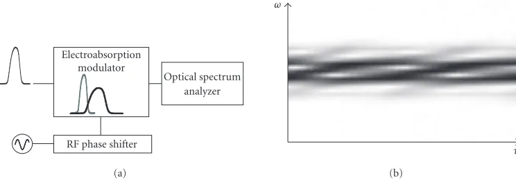
Electroabsorption modulator
Optical spectrum analyzer
RF phase shifter (a)
ω
τ
(b)
Figure5: Example of the implementation of (a) spectrography and (b) spectrogram measured on a 40 GHz alternate-chirp return-to-zero signal with an electroabsorption modulator driven at 10 GHz .
10 8 6 4 2 0
In
te
nsit
y
(a.u.)
−40 −20 0 20 40
Time (ps)
7 6 5 4 3
Phase
(r
ad)
(a)
10 8 6 4 2 0
In
te
nsit
y
(a.u.)
−40 −20 0 20 40
Time (ps)
7 6 5 4 3
Phase
(r
ad)
(b)
Figure6: (a) Intensity and phase of the optical signal (resp., continuous and dashed line). (b) Transmission and phase of the gate (resp., continuous and dashed line) extracted from the previous spectrogram.
experimentally measured spectrogram and from the func-tional form of the spectrogram as the modulus square of the integralE(t)R(t−τ) exp(iωt)dt.
3.2. Experimental spectrography for telecommunication applications
Spectrograms and sonograms are popular tools for ultra-short optical pulse characterization. FROG generates a non-linear spectrogram for the pulse by means of a nonnon-linear op-tical interaction of the pulse under test with one or several of its replicas [22]. This has the experimental advantage of using pump-probe geometries that are commonly used in ultrafast spectroscopy. Adaptations of FROG to pulse characterization in the telecommunication environment can be found, for ex-ample, in [35,36,37,38].
For picosecond pulses, such as those used in telecommu-nications, a gate of smaller bandwidth than needed for fem-tosecond pulses, such as those typically found in ultrafast op-tics applications, suffices. It is possible to implement the gate using a temporal modulator, which has the important ad-vantage of making the entire process linear. It is therefore ex-tremely sensitive to small input pulse energies, yet insensitive to polarization and wavelength [23,39].
The experimental implementation of spectrography with a temporal modulator is straightforward. The pulse under
test is gated by a temporal modulator driven by a control signal synchronized to the pulse under test, as shown in Figure 5a. For example, an electroabsorption modulator can be driven by a sinusoidal voltage with well-defined phase relative to the test pulse. The relative delay τ between the signal under test and the gate is modified by changing the phase of the driving RF sine wave using a voltage-controlled phase shifter. The spectra after the modulator are recorded as a function of the optical frequency ω with a scanning monochromator, or with a Fabry-Perot etalon followed by a photodiode. An example of a measured spectrogram is dis-played inFigure 5b. The characteristics of the pulse train and gate are extracted from the spectrogram, and examples of the retrieved signal and gate when characterizing an alternate-chirp signal [40] are plotted inFigure 6.
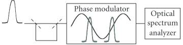
3.3. Interferometry
E(ω)
Linear temporal
phase modulation
E(ω+Ω)
Optical spectrum
analyzer
E(ω) exp(iωτ)
Figure7: Conceptual approach for spectral shearing interferome-try.
single pulse or a coherent pulse train, yieldingNsamples of the field fromαNdata points (α >1). It therefore makes op-timal use of the experimental data.
It is possible to construct the spectral equivalent of spa-tial shearing interferometry, in which the spaspa-tial phase pro-file of a beam is determined by interfering it with a laterally shifted (or sheared) replica. The resulting intensity interfer-ogram can be measured with a square-law detector and the phase simply extracted. The spectral analogue, in which two spectrally sheared pulses are interfered, also allows direct re-construction of the electric field in the spectral domain us-ing the measured spectral phase and a pulse spectrum. Be-cause a single slice of the correlation function is sufficient to characterize the electric field of a pulse that has a continu-ous spectral support, interferometry is viable for most appli-cations. We will focus here on techniques that use the two-time frequency correlation function (or its sampled version)
E(ω)E∗(ω−Ω), whose phaseϕ(ω)−ϕ(ω−Ω) can be con-catenated or integrated to get the spectral phase of the initial pulse [41,42]. For a continuous spectral density, the spectral shearΩis set by the sampling theorem, and it is typically a few percent of the total bandwidth of the pulse under test. Too large a shear would lead to undersampling of the pulse spectrum, while too small a shear could lead to increased sen-sitivity to noise, and thus reduced accuracy of the reconstruc-tion. For a periodic source with high duty cycle, it suffices to measure the intensity and phase of the spectral modes, and the shear can usually be set to the value of the separation be-tween the modes, that is, the repetition rate. The spectral in-tensity can be obtained either from a separate measurement using the spectrometer, or can be extracted from the correla-tion funccorrela-tion directly.
A variety of interferometric techniques are known. The relative phase between adjacent spectral modes can, for ex-ample, be extracted in the time domain after spectral filter-ing [43,44,45,46,47], or in the spectral domain after proper temporal modulation [48]. The latter class of techniques also includes spectral shearing interferometry, where the quantity
E(ω)E∗(ω−Ω) is obtained by measuring the interference of the pulse under test with its sheared replica with an opti-cal spectrum analyzer (Figure 7). The frequency shearΩcan be implemented using a linear temporal phase modulation exp(iΩt). The spectral intensity of the two interfering pulses is|E(ω)|2+|E(ω−Ω)|2+E(ω)E∗(ω−Ω)+E∗(ω)E(ω−Ω). If
a delay is introduced between the nonshifted and the shifted replica, this leads to spectral fringes with small spacing, by virtue of the phaseϕ(ω)−ϕ(ω−Ω) +ωτ. In this case, the interferometric component can be directly extracted using Fourier processing of a single interferogram [49,50].
Phase modulator
Optical spectrum
analyzer
Figure8: Experimental implementation of spectral shearing inter-ferometry.
3.4. Experimental interferometry for telecommunication applications
There are numerous implementations of interferometry for the self-referencing characterization of optical pulses. For spectral shearing interferometry, a spectral shear of arbitrary value can be induced by mixing the test pulse with, for ex-ample, a highly chirped pulse in a nonlinear medium. This is known as spectral phase interferometry for direct electric field reconstruction [49]. A spectral shear can also be in-duced, as explained above, by linear temporal phase mod-ulation of the pulse under test. Such modmod-ulation can be ob-tained using an electro-optic phase modulator driven by an appropriate voltage [50,51]. The generation of a strictly lin-ear voltage at a high frequency is in practice difficult, and it is easier to use a sinusoidal voltage synchronized so that the pulse is at the zero-crossing of the modulation, therefore ex-periencing linear temporal phase modulation. One possible implementation is described inFigure 8.
The pulse under test is split into two replicas. These two replicas, separated by a delayτare sent to a phase modulator driven by a sinusoidal voltage with period 2τ. The synchro-nization is performed so that the two pulses stand at differ-ent zero-crossings of the modulation. Therefore, the pulses are sheared in opposite directions along the frequency axis. IfΩis the shear imposed on one of the pulses, the extracted spectral phase difference isϕ(ω+Ω)−ϕ(ω−Ω) +ωτ. The carrier termωτcan be removed either by turning the mod-ulation off[50] or by measuring a second phase difference when the relative pulse under test and the sine wave driv-ing the modulator has been modified byτ [51]. In this case the extracted spectral phase is ϕ(ω−Ω)−ϕ(ω+Ω) +ωτ; so that the difference between the two extracted phases is 2ϕ(ω+Ω)−2ϕ(ω−Ω).Figure 9displays an experimentally measured interferogram. The rapidly varying fringes due to the delay between the two interfering pulses are evident. An example of the intensity and phase measured using spectral shearing interferometry is also shown.
3.5. Tomography
In
te
nsit
y
(a.u.)
1535 1540 1545 1550
Wavelength (nm)
1541.5 1542
Wavelength (nm) (a)
10 8 6 4 2 0
In
te
nsit
y
(a.u.)
1535 1540 1545 1550
Wavelength (nm)
10 5 0
−5
−10
Phase
(r
ad)
(b)
Figure9: (a) Experimental interferogram and close-up on the fringes. (b) Reconstructed spectral intensity and phase (resp., continuous and dashed line).
inversion algorithm. To see this, notice that a phase-only fil-ter does not provide any information on the frequency or the arrival time of a pulse ensemble and hence, does not consti-tute a measurement of either the spectral or temporal extent of the pulse. So, a tomographic apparatus does not make a simultaneous measurement of the conjugate variables time and frequency. Rather, the quadratic phase modulation acts to rotate the phase space. The square-law detector in com-bination with the amplitude-only filter records the resulting intensity distribution, that is, the projection of the rotated Wigner function. A sufficiently large number of phase-space rotations between−π/2 andπ/2 allows, in principle, recon-struction of the Wigner function via the inverse Radon trans-form [52]. Numerical versions of this inversion algorithm were developed for applications of tomography in areas such as medical imaging, where one aims at reconstructing an ob-ject from a set of its proob-jections (typically, 2D proob-jections of a 3D object, or 1D projections of a 2D object) [53]. A typi-cal implementation of chronocyclic tomography would use a combination of quadratic temporal and spectral phase mod-ulations to rotate the phase space, and optical spectrum mea-surements to project the Wigner function. The Wigner func-tion of the signal under test can be reconstructed from the
measured projections, regardless of the degree of coherence of the pulse ensemble. This capability is unique to tomogra-phy among the techniques presented in this paper. This capa-bility has not been realized experimentally, however, because of the relative difficulty of implementing variable temporal and spectral phase modulations.
The time-to-frequency converter [54,55] operates by ro-tating the Wigner function by π/2, so that a measurement of the frequency marginal after rotation leads to the tem-poral marginal, that is, one obtains the temtem-poral intensity of the signal under test via an optical spectrum measure-ment. However, no phase information is obtained, and this approach requires a large rotation of the Wigner function, which is difficult to obtain.
Phase modulator
Optical spectrum
analyzer
Figure10: Experimental implementation of simplified chronocyclic tomography.
In
te
nsit
y
(a.u.)
−2 −1 0 1 2
Frequency (ps−1)
(a)
10 8 6 4 2 0
In
te
nsit
y
(a.u.)
−2 −1 0 1 2
Frequency (ps−1)
10
5
0
−5
Phase
(r
ad)
(b)
Figure11: (a) Two spectra measured for small positive and negative quadratic temporal phase modulation (continuous and dashed line). (b) Reconstructed spectral intensity and phase (continuous and dashed line).
[56,57]. The fractional power spectrum of the pulse is ob-tained from the rotated Wigner function:
Iα(ω)=
Wtcos(α)+ωsin(α),ωcos(α)−tsin(α)dt. (24)
The derivative of this function with respect to the angle of rotationαatα=0 leads to
∂Iα
∂α = ω ∂W
∂t −t ∂W
∂ω
dt= − ∂
∂ω
tW dt, (25)
and therefore to
∂Iα
∂α = − ∂ ∂ω
I∂ϕ ∂ω
. (26)
A rotation of the phase-space of the pulse requires a com-bination of a quadratic temporal and spectral phase modula-tions. However, the relation in (26) also holds for a shear of the phase-space, in whichωis transformed intoω+ψt, and the temporal coordinate is unchanged. This can be accom-plished by means of a parabolic temporal phase modulation (1/2)ψt2alone. In this case, one finds
∂I0
∂ψ = ∂ ∂ψ
W(ω+ψt,t)dt= ∂
∂ω
I∂ϕ ∂ω
. (27)
This is the form most amenable to experiment, since the bandwidth required to generate a small shear using a phase modulator is modest.
3.6. Experimental chronocyclic tomography
Various implementations of the time-to-frequency converter have been performed using either a phase modulator or non-linear optics. A phase modulator driven by a sinusoidal volt-age can provide quadratic temporal phase modulation to a pulse synchronized with one of its extrema. A nonlinear in-teraction can also provide such modulation.
Simplified chronocyclic tomography has been imple-mented using a temporal phase modulator [57]. The pulse under test was synchronized with a maximum of the phase modulation, and the optical spectrum after modulation mea-sured, as displayed in Figure 10. The pulse under test was then synchronized with a minimum of the phase modula-tion, and the corresponding optical spectrum measured. The derivative ∂I0/∂ψ and the spectrum I(ω) are obtained,
re-spectively, by taking the difference and the sum of the two measured spectra. Equation (26) is then used to reconstruct the phase ϕ(ω).Figure 11displays an experimental pair of measured spectra and the reconstructed intensity and phase for a short optical pulse. The technique can also be improved using synchronous detection of the derivative∂I0/∂ψ, which
enables an increased signal-to-noise ratio [58].
4. CONCLUSION
for pulse-shape characterization, and each may be imple-mented using appropriate linear optical elements. For pulses typical in telecommunications applications, the use of linear temporal modulators as time-nonstationary filters in these classes of measurement has been detailed and experimental implementations for characterization in the telecommunica-tion environment have been presented. As research in both signal analysis and ultrafast optics is in continual develop-ment, it can be expected that further exciting discoveries will be made in the near future.
ACKNOWLEDGMENTS
C. Dorrer would like to acknowledge his fruitful collabora-tion with Inuk Kang, from Bell Laboratories, Lucent Tech-nologies, on the experiments described in [23,39,50,51,57, 58]. I. A. Walmsley acknowledges fruitful interactions with C. Iaconis and M. G. Raymer on methods of wave-field re-construction. The work of I. A. Walmsley was supported by the US National Science Foundation and the UK Engineering and Physical Sciences Research Council.
REFERENCES
[1] I. Kaminow and T. Li,Optical Fiber Telecommunications IV, Academic Press, Boulder, Colo, USA, 2002.
[2] I. A. Walmsley, L. Waxer, and C. Dorrer, “The role of dis-persion in ultrafast optics,”Review of Scientific Instruments, vol. 72, no. 1, pp. 1–29, 2001.
[3] L. Lepetit, G. Cheriaux, and M. Joffre, “Linear techniques of phase measurement by femtosecond spectral interferometry for applications in spectroscopy,”Journal of the Optical Society of America B, vol. 12, no. 12, pp. 2467–2474, 1995.
[4] D. N. Fittinghoff, J. L. Bowie, J. N. Sweetser, et al., “Measure-ment of the intensity and phase of ultraweak, ultrashort laser pulses,”Optics Letters, vol. 21, no. 12, pp. 884–886, 1996. [5] F. K. Fatemi, T. F. Carruthers, and J. W. Lou, “Characterisation
of telecommunications pulse trains by fourier-transform and dual-quadrature spectral interferometry,”Electronics Letters, vol. 39, no. 12, pp. 921–922, 2003.
[6] P. A. Andrekson, “Ultrahigh bandwidth optical sampling os-cilloscopes,” inProc. Optical Fiber Communication Conference (OFC ’04), Los Angeles, Calif, USA, February 2004, Tuo1. [7] C. Dorrer, D. C. Kilper, H. R. Stuart, G. Raybon, and M. G.
Raymer, “Linear optical sampling,”IEEE Photon. Technol. Lett, vol. 15, no. 12, pp. 1746–1748, 2003.
[8] C. Dorrer, J. Leuthold, and C. R. Doerr, “Direct measurement of constellation diagrams of optical sources,” inProc. Opti-cal Fiber Communication Conference (OFC ’04), Los Angeles, Calif, USA, February 2004, PDP33.
[9] I. A. Walmsley and V. Wong, “Characterization of the electric field of ultrashort optical pulses,”Journal of the Optical Society of America B, vol. 13, no. 11, pp. 2453–2463, 1996.
[10] C. Iaconis, V. Wong, and I. A. Walmsley, “Direct interferomet-ric techniques for characterizing ultrashort optical pulses,” IEEE J. Select. Topics Quantum Electron., vol. 4, no. 2, pp. 285– 294, 1998.
[11] J. W. Goodman,Introduction to Fourier Optics, McGraw-Hill, New York, NY, USA, 1996.
[12] S. A. Ponomarenko, G. P. Agrawal, and E. Wolf, “Energy spec-trum of a nonstationary ensemble of pulses,”Optics Letters, vol. 29, no. 4, pp. 394–396, 2004.
[13] M. Born and E. Wolf,Principles of Optics, Cambridge Univer-sity Press, Cambridge, UK, 1998.
[14] K. H. Brenner and J. Ojeda-Castaneda, “Ambiguity function and Wigner distribution function applied to partially coher-ent imagery,”Optica Acta, vol. 31, no. 2, pp. 213–223, 1984. [15] T. A. C. M. Claasen and W. F. G. Mecklenbr¨auker,
“The Wigner distribution—A tool for time-frequency signal analysis—Part III: relations with other time-frequency signal transformations,”Philips Journal of Research, vol. 35, no. 6, pp. 372–389, 1980.
[16] K.-H. Brenner and K. Wodkiewicz, “The time-dependent physical spectrum of light and the wigner distribution func-tion,”Optics Communications, vol. 43, no. 2, pp. 103–106, 1982.
[17] J. Paye, “The chronocyclic representation of ultrashort light pulses,”IEEE J. Quantum Electron., vol. 28, no. 10, pp. 2262– 2273, 1992.
[18] C. A. Hirlimann and J.-F. Morhange, “Wavelet analysis of short light pulses,”Applied Optics, vol. 31, no. 17, pp. 3263– 3266, 1992.
[19] R. Gase, “Time-dependent spectrum of linear optical sys-tems,”Journal of the Optical Society of America A, vol. 8, no. 6, pp. 850–859, 1991.
[20] C. E. Cook and M. Bernfeld,Radar Signals: an Introduction to Theory and Application, Artech House, Norwood, Mass, USA, 1993, incorporated.
[21] L. Cohen,Time-Frequency Analysis, Prentice Hall PTR, Engle-wood Cliffs, NJ, USA, 1995.
[22] R. Trebino, Ed.,Frequency-Resolved Optical Gating: the Mea-surement of Ultrashort Optical Pulses, Kluwer Academic, Boston, Mass, USA , 2002.
[23] C. Dorrer and I. Kang, “Simultaneous temporal characteriza-tion of telecommunicacharacteriza-tion optical pulses and modulators by use of spectrograms,”Optics Letters, vol. 27, no. 15, pp. 1315– 1317, 2002.
[24] V. Wong and I. A. Walmsley, “Ultrashort-pulse characteriza-tion from dynamic spectrograms by iterative phase retrieval,” Journal of the Optical Society of America B, vol. 14, no. 4, pp. 944–949, 1997.
[25] D. T. Reid, “Algorithm for complete and rapid retrieval of ul-trashort pulse amplitude and phase from a sonogram,”IEEE J. Quantum Electron., vol. 35, no. 11, pp. 1584–1589, 1999. [26] V. Wong and I. A. Walmsley, “Phase retrieval in time-resolved
spectral phase measurement”, in Generation, Amplification, and Measurement of Ultrashort Laser Pulses II, vol. 2377 of Proceedings of SPIE, pp. 178–186, San Jose, Calif, USA, April 1995.
[27] K. Kikuchi, “Theory of sonogram characterization of optical pulses,”IEEE J. Quantum Electron., vol. 37, no. 4, pp. 533–537, 2001.
[28] E. B. Treacy, “Measurement and interpretation of dynamic spectrograms of picosecond light pulses,”Journal of Applied Physics, vol. 42, no. 10, pp. 3848–3858, 1971.
[29] J. L. A. Chilla and O. E. Martinez, “Analysis of a method of phase measurement of ultrashort pulses in the frequency do-main,”IEEE J. Quantum Electron., vol. 27, no. 5, pp. 1228– 1235, 1991.
[30] K. Mori, T. Morioka, and M. Saruwatari, “Group velocity dispersion measurement using supercontinuum picosecond pulses generated in an optical fibre,”Electronics Letters, vol. 29, no. 11, pp. 987–989, 1993.
[32] H. Stark, Ed.,Image Recovery: Theory and Application, Aca-demic Press, New York, NY, USA, 1987.
[33] D. J. Kane, G. Rodriguez, A. J. Taylor, and T. S. Clement, “Si-multaneous measurement of two ultrashort laser pulses from a single spectrogram in a single shot,”Journal of the Optical Society of America B, vol. 14, no. 4, pp. 935–943, 1997. [34] D. J. Kane, “Real-time measurement of ultrashort laser pulses
using principal component generalized projections,”IEEE J. Select. Topics Quantum Electron., vol. 4, no. 2, pp. 278–284, 1998.
[35] M. D. Thomson, J. M. Dudley, L. P. Barry, and J. D. Harvey, “Completepulse characterization at 1.5µm by cross-phase modulation in optical fibers,”Optics Letters, vol. 23, no. 20, pp. 1582–1584, 1998.
[36] K. Ogawa and M. D. Pelusi, “High-sensitivity pulse spectro-gram measurement using two-photon absorption in a semi-conductor at 1.5-µm wavelength,”Optics Express, vol. 7, no. 3, pp. 135–140, 2000.
[37] P.-A. Lacourt, J. M. Dudley, M. Merolla, H. Porte, J.-P. Goedgebuer, and W. T. Rhodes, “Milliwatt-peak-power pulse characterization at 1.55µm by wavelength-conversion frequency-resolved optical gating,” Optics Letters, vol. 27, no. 10, pp. 863–865, 2002.
[38] L. P. Barry, S. Del Burgo, B. Thomsen, R. T. Watts, D. A. Reid, and J. Harvey, “Optimization of optical data transmitters for 40 Gb/s lightwave systems using frequency resolved optical gating,”IEEE Photon. Technol. Lett., vol. 14, no. 7, pp. 971– 973, 2002.
[39] C. Dorrer and I. Kang, “Real-time implementation of linear spectrograms for the characterization of high bit-rate opti-cal pulse trains,”IEEE Photon. Technol. Lett., vol. 16, no. 3, pp. 858–860, 2004.
[40] P. J. Winzer, C. Dorrer, R.-J. Essiambre, and I. Kang, “Chirped return-to-zero modulation by imbalanced pulse carver driv-ing signals,” IEEE Photon. Technol. Lett., vol. 16, no. 5, pp. 1379–1381, 2004.
[41] V. A. Zubov and T. I. Kuznetsova, “Solution of the phase prob-lem for time-dependent optical signals by an interference sys-tem,”Soviet Journal of Quantum Electronics, vol. 21, pp. 1285– 1286, 1991.
[42] V. Wong and I. A. Walmsley, “Analysis of ultrashort pulse-shape measurement using linear interferometers,”Optics Let-ters, vol. 19, no. 4, pp. 287–289, 1994.
[43] K. C. Chu, J. P. Heritage, R. S. Grant, et al., “Direct measure-ment of the spectral phase of femtosecond pulses,”Optics Let-ters, vol. 20, no. 8, pp. 904–906, 1995.
[44] P. Kockaert, M. Peeters, S. Coen, Ph. Emplit, M. Haelter-man, and O. Deparis, “Simple amplitude and phase measur-ing technique for ultrahigh-repetition-rate lasers,”IEEE Pho-ton. Technol. Lett, vol. 12, no. 2, pp. 187–189, 2000.
[45] M. Kwakernaak, R. Schreieck, A. Neiger, H. Jackel, E. Gini, and W. Vogt, “Spectral phase measurement of mode-locked diode laser pulses by beating sidebands generated by elec-trooptical mixing,”IEEE Photon. Technol. Lett., vol. 12, no. 12, pp. 1677–1679, 2000.
[46] P. Kockaert, J. Azana, L. R. Chen, and S. LaRochelle, “Full characterization of uniform ultrahigh-speed trains of optical pulses using fiber Bragg gratings and linear detectors,”IEEE Photon. Technol. Lett., vol. 16, no. 6, pp. 1540–1542, 2004. [47] P. Kockaert, M. Haelterman, Ph. Emplit, and C. Froehly,
“Complete characterization of (ultra)short optical pulses us-ing fast linear detectors,”IEEE J. Select. Topics Quantum Elec-tron., vol. 10, no. 1, pp. 206–212, 2004.
[48] J. Debeau, B. Kowalski, and R. Boittin, “Simple method for the complete characterization of an optical pulse,”Optics Letters, vol. 23, no. 22, pp. 1784–1786, 1998.
[49] C. Iaconis and I. A. Walmsley, “Spectral phase interferome-try for direct electric-field reconstruction of ultrashort optical pulses,”Optics Letters, vol. 23, no. 10, pp. 792–794, 1998. [50] C. Dorrer and I. Kang, “Highly sensitive direct
characteriza-tion of femtosecond pulses by electro-optic spectral shearing interferometry,”Optics Letters, vol. 28, no. 6, pp. 477–479, 2003.
[51] I. Kang, C. Dorrer, and F. Quochi, “Implementation of electro-optic spectral shearing interferometry for ultra-short pulse characterization,”Optics Letters, vol. 28, no. 22, pp. 2264–2266, 2003.
[52] M. Beck, M. G. Raymer, I. A. Walmsley, and V. Wong, “Chronocyclic tomography for measuring the amplitude and phase structure of optical pulses,” Optics Letters, vol. 18, no. 23, pp. 2041–2043, 1993.
[53] A. C. Kak and M. Slaney,Principles of Computerized Tomo-graphic Imaging, IEEE Press, New York, NY, USA, 1988. [54] M. T. Kauffman, W. C. Banyai, A. A. Godil, and D. M. Bloom,
“Time-to-frequency converter for measuring picosecond op-tical pulses,”Applied Physics Letters, vol. 64, no. 3, pp. 270– 272, 1994.
[55] L. Kh. Mouradian, F. Louradour, V. Messager, A. Barth´el´emy, and C. Froehly, “Spectro-temporal imaging of femtosecond events,”IEEE J. Quantum Electron., vol. 36, no. 7, pp. 795– 801, 2000.
[56] T. Alieva, M. J. Bastiaans, and L. Stankovic, “Signal recon-struction from two close fractional Fourier power spectra,” IEEE Trans. Signal Processing, vol. 51, no. 1, pp. 112–123, 2003. [57] C. Dorrer and I. Kang, “Complete temporal characterization of short optical pulses by simplified chronocyclic tomogra-phy,”Optics Letters, vol. 28, no. 16, pp. 1481–1483, 2003. [58] I. Kang and C. Dorrer, “Highly sensitive differential
tomo-graphic technique for real-time ultrashort pulse characteriza-tion,” inProc. Conference on Lasers and Electro-Optics (CLEO ’04), vol. 1, San Francisco, Calif, USA, May 2004, CTuZ6.
Christophe Dorreris a Member of
Techni-cal Staffat Bell Laboratories, Lucent Tech-nologies. He has a Ph.D. degree in op-tics from the ´Ecole Polytechnique, France. He works in various domains of ultrafast optics related to optical telecommunica-tions, such as optical pulse characteriza-tion, characterization of high-bit-rate data-encoded sources, characterization of de-vices and fibers, pulse shaping, and moni-toring of optical networks.
Ian A. Walmsleyis the Hook Professor of
expermental physics at the University of Oxford, and the Head of the Department of Atomic and Laser Physics, Clarendon Lab-oratory. He has a Ph.D. degree in optics from the University of Rochester. His re-search concerns quantum processes on ul-trafast time scales, and he has developed methods for the generation and measure-ment of nonclassical states of light and