Instantaneous Frequency Estimation Using
Stochastic Calculus and Bootstrapping
A. Abutaleb
Systems and Bioengineering Department, School of Engineering, Cairo University, 12613 Giza, Egypt Email:[email protected]
Received 15 July 2004; Revised 6 March 2005; Recommended for Publication by Frank Ehlers
Stochastic calculus methods are used to estimate the instantaneous frequency of a signal. The frequency is modeled as a polynomial in time. It is assumed that the phase has a Brownian-motion component. Using stochastic calculus, one is able to develop a stochastic differential equation that relates the observations to instantaneous frequency. Pseudo-maximum likelihood estimates are obtained through Girsanov theory and the Radon-Nikodym derivative. Bootstrapping is used to find the bias and the confidence interval of the estimates of the instantaneous frequency. An approximate expression for the Cram´er-Rao lower bound is derived. An example is given, and a comparison to existing methods is provided.
Keywords and phrases:bootstrapping, Ito calculus, instantaneous frequency, time-varying frequency, Girsanov theory.
1. INTRODUCTION
Over the past several years there has been a marked increase in the application of coherent signal and image processing. Coherent processing requires an accurate estimate of the phase (Blackledge [1]). Examples where coherent process-ing is required include synthetic aperture radar (SAR), syn-thetic aperture sonar, adaptive beam forming, acoustic imag-ing, projection and diffraction tomography, adaptive optics, magnetic resonance imaging (MRI), and inverse synthetic aperture radar (ISAR) (see Goldstein et al. [2], Song et al. [3], Ghiglia and Pritt [4]). Phase estimation also has many applications in the areas of radar (Wehner [5]) and commu-nications (Li [6]) and others. The instantaneous frequency (IF) is defined as the derivative of the phase.
There are mainly two approaches for the estimation of the IF of the time-varying frequency signals; parametric and nonparametric (Chen and Ling [7]). In the nonparametric approach, if the signal has frequency contents that are rapidly changing over time, one of the most popular approaches is to use short-time Fourier transform (STFT). In this approach, the signal is divided into overlapping segments. The fast Fourier transform (FFT) is then applied to each segment. By observing the evolution of the frequency components over time, one should be able to estimate both the frequency com-ponents and their magnitudes (Wehner [5]). This approach suffers from the poor resolution of the FFT, and the large amount of needed data to get reasonable results. Neverthe-less, the STFT gives us some idea about the complexity of the data and suggests probable models for the IF.
The Wigner-Ville distribution has proven to be the most suitable nonparametric approach to handle instantaneous frequency estimation (IEEE [8]). Several modifications have been suggested, that concentrate on the choice of the window (see Katkovnik and Stankovic [9], Barkat [10]). Still, a major requirement of the Wigner-Ville distribution is the large size of the data, a situation that is not available in some applica-tions.
In the parametric approach, the phase is modeled as an autoregressive (AR) process, moving average (MA) process, or a polynomial (Benidir and Ouldali [11]). The coefficients of the model are estimated adaptively using the least mean square algorithm (LMS), the recursive least square (RLS) al-gorithm, phase-locked loop (PLL), or others such as hidden Markov models (see Goto et al. [12], IEEE [8]). For large data sizes, however, the accuracy of the parametric methods was shown to be less than the nonparametric methods. Obviously if the parametric model is accurate, then it should outper-form any nonparametric method. The parametric methods on the other hand work better for small-size data (Boashash [13]).
algorithm was introduced to estimate the polynomial phase (Golden and Friedlander [17]). The major problems with these two algorithms are the required large number of data, and the needed, relatively, high SNR (30 dB and above) to obtain good estimates.
In this paper, we introduce a new parametric approach that is based on the stochastic (Ito) calculus. Concepts from stochastic or Ito calculus (Kloeden and Platen [18]) are used to set up the phase estimation problem. Assuming that the phase could be modeled as a polynomial in time with a scaled additive Brownian motion, which is a common model for random media transmission, one could develop a stochas-tic differential equation (SDE) for the observations. Other models for the phase or the amplitude could be tackled with the same approach. For this model of the phase, the SDE is a linear equation in the unknown coefficients of the polyno-mial phase but nonlinear in the other parameters. This way a nonlinear estimation problem has been transformed into a partially linear estimation problem. Using the Girsanov the-ory, and assuming complete knowledge of the other param-eters of the signal, one is able to find an exact expression for the likelihood function of the observations. This is actu-ally a likelihood function. Maximizing this pseudo-likelihood function with respect to the unknown coefficients of the phase, one is able to find a closed form solution for these coefficients. Simulation-based methods (McFadden [19]) are used to estimate the other parameters of the signal. Moreover, approximate statistical properties of the pseudo-maximum likelihood estimates of the coefficients of the phase were obtained in a straightforward fashion. Ap-proximate expressions for the Cram´er-Rao lower bounds for the variances of the estimates were easily obtained; an-other advantage of using Ito calculus. While many estima-tion problems could be cast in a discrete time setting, there is no equivalent in the discrete time to Ito’s lemma; a fun-damental result in stochastic calculus. Thus, one has to use continuous time models in order to take advantage of the Ito calculus properties. “It should be added that in some cases it is easier, at first, to study the continuous analog of problems formulated for discrete time, and use the results obtained in the solution of the latter” (Lipster and Shiryayev [20, Volume I]). In some cases, however, using stochastic calculus would be cumbersome and the discrete methods of time series anal-ysis would be much easier to use.
In the given examples, the required SNR to get good esti-mates of the phase is more than 10 dB. Using the bootstrap-ping method, one was able to obtain good results at lower SNR. Bootstrap is a method that handles small samples and yields good estimates for the bias and the confidence intervals for the estimates (see Efron and Tibshirani [21], Zaman [22], Politis [23], Zoubir and Boashash [24]). It was not meant to be a method to improve the accuracy of the estimates. Using the peak of the histogram, generated from the boot-strapping method for each estimated parameter, as the de-sired estimate of the unknown parameter, one is able to get good estimates at lower SNR. This was observed in this report and in some other applications (see Souza and Neto [25], Abutaleb [26]). Through the bootstrapping method, one is
able to generate a large number of samples from the mea-sured small sample data. Bootstrapping amounts to treating the observed samples as if they exactly represent the whole population. In nonparametric bootstrapping, drawing from this sample space, at random with replacement, will generate as many samples as desired. In parametric bootstrapping, a model is used to generate as many samples as desired. The bootstrapping method found many applications in the area of statistical signal processing (Zoubir and Boashash [24]).
This paper is divided as follows:Section 2describes the mathematical formulation of the phase estimation prob-lem and an approximate maximum likelihood method is described. We also describe in this section the method of stochastic annealing. In Section 3, the proposed stochastic-calculus-based approach is introduced and the statistical properties of the estimates are given. A discussion of the bootstrapping method is also given. InSection 4, we present simulation results and comparison to the approximate maxi-mum likelihood method ofSection 2. InSection 5, summary and conclusions are given.
2. PROBLEM FORMULATION
The real signal, z(t), with one phase component could be modeled as follows:
z(t)=A(t) sinφ(t)+ε(t), (1)
where
φ(t)=2π
I
i=1
fiti+γB(t), (2)
I is the order of the polynomial,A(t) is the amplitude,φ(t) is the phase, B(t) is a Brownian motion,γis an unknown constant, andε(t) is an additive white noise process of
un-known variance σ2. The one phase component could
rep-resent the radar tracking of just one target, that is, maneu-vering. It could also represent the tracking of one target in a sequence of images.
For constant phase component and polynomial fre-quency we have
φ(t)=2π
I
i=0
fiti+γB(t). (3)
In this paper we will be concerned with the situation whereA(t)=1, and the error/noise termε(t) is imbedded in the random part of the phase, that is, we are interested in the model
z(t)=sinφ(t). (4)
such as the Ornstein-Uhlenbeck process, and other models for the amplitude could also be tackled with the proposed stochastic-calculus-based approach. This will be the subject of other reports (Abutaleb [27]). The case where we have more than one stochastic IF is currently under investigation using what is called the Malliavin calculus (see Abutaleb and Papaioannou [28], Nualart [29]).
2.1. Approximate maximum likelihood method
To estimate the unknown coefficients, fi, one could ignore
the Brownian motion term, γB(t), and use nonlinear least square methods (Goto et al. [12]), the genetic algorithms (Abutaleb [30]), or stochastic annealing (Kloeden and Platen [18]). Specifically, in the least square approach, the instanta-neous phaseφLS(t) is assumed to be pure polynomial in the frequency, that is,
z(t)=sinφLS(t)+ε(t), (5)
where
φLS(t)=2π
I
i=1
fiti. (6)
One could then find the unknowns by minimizing the sum of squared error,{z(t)−sin[φLS(t)]}2. While this approach is approximate, it gives an indication about the estimates of the unknown parameters that could be used later on to guide the search area with numerical methods. The above approach is a simplification to the true problem since the correct expres-sion should be
z(t)=sinφ(t)=sinφLS(t)cosγB(t)
+ cosφLS(t)sinγB(t), (7)
and whenγ→0, we get the approximate expression
z(t)=sinφ(t)≈sinφLS(t)+ cosφLS(t)γB(t), (8)
that is,
z(t)≈sinφLS(t)+ε(t), (9)
whereε(t)≈cos[φLS(t)][γB(t)], that is, the error is function of the unknown parameters.
In discrete time, one could write (8) as
z(k)=sinφ(k)≈sinφLS(k)+cosφLS(k)
γ√∆
k
j=0
w(j)
,
(10)
whereφLS(k)=2πIi=1fi(k∆)i,B(t)=
√
∆k
j=0w(j),∆is the sampling interval, andw(j) is Gaussian with zero mean and variance 1.
Rearranging (10) we get
z(k)−sinφLS(k)
γ√∆cosφLS(k) ≈
k
j=0
w(j)
, (11)
and for time (k+ 1) we get
z(k+ 1)−sinφLS(k+ 1)
γ√∆cosφLS(k+ 1) ≈
k+1
j=0
w(j)
. (12)
Subtracting the expressions atkand at (k+ 1) we get
−
z(k)−sinφLS(k)
γ√∆cosφLS(k) +
z(k+ 1)−sinφLS(k+ 1)
γ√∆cosφLS(k+ 1)
≈w(k+ 1).
(13)
Rearranging (13) we get
z(k+ 1)=sinφLS(k+ 1)
+
z(k)−sinφLS(k)
γ√∆cosφLS(k)
γ√∆cosφLS(k+ 1)
+γ√∆cosφLS(k+ 1)w(k+ 1).
(14)
The conditional probability density function (pdf) f[z(k+ 1)|z(k)] is thus given by
fz(k+ 1)|z(k)
=exp−(1/2)
z(k+1)−sinφLS(k+1)−z(k)−sinφLS(k)/γ√∆cosφLS(k)γ√∆cosφLS(k+1)2/γ2∆cos2φLS(k+1)
2πγ2∆cos2φLS(k+ 1) .
The likelihood function, which is the joint pdf of the obser-vations, is thus given by
fz(N),z(N−1),. . .,z(1)= fz(1)
N−1
k=1
fz(k+ 1)|z(k),
(16)
and the log likelihood functionλ, ignoring the initial
condi-tions, is given by
λ=logfz(N),z(N−1),. . .,z(1)
=
N−1
k=1
logfz(k+ 1)|z(k).
(17)
Substituting for the expression in (15) into (17), we get
λ=logfz(N),z(N−1),. . .
= −1 2
N−1
k=1
log2πγ2∆cos2φLS(k+ 1)
−1 2
N−1
k=1
z(k+ 1)−sinφLS(k+ 1)−z(k)−sinφLS(k)/γ√∆cosφLS(k)γ√∆cosφLS(k+ 1)2
γ2∆cos2φLS(k+ 1) .
(18)
Maximizing the log likelihood function of (18) with respect to the unknown coefficients, fiandγ, yields the desired
esti-mates.
Due to the nonlinearities in the log likelihood function, one would expect the existence of several local minima and we should use global optimization methods. Thus, it is pro-posed that the frequencies and γbe estimated through the stochastic annealing method, which is known to have good numerical properties. Other methods such as genetic algo-rithms could also be used.
2.2. Parameter estimation through stochastic annealing
In the stochastic annealing method, for each unknown pa-rameter we develop a stochastic equation. The solution of which is the maximum likelihood estimate of the parameter. This is explained in what is to follow.
The stochastic differential equation (SDE) of the un-known parameters is given by
df(t)= −∇λ f(t),γ(t)+σ(t)dBf(t) (19)
which has the discrete form
f(k+ 1)=f(k)− ∇λ f(k),γ(k)+σ(k)∆Bf(k), (20)
whereBf(t) is a vector Brownian motion,∆Bf(k) is a
vec-tor white Gaussian noise. Each element has zero mean and variance∆,∆is the sampling interval.∇λ(f(k),γ(k)) is the gradient ofλ(f,γ) with respect to f.
A similar equation forγis used:
dγ(t)= −∇λ f(t),γ(t)+σ(t)dBγ(t), (21)
where Bγ(t) is Brownian motion, and∇λ[f(t),γ(t)] is the
gradient ofλ(f,γ) with respect toγ, and is defined as
∇λγ(k)=λ f(k),γ(k)
−λ f(k),γ(k−1)
γ(k)−γ(k−1) . (22)
The variance is defined as
σ(t)= c
log(t+ 2), c >0. (23)
The choice above forσ(t) is shown to give quick convergence (Kloeden and Platen [18]). Other choices forσ(t) are also possible.
2.3. The Wigner-Ville distribution
The most common nonparametric method to estimate the instantaneous frequency is through the Wigner-Ville distri-bution (WVD) and its modifications. The WVD(t,ω) at in-stanttand frequencyωof a signalz(t) and its complex con-jugatez∗(t) is defined as (Chen and Ling [7])
WVD(t,ω)=
dtz
t+t
2
z∗
t−t
2
exp(−jωt) (24)
which has the discrete form (Boashash [13])
WVD(n,k)=
M
m=−M
z
n+m
2
z∗
n−m
2
exp
−j2πmk M
,
(25)
For a sampling interval∆, the discrete WVD is given as (Boashash and Black [31])
WVD(n∆,f)
=2∆
M
m=−M
z(nT+m∆)z∗(n−m∆) exp(−j4π f m∆),
(26)
whereM=(N−1)/2, andNis the number of data points. Both formulae (25) and (26) are used in the literature.
The instantaneous frequency f(n) derived via the first moment of the discrete WVD is given by
f(n)= M
2π
M−1
k=0
WVD(n,k) exp
j2π k
M
mod 2π. (27)
InSection 4, the instantaneous frequency of (27) is com-pared to the true values. It is shown that they are far apart. Thus, the WVD approach was not used for further compar-isons.
2.4. The Hilbert transform and the analytic function
A given real signalz(t) can be used to construct a complex waveform,za(t), as
za(t)=
1 √ 2
z(t) +jz(t), (28)
where z(t) is the Hilbert transform of z(t) and is given as (Cohen [32])
z(t)= 1
π
∞
−∞
z(τ)
t−τdτ. (29)
The complex waveform,za(t), is the analytic representation
ofz(t) and could be calculated either in the time domain us-ing a finite impulse response (FIR) filter or in the frequency domain as follows (Boashash [33]).
(1) Take theN-point discrete Fourier transform ofz(n) to get DFT[z(n)],n=0,. . .,N−1.
(2) Define
DFTza(k)
=
DFTz(k), k=0,N 2,
2 DFTz(k), k=1,. . .,N 2 −1,
0, k=N
2 + 1,. . .,N−1.
(30)
(3) Calculateza(n)=IDFT{DFT[za(k)]},n=0,. . .,N−
1, where IDFT is the inverse Fourier transform.
The phase angle is then calculated and fitted to the as-sumed model of the phase. The phase angle,φAnalytic, is de-fined as
φAnalytic=arctan
Imaginaryza(t)
Realza(t)
. (31)
InSection 4, the analytic phase,φAnalyticof (31), is esti-mated and compared to the true value. It is shown that they are far apart. Thus, the analytic signal approach was not used.
3. ITO CALCULUS FOR PHASE ESTIMATION: THE PROPOSED APPROACH
In this section, we introduce the stochastic-calculus-based approach for phase estimation. It is assumed that the ran-domness in the signal is due to the Brownian-motion com-ponent in the phase. Other models of the signal could also be treated in the same way.
3.1. Derivation of the SDE for the observation
As inSection 2, the received signal is modeled as
z(t)=sin
2π
I
i=1
fiti+γB(t)
, (32)
where it is assumed that the additive error is imbedded in the random component (Wiener process or Brownian motion)
B(t).
Letx(t)=B(t), thus
dx(t)=dB(t), (33)
wheredx(t) is the stochastic differential forx(t), anddB(t) is what is known as white Gaussian noise with zero mean and variancedt. We need to find a stochastic differential equation (SDE) fordz(t). In order to do that, we first introduce the general form for SDE and for nonlinear transformation.
The general form for a stochastic differential equation is
dx(t)=at,x(t)dt+bt,x(t)dB(t). (34)
In our case, (33),a(t,x(t))=0, andb(t,x(t))=1.
LetU1(t,x(t)) be a nonlinear transformation ofx(t), that is,z(t)=U1(t,x(t)), using Ito lemma (Kloeden and Platen [18]) we obtain
dz(t)=
∂U1
∂t +a
t,x(t)∂U1
∂x +
1 2b
2t,x(t)∂2U1
∂x2
dt
+bt,x(t)∂U1
∂x dB(t).
In our case,
z(t)=U1t,x(t)=sin
2π
I
i=1
fiti+γx(t)
, (36)
x(t)=B(t), at,x(t)=0, bt,x(t)=1,
∂U1
∂t =2π
I−1
i=1
iti−1f
i
cos
2π
I
i=1
fiti+γx(t)
,
∂U1
∂x =γcos
2π
I
i=1
fiti+γx(t)
,
∂2U1
∂x2 = −γ
2sin
2π
I
i=1
fiti+γx(t)
.
(37)
Substituting the expressions of (37) into (35) we get
dz(t)=
2π
I
i=1
iti−1f
i
1−z2(t)−1 2γ
2z(t)
dt
+γ1−z2(t)dB(t),
(38)
where we chose cosx =(1−sin2x). Nevertheless, one has to choose the right sign of the cos(x) depending on which quadrant liesx.
Let
f =f1 f2 · · · fI T
, (39)
and let
a(t)=2π1 2t · · · ItI−1 T. (40) Then (38) could be written compactly as
dz(t)=
!
aT(t)f1−z2(t)−1
2γ
2z(t)
" dt
+γ1−z2(t)dB(t).
(41)
The stochastic processz(t) has the following SDE form:
dz(t)=ct,z(t)dt+et,z(t)dB(t), (42)
where
ct,z(t)=
!
aT(t)f1−z2(t)−1
2γ
2z(t)
"
,
et,z(t)=γ1−z2(t).
(43)
Notice that the SDE ofz(t) turned out to be linear in the un-known frequency components, f. This is one advantage of using Ito calculus. Other forms of the phase may not yield this nice linear property however. One could stop here and derive an approximate expression for the likelihood func-tion of the observafunc-tions as we did inSection 2. Instead we go through the rigorous derivation of the exact likelihood func-tion.
3.2. Pseudo-maximum likelihood estimation
3.2.1. The pseudo-maximum likelihood estimates of the unknown parameters
Let the unknown parameters be defined as the vectorθ =
[fTγ]T, and then the SDE of the observations, dz(t), is
rewritten as
dz(t)=ct,z(t);θdt+et,z(t);γdB(t). (44)
According to the Girsanov theory and for a known γ, the Radon-Nikodym derivative which is the likelihood function, L, is given by (see Lipster and Shiryayev [20], Oksendal [34], Prakasa Rao [35])
Lt,z(t);θ
=exp
−1 2
t
0
c2s,z(s);θds
e2s,z(s);γ +
t
0
cs,z(s);θdz(s)
e2s,z(s);γ
,
(45)
and the log likelihood functionλ=lnLbecomes
λ=lnLt,z(t);θ
=−1 2
t
0
c2s,z(s);θds
e2s,z(s);γ +
t
0
cs,z(s);θdz(s)
e2s,z(s);γ .
(46)
Substituting the expressions for c[t,z(t);θ] and e[t,z(t);γ] into (46), we get the log likelihood function as
λ=lnLt,z(t);θ
=−1 2
t
0 #
aT(s)f1−z2(s)−(1/2)γ2z(s)$2ds
γ21−z2(s)
+
t
0 #
aT(s)f1−z2(s)−(1/2)γ2z(s)$dz(s)
γ21−z2(s) .
(47)
Equation (45) is a true likelihood function as long asγ is known. And sinceγwill be replaced by its estimateγ, (45) represents a pseudo-likelihood function. Maximizing the log of the pseudo-likelihood functionλ = lnLwith respect to the unknown vector f and assuming estimateγ, one could get the pseudo-maximum likelihood estimate of f as follows:
∂λ
∂ f =0
=−
t
0 #
1−z2(s)a(s)$#aT(s)f1−z2(s)−(1/2)γ2z(s)$ds
γ21−z2(s)
+
t
0 #
1−z2(s)a(s)$dz(s)
γ21−z2(s) .
This is reduced to
1
γ2
! t
0a(s)a
T(s)ds
" f
=
t
0
a(s)dz(s)
γ21−z2(s) +
1 2
t
0
a(s)z(s)ds
1−z2(s) . (49)
Finally the pseudo-maximum likelihood estimate of f is
given as
f =
! t
0a(s)a
T(s)ds
"−1t
0
a(s)dz(s)
1−z2(s)
+γ 2
2
! t
0a(s)a
T(s)ds
"−1t
0
a(s)z(s)ds
1−z2(s) .
(50a)
Substituting fordz(s) in (50) we get
f = f +
γ
t
0a(s)dB(s)
! t
0a(s)a
T(s)ds
"−1. (50b)
To estimate the unknown parameterγ, one has to go through another route. This is explained inSection 3.2.3.
3.2.2. Another derivation for the pseudo-maximum likelihood estimates
In the previous subsection, the pseudo-maximum likelihood estimates were obtained using the observed data sequence, z(t). If one is able to find an initial guess forγ, using, for ex-ample, the approximated method ofSection 2, one could ap-ply a transformation to the data and derive an easier method to find the pseudo-maximum likelihood estimate of the vec-tor f. This approach, however, is tricky. It is always better to work with the original data. The simulations showed the ac-curacy of the approach presented inSection 2.2compared to the one presented here. We present the derivation any way because we will need some of its results when calculating the Cram´er-Rao lower bound.
To find the pseudo-maximum likelihood estimates of the unknown parameters, it will be easier if the coefficient of the Brownian motion is unity. Thus, we need to find another transformationy(t)=U2(t,z(t)) such that
d y(t)=gt,y(t)dt+dB(t). (51)
We pickU2(t,z(t)) such that
∂U2
∂z =
1
et,z(t) =
1
γ1−z2(t)=
1 γ
1−z2(t)−1/2,
∂U2
∂t =0,
(52)
and thus,
∂2U2
∂z2 =
1
γz(t)
1−z2(t)−3/2
. (53)
Integrating∂U2/∂zwith respect toz(t) we get
y(t)=U2t,z(t)= 1
γsin
−1z(t), (54)
that is,
z(t)=sinγy(t), (55)
where we have chosen to set the constant of integration to zero.
The expression forg(t,y(t)) is given as follows:
gt,y(t)|z(t)=sin(γy(t))=∂U2
∂t +c
t,z(t)∂U2
∂z
+1
2e
2t,z(t)∂2U2
∂z2 .
(56)
Substituting (52) and (53) into (56) we get
gt,z(t)
=
!
aT(t)f1−z2(t)−1
2γ
2z(t)
"
1 γ
1−z2(t)−1/2
+1
2γ
21−z2(t)
1
γz(t)
1−z2(t)−3/2
(57)
which is reduced to
gt,z(t)= 1
γ
aT(t)f. (58)
Substituting (58) into (51), we get the SDE ford y(t) as fol-lows:
d y(t)=1
γ
aT(t)fdt+dB(t). (59)
This form ofd y(t) has the coefficients ofdB(t) unity. This will make the derivation of the Cram´er-Rao lower bound easier and tractable (Oksendal [34]). Remember that f = [f1 f2 · · · fI]Tanda(t)=2π[1 2t · · · ItI−1]T.
According to the Girsanov theory and for a givenγ, the Radon-Nikodym derivative, which is the pseudo-likelihood function,L, is given by (Oksendal [34])
L=exp
−21
t
0
1
γa
T(s)f
2
ds+
t
0
1
γa
T(s)f
d y(s)
,
and the log of the pseudo-likelihood function λ = logLis given as
λ=logL= −1
2
t
0
1
γa
T(s)f
2
ds+
t
0
1
γa
T(s)f
d y(s).
(61)
Maximizing the log of the pseudo-likelihood function λ = logL with respect to the unknowns f, one could get the pseudo-maximum likelihood estimate of the unknowns. Re-member that in this expression, however, we use the sequence of transformed datay(t), not the observed dataz(t). Thus, an initial guess forγmust be available.
3.2.3. Simulation-based estimation ofγ
Equation (45) is a true likelihood function as long as the dif-fusion term, e(t,z(t);γ), is completely known, that is,γ is known. In practice, we do not know γ. As a matter of fact it is one of the unknowns that we need to estimate. There are many methods to estimateγ. A popular, yet not accurate, method to estimateγ(Yoshida [36]) is through the observa-tion that
dz(t)2=γ21−z2(t)dt. (62)
One could use this equation or its modifications to find an estimate forγ. Instead we use the more accurate simulation-based method of McFadden [19] to find γ. The following steps describe the algorithm. (1) For a given estimate f, we simulate a sequence of data points through (4) and we cal-culate the sum of the squared differences between the sim-ulated and the observed data; this is the error criterion. (2) We change γ; using the method of stochastic annealing of
Section 2.2, till the sum of squared error is minimized. (3) Use the maximum likelihood method ofSection 3.1with the estimatedγto find a new estimate for f. (4) Go to step (1). (5) Stop when there is no more reduction in the sum of the squared error. Specifically for an estimated f, and for a given
γ, simulate the phaseφ(t) given by
φ(t)=2π
I
i=0
fiti+γB(t). (63)
Thus, the simulated signalz(t) is given by
z(t)=sin φ(t). (64)
The error criterion is defined as
optimization criterion forγ=
t
z(t)−z(t)2. (65)
3.2.4. Pseudo-maximum likelihood estimate forf
The pseudo-maximum likelihood estimates of the coeffi
-cients of the polynomial phase are obtained as
λ=logL=−1
2
t
0
1
γa
T(s)f
2
ds+
t
0
1
γa
T(s)f
d y(s),
∂λ
∂ f|γ=γ,f=f=0=−
t
0 1
γa(s)
1
γa
T(s)f
ds+1
γ t
0a(s)d y(s).
(66)
Rearranging we get
t
0a(s)a
T(s)ds
f =γ
t
0a(s)d y(s), (67)
that is,
f =γ
t
0a(s)a
T(s)ds
−1t
0a(s)d y(s) (68)
which is a closed form solution for estimates of the coef-ficients of the polynomial phase. Remember that a(t) = 2π[1 (2t) · · · (ItI−1)]T,z(t) = sin[γy(t)], and it is z(t)
that we observe. Thus, in (68) we substitute for y(t) = {sin−1[z(t)]}/γ.
While (68) seems to be easier to evaluate than (50), we recommend not using it due to the discontinuities that might appear in calculating y(t) = {sin−1[z(t)]}/γ. The source of the discontinuities is the expression sin−1[z(t)].
3.3. Statistical properties of the frequency estimates and Cram´er-Rao lower bound
To find the expected value, the bias, and the Cram´er-Rao lower bound on the variance of the estimates f, we assume thatγ is known and deterministic. This way a closed form expression could be found. Otherwise the expressions would be complicated and no insight would be gained.
3.3.1. The mean of f
The following is a derivation of an approximate expression for the mean of f. Substitute for the expression ofd y(s), of (59), into (68). This yields
f = t
0a
(s)aT(s)ds
−1 t
0a
(s)aT(s)ds
f+γ
t
0a
(s)dB(s)
,
(69)
that is,
f(t)= f +γA−1(t)
t
where A(t) = [(0ta(s)aT(s)ds] and as before a(t) =
2π[1 (2t) · · · (ItI−1)]T. Notice that we got the same
ex-pression for f(t) in (50b).
Taking the expected value of both sides of (70), and keep-ing in mind that under mild conditionsE{(0ta(s)dB(s)} =0, we get
E{f} = f, (71)
that is, the estimate is unbiased. This is true given that the value ofγis known and deterministic. In reality, one has to estimateγ. In this case, the asymptotic properties of fwill be complex to derive and one might end up with a biased estimate.
3.3.2. The variance of f
The following is a derivation of an approximate expression for the variance of f. Since
f(t)= f +γA−1(t)
t
0a(s)dB(s), (72)
then the variance of fis given as
E#f(t)−f f(t)−fT $
=γ2E
A−1(t)
t
0a(s)dB(s)
t
0a
T(s)dB(s)A−T(t),
(73)
whereA−T =(A−1)T. The variance is reduced to
E#f(t)− f f(t)−fT $
=γ2A−1(t)E ! t
0 t
0a(s)a
T(u)dB(s)dB(u)
"
A−T(t),
(74)
and sincedB(s)dB(u)=dsδ(s−u), then
E#f(t)−f f(t)−fT $
=γ2A−1(t) t
0a(s)a
T(s)ds
A−T(t)
=γ2A−1(t)A(t)A−T(t),
(75)
that is,
E#f(t)−f f(t)−fT $=γ2A−T(t). (76)
This is true given that the value ofγis known and determin-istic. In reality, one has to estimateγ. In this case, the variance of fwill be complex to derive.
3.3.3. An approximate Cram´er-Rao lower bound on the variance of the frequency estimates
It is always useful to compare the variance of the estimates to the best possible minimum variance. This is the Cram´er-Rao lower bound which is derived in the next part. Again, one is able to get a closed form expression given thatγis known and deterministic. Otherwise the expressions would be much more complicated and no closed form solutions could be ob-tained.
Since as before,
d y(t)=gt,y(t)dt+dB(t), (77)
whereg(t,y(t)) = {(1/γ)aT(t)f}, then according to Lipster
and Shiryayev [20, Chapter 7], the Cram´er-Rao lower bound for the unbiased estimate of fgivenγis
E(f −f)(f −f)T≥
E
t
0
∂g ∂ f
∂g ∂ f
T
ds
−1
=
E
1
γ2
t
0a(s)a
T(s)ds
−1
. (78)
And since as beforeA(t)=AT(t)=[(t
0a(s)aT(s)ds], anda(t) = 2π[1 (2t) · · · (ItI−1)]T, substitutingA(t) in the above
equation we get
E(f −f)(f −f)T≥γ2A−1(t), (79)
that is, the approximate Cram´er-Rao lower bound is equal to {γ2A−1(t)}.
Comparing (79) and (76), one concludes that, givenγ, the variance of the frequency estimate is exactly the Cram´er-Rao lower bound; a nice result indeed. This result is expected since the frequency estimate is the maximum likelihood esti-mate.
3.3.4. Sensitivity of the estimate with respect toγ
We can find the derivative of fwith respect toγ,∂f /∂γ, as-suming thatz(t) is completely known deterministic quantity. The other approach is to find the derivative of the expected value of fwith respect toγ,∂E{f}/∂γ, and replacez(t) with its stochastic solution, that is,z(t)=z(t,W(t)). Fortunately, for a givenγ,fis unbiased (see (50b) and (71)). Thus,E[f] is independent of the estimate ofγ. The variance, however, is dependent on the estimated values ofγas shown in (79). Thus, an accurate estimate ofγis needed.
3.4. Numerical solution of the maximization problem
(1) Discretize the form of the pseudo-log-likelihood functionλof (47) using the formulae in (80) and (81). (2) For a givenγ, use (50) to find f.
(3) For a given estimatedf, use the simulation-based method and the stochastic annealing method to find an estimateγ.
(4) Repeat until there is no change in the estimates.
Algorithm1: Pseudo-maximum likelihood estimate of the param-eters.
The pseudo-log-likelihood function is discretized using, for example, Euler approximation and the following formulae:
t
0h
s,z(s)ds=
N−1
i=0
hi,z(i)∆i, (80)
wherez(i) is the value ofz(t) at instanti,h(i,z(i)) is the value ofh(s,z(s)) at instanti, and∆i is the sampling interval
be-tween theith sample and the (i+ 1)th sample.∆iis usually
constant. Moreover
t
0h
s,z(s)dz(s)=
N−1
i=0
hi,z(i)∆z(i), (81)
where∆z(i)=z(i+1)−z(i). Other more accurate but compu-tationally intensive discretization methods are also available (Kloeden and Platen [18]).
3.5. Algorithm 1
3.5.1. ProposedAlgorithm 1
The steps described in the previous section are enough to yield the pseudo-maximum likelihood estimates of the un-known parameters. We now put these steps in a form of al-gorithm as shown inAlgorithm 1.
Algorithm 1yields accurate estimates of the parameters as long as the signal-to-noise ratio is more than 10 dB. It was observed that using the method of bootstrapping and using the peak of the histogram generated by this method, one is able to get reasonable results for SNR values as low as 0 db. While the method of bootstrapping is used to find an esti-mate for the bias and an estiesti-mate for the confidence interval around each estimated parameter, our observation is that it could also be used to improve the accuracy of the estimated parameters. This is explained in the bootstrapping subsec-tion.
3.5.2. Convergence of the proposedAlgorithm 1 One is always interested in using an algorithm that will yield an estimate that converges to the true unknown parame-ter. Algorithm 1 has this property. In essence, under mild regularity conditions and assuming that the observed pro-cess,z(t), is ergodic, and assuming that we have good initial guesses of γand f, then the proposed steps will yield esti-mates that are consistent as the number of data points in-creases to infinity. For more mathematical details and proofs, for a similar problem, and for more on the necessary condi-tions for consistency see [36].
3.6. Bootstrapping and parameter estimation
The bootstrapping methods depend on the notion of a boot-strap sample. The samples are drawn or generated, at ran-dom, from the data. Each set of samples has the same size as the original data size. For each set, the model parameters are estimated. From these estimates, a histogram is obtained. If the samples are drawn at random, we have nonparametric bootstrapping. If the samples are generated at random, from a model for the data, we have what is called parametric boot-strapping (see Zaman [22], Efron and Tibshirani [21]). We will be more concerned with the parametric bootstrap.
3.6.1. Parametric bootstrap
In this approach, by maximizing the pseudo-log-likelihood function, and using the simulation-based method, the es-timates of the parameters, f1,f2,. . .,fI, and γare obtained
from the original data. These estimates are called plug-in es-timates. The estimates of the Brownian-motion component,
B(t), are obtained as follows:
z(t)=sin
2π
I
i=1
fiti+γB(t)
=sin
2π
I
i=1
fiti
cosγB(t)
+ cos
2π
I
i=1
fiti
sinγB(t),
(82)
and since cosx = )1−(sinx)2, then the equation forz(t) could be changed to
z(t)=sin
2π
I
i=1
fiti
1−sinγB(t)2
+ cos
2π
I
i=1
fiti
sinγB(t)
(83)
which is an equation in the unknownB(t). Solving, we get two values forB(t). Any one of them could be used for study-ing the statistical properties ofB(t). We should expectB(t) to be Brownian motion if the signal model is correct and if the pseudo-maximum likelihood estimates are close to the true values. Otherwise, one has to reconsider the signal model. If it is Brownian motion as expected, we use random number generator to simulate the jth Brownian motionB(j)(t). We then generate the random samples for bootstrapping using the plug-in estimates and according to the equation
z(j)(t)=sin
2π
I
i=1
fiti+γB(j)(t)
, (84)
The set of the new observations,z(j)(t), represents the data set that will be used in the pseudo-maximum likelihood (47) to obtain the jth estimate of the parameters as explained in
Section 3.2. This results in an estimate for each of the un-known parameters. We then use random number generator to simulate the (j+ 1)th Brownian motion B(j+1)(t). An-other set of observations, z(j+1)(t), is generated according to (84), and another bootstrap estimate is obtained and so forth for as many times as we want. After we stop, a his-togram is calculated for each parameter from the bootstrap estimates. From this histogram, the final parameter estimate is the value at the peak of the histogram. One could use the average values of the bootstrap estimates as the final esti-mate of the parameters. In our case, the peak of the his-togram proved to be a more reliable estimate than the plug-in estimate.
3.6.2. Model selection and computational complexity
In some applications one is not able to determine the order of the polynomial that represents the phase. In more compli-cated scenarios, one is faced with several models for the sig-nal, and we have to determine which model is more represen-tative of the data. For a given model, order selection could be based on something like Akaike information criterion (AIC) or another criterion (Zaman [22]). Model selection should be based on physical understanding of the source of the sig-nal. There are, however, several tests to differentiate between one model and another (Zaman [22]).
It is clear that the proposed approach is computation-ally intensive. The numerical integration and the simulation-based method are time consuming. The bootstrapping method is known to require many iterations. The CPU time needed for the proposed approach is more than 100 times more than the approximate maximum likelihood method. The CPU time is mainly needed by the bootstrapping method. Parallel processing will drastically reduce the re-quired time.
4. SIMULATIONS
The proposed stochastic-calculus-based approach was tested against the approximate maximum likelihood method of
Section 2. In the example, a third-order polynomial with
SNR gradually decreased from SNR=20 dB to reach SNR=
0 dB. The SNR is defined as
SNR=10 log
SP NP
, (85)
where SP is signal power and NP is noise power defined as follows:
SP=
sin
2π
I
i=0
fiti
2
, (86)
and the noise is defined as
NP=
sin
2π
I
i=0
fiti
−sin
2π
I
i=0
fiti+γB(t)
2
. (87)
The stochastic-calculus-based approach had good perfor-mance for SNR as low as 10 dB. Adding the bootstrap ap-proach, one is able to obtain good results even at values of the SNR close to 0 dB. The quality of the results are measured by comparing the variances of the estimates using stochastic calculus to the approximate maximum likelihood estimates and to their corresponding approximate Cram´er-Rao lower bounds.
Example 1 (third-order polynomial). In this example, 128
points of the noisy measured signal, z(0),z(1),. . .,z(127), were simulated according to the equation
z(t)=
sin
2π 3
i=1
fiti+γB(t)
. (88)
The coefficients were taken as f1=2,f2= −1,f3= −0.5, that is,I =3. The sampling interval∆=0.01. The variance is set to have SNR values 20 dB (γ =0.1), 10 dB (γ = 0.3), and 0 dB (γ = 1.8). The values of the parameter γ were changed till we got the desired SNR. The reported SNR is ac-tually the average value of many simulations. A typical set of data is shown inFigure 1awhere we plot the phase without Brownian motion [2π3i=1fiti], and the phase with
Brown-ian motion [2π3i=1 fiti+γB(t)], withγ ≈1.8. This yields
SNR = 0 dB, where SNR is as defined in (85), (86), and (87).
InFigure 1b, we show the instantaneous frequency (IF) as estimated using WVD, as described inSection 2, for a sam-ple of a simulated signal with SNR = 0 dB. The simulated signal is as given above. We also show the true noise free IF and the IF estimated through the stochastic-calculus-based method and bootstrapping. Notice the poor performance of the WVD. Obviously, this performance could be improved if we use a proper window or other modifications to the WVD. Thus, we will not pursue the comparison to the WVD in this paper. Instead, the comparison will be limited to the ap-proximated maximum likelihood method and the stochastic-calculus-based method.
Similarly, inFigure 1cwe show the phase angle as esti-mated using Hilbert transform, as described inSection 2, for
a sample of a simulated signal with SNR = 0 dB. We also
1 16 31 46 61 76 91 106 121 Sample number
−3
−2
−1
0 1 2 3 4 5
−1.5
−1
−0.5
0 0.5 1 1.5
Polynomial phase
Polynomial phase with Brownian motion
Sin (polynomial phase with Brownian motion), right axis Sin (polynomial phase), right axis
(a)
−6
−4
−2
0 2 4
1 12 23 34 45 56 67 78 89 100 111 122 Sample number
True IF
IF using Wigner-Ville distribution
Estimated IF using stochastic-calculus-based method (b)
−2
−1
0 1 2 3 4 5 6 7
0 10 20 30 40 50 60 70 80 90
100 110 120
Sample number Polynomial phase
Phase Hilbert adjusted (c)
Figure 1: (a) Third-order polynomial phase without and with Brownian motion, and their sines, SNR = 0 dB. (b) Third-order polynomial phase true IF estimate using Wigner-Ville distribution, and IF estimate using stochastic-calculus-based method with boot-strapping, SNR=0 dB. (c) Third-order polynomial phase and the estimated phase using Hilbert transform (adjusted between 0 and 2π), SNR=0 dB.
(1) Discretize the form of the log likelihood functionλof (47) using the formulae (80) and (81).
(2) For a givenγ, use (50) to findf.
(3) For a given estimatedf, use the simulation-based method and the stochastic annealing method to find an estimateγ.
(4) Repeat until there is no change in the estimates. (5) Generate a bootstrap sample of observations using (84). (6) Repeat steps (1)–(5) a large number of times, say 100. (7) Find the histogram of the estimates and take the desired
estimate of the parameter as the value where the histogram is maximum.
(8) Generate, through bootstrapping, a new set of observations and repeat steps 1–7 and stop after, say M=100 iterations.
Algorithm2: Pseudo-maximum likelihood estimate of the param-eters with bootstrapping.
4.1. ProposedAlgorithm 2
In Section 3.4 we gave an outline of how to find the pseudo-maximum likelihood estimates of the parameters. This did not include the bootstrapping segment. The pro-posedAlgorithm 2covers this gap.
One could use the average values of the bootstrap esti-mates as the final estimate of the unknown parameters. The peak, however, seems to yield a more accurate estimate of the unknown parameter. As the number of simulations in-creases, we get more accurate results. In our case, however, 100 simulations seems to be enough to get good results.
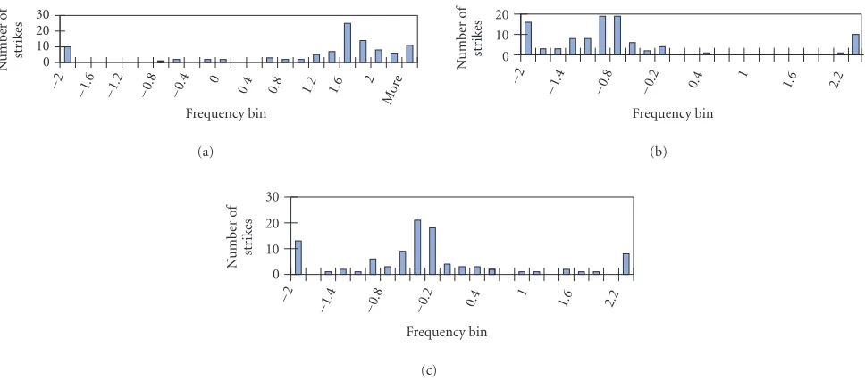
The histograms of the bootstrap estimates of the three parameters, using the stochastic-calculus-based method, are
shown in Figure 2. The approximate Cram´er-Rao lower
bound for the variances, the variances of the estimates of the coefficients of the polynomial phase using stochastic-calculus-based method, and the approximated maximum likelihood method are shown inFigure 3.
The mean square error (MSE) between the estimated pa-rameters and the true papa-rameters is taken as a measure of performance. The MSE for the ith coefficient is defined as
MSEi= 1
M
M
m=1
ami −ai
2
, (89)
whereMis the total number of the bootstrap simulations and is equal to 100,ami is themth estimate of theith coefficient
which is the peak of the histogram of this coefficient. InTable 1, we present the log value of the approximated Cram´er-Rao lower bound (CRB) and the log of the MSE val-ues for the stochastic-calculus-based method with bootstrap-ping for SNR value of 20 dB, 10 dB, and 0 dB. Notice how close they are.
4.2. Effect of bootstrapping
0 10 20 30
Nu
m
b
er
o
f
st
ri
ke
s
−2 −1.6 −1.
2 −0.
8 −0.
4 0
0.4 0.8 1.2 1.6 2 Mo
re
Frequency bin (a)
0 10 20
Nu
m
b
er
o
f
st
ri
ke
s
−2 −1.
4 −0.
8 −0.
2
0.4 1 1.6 2.2
Frequency bin (b)
0 10 20 30
Nu
m
b
er
o
f
st
ri
ke
s
−2 −1.
4 −0.
8 −0.
2
0.4 1 1.6 2.2
Frequency bin (c)
Figure 2: (a) Histogram of estimated f1 using stochastic-calculus-based method, the maximum value of the histogram at 1.6, SNR =
0 dB. (b) Histogram of estimated f2using stochastic-calculus-based method, the maximum value of the histogram at−1, SNR=0 dB. (c)
Histogram of estimatedf3using stochastic-calculus-based method, the maximum value of the histogram at−0.4, SNR=0 dB.
with bootstrap and the proposed stochastic-calculus-based method with bootstrap, are compared. Notice that using the bootstrapping, as expected, lowers the MSE of the esti-mates.
Notice that the accuracy of the proposed bootstrap-ping and stochastic-calculus-based method is much higher than the approximate maximum likelihood method. The measure of accuracy is the mean square error of the esti-mate.
4.3. Could we use bootstrapping to improve the performance?
Bootstrap is a method that handles small samples and yields good estimates for the bias and the confidence intervals for the plug-in estimates (see Efron and Tibshirani [21], Za-man [22], Politis [23], Zoubir and Boashash [24]). It is not meant to be a method to improve the accuracy of the esti-mates. Using the peak of the histogram, generated from the bootstrapping method for each estimated parameter, as the desired estimate of the unknown parameter, however, one is able to get good estimates at lower SNR. This was ob-served in this report and in some other applications (see Souza and Neto [25], Abutaleb [26]). This could be explained from the fact that the bootstrapping samples are almost the same as Monte Carlo simulations. Thus, instead of having just one data set for the estimation, one has as many sam-ples as needed. More important, bootstrapping provides a reasonably good approximation to the density of the param-eter estimator. This is apparent from the histogram of each parameter ofFigure 2. If the distribution of each parameter was Gaussian, then one should take the mean of the his-togram to be the best estimate of the unknown
parame-ter. But as we notice from (71) and Section 3.3, the dis-tribution of the estimates, f, is not Gaussian. This is true since the estimate ofγcomes into this equation. Thus, one might expect the density of f to be skewed. This is ex-actly what we observe in the histograms ofFigure 2. Choos-ing the peak of the histogram, as an estimate for the un-known parameter, is the reason for the improved accuracy and the lowering of the MSE. More discussion on this sub-ject could be found in [22, Chapters 12 and 14]. Again this is not a mathematical explanation for this observa-tion. More theoretical analysis is needed to explain why the peak yielded better estimates. This is currently under investigation.
Table 3lists, for SNR= 0 dB and for a typical group of bootstrapping estimates, the true value of the unknown pa-rameter, the plug-in estimate, the bias, the average, the vari-ance, and the peak of the histogram for each parameter. An estimate of the bias is obtained from the bootstrap estimates. It is defined as follows (Efron and Tibshirani [21, Chapter 10]): bias is equal to the average of the bootstrap estimates of the unknown parameter—the plug-in estimate of the un-known parameter.
5. SUMMARY
−3.5
−3
−2.5
−2
−1.5
−1
−0.5
0
Lo
g
scale
20 10 0
SNR (dB) CRBf1
MSE stochastic-calculusf1
MSE approximate MLf1
(a)
−2.5
−2
−1.5
−1
−0.5
0
Lo
g
scale
20 10 0
SNR (dB) CRBf2
MSE stochastic-calculusf2
MSE approximate MLf2
(b)
−2.5
−2
−1.5
−1
−0.5
0
Lo
g
scale
20 10 0
SNR (dB) CRBf3
MSE stochastic-calculusf3
MSE approximate MLf3
(c)
Figure3: (a) Approximate CRB and MSE of the stochastic-calculus-based estimate off1. (b) Approximate CRB and MSE of the
stochastic-calculus-based estimate of f2. (c) Approximate CRB and MSE of the stochastic-calculus-based estimate off3.
Table1: Log of the approximate CRB and the MSE of the stochastic-calculus-based method with bootstrapping. SNR values vary from 20 dB down to 0 dB.
Coefficient (SNRCRB= 20 dB)
CRB (SNR=
10 dB)
CRB (SNR=
0 dB)
MSE of stochastic calculus with bootstrapping
(SNR=20 dB)
MSE of stochastic calculus with bootstrapping
(SNR=10 dB)
MSE of stochastic calculus with bootstrapping
(SNR=0 dB)
f1 −3.2 −2.4 −1.9 −2.9 −2.4 −1.6
f2 −1.9 −1.3 −0.8 −1.9 −1.2 −0.8
f3 −2.3 −1.7 −1.4 −1.9 −1.5 −1.3
equation in some of the unknown parameters of the phase; an advantage of using Ito calculus. A pseudo-likelihood func-tion was obtained using the Girsanov theory. It was shown that the pseudo-likelihood function is quadratic in some of the unknown coefficients of the phase. This made it possi-ble to find an exact expression for the estimates of the pa-rameters of the polynomial phase; another advantage of the Ito calculus. The statistical properties of the estimates were also derived in a straightforward manner and an approxi-mate expression for the Cram´er-Rao lower bound was