An Application of MAP-MRF to Change Detection
in Image Sequence Based on Mean Field Theory
Qiang Liu
Laboratory for Computational Neuroscience, Departments of Neurological Surgery and Electrical Engineering, University of Pittsburgh, Pittsburgh, PA 15213, USA
Email:[email protected]
Robert J. Sclabassi
Laboratory for Computational Neuroscience, Departments of Neurological Surgery and Electrical Engineering, University of Pittsburgh, Pittsburgh, PA 15213, USA
Email:[email protected]
Ching-Chung Li
Laboratory for Computational Neuroscience, Departments of Neurological Surgery and Electrical Engineering, University of Pittsburgh, Pittsburgh, PA 15213, USA
Email:[email protected]
Mingui Sun
Laboratory for Computational Neuroscience, Departments of Neurological Surgery and Electrical Engineering, University of Pittsburgh, Pittsburgh, PA 15213, USA
Email:[email protected]
Received 24 December 2003; Revised 22 October 2004
Change detection is one of the most important problems in video segmentation. In conventional methods, predetermined thresh-olds are utilized to test the variation between frames. Although certain reasonings about the threshthresh-olds are provided, appropriate determination of these parameters is still problematic. We present a new approach to change detection from an optimization point of view. We model the video frames and the change detection map (CDM) as Markov random fields (MRFs), and formulate change detection into a problem of seeking the optimal configuration of the CDM. Under the MRF assumption, the optimal solu-tion, in the sense of maximum a posteriori (MAP), is obtained by minimizing the energy function associated with the MRF which is designed by utilizing the prior knowledge of noise and contextual constraints on the video frames. An algorithm that computes the potentials and optimizes the solution is constructed by applying the mean field theory (MFT). The experimental results show that the new method detects changes accurately and is robust to noise.
Keywords and phrases:change detection, image processing, Markov random field, mean field theory, video segmentation.
1. INTRODUCTION
Content-based video processing has been widely studied and is supported by a number of standards, such as MPEG-4 for video object-based compression and MPEG-7 for video con-tent description [1,2]. These standards involve functional-ities that rely on segmenting video sequences into semantic regions or video objects. Change detection, which generates an initial segmentation mask, usually constitutes the first step of video segmentation [3,4].
Much research effort has been devoted to change detec-tion in recent years [5,6, 7, 8]. Most existing approaches focus on thresholding which contains two essential steps of defining a metric function of intensity variation and
choos-ing a proper threshold to be applied to the metric function. The key issue of these methods is to determine the thresh-old. However, it is often problematic choosing the threshold, since a large threshold removes noise as well as the signal (change caused by motion), while a small threshold makes the detection sensitive to noise. One way to determine the threshold is to introduce contextual constraints. Aach pro-posed a multiple-threshold approach from a framework of maximum a posteriori (MAP) estimation [9]. Unfortunately, this method in general does not provide a MAP solution, be-cause the thresholds are chosen in a deterministic fashion.
problem in a global perspective. If we take the change de-tection map (CDM) as a 2D binary random field, then la-beling each pixel as “changed” or “unchanged” becomes a problem of finding an appropriate configuration of this ran-dom field. This concept may be implemented by employing Markov random fields (MRF) theory, which is a well-known model in describing image characteristics [10]. In general, this theory says that the value of a random variable at one site in a MRF is only affected by the values of variables at its neighboring sites (determined by a neighborhood sys-tem that is defined). If one can describe the interactions be-tween the neighboring sites, then it is possible to obtain a global description of the whole field. Moreover, if an a pri-ori of image characteristics is applied in describing the in-teraction between neighboring sites (pixels), then one may obtain an optimal solution associated with the MRF in MAP sense [11]. For the change detection problem, the interac-tion between neighboring sites can be translated into con-textual constraints between neighboring pixels. A simple ex-ample would be the constraint of smoothness, which means that the neighboring pixels of a changed/unchanged pixel are likely to be changed/unchanged too. These contextual con-straints come from prior knowledge of our assumption on the image sequence being analyzed. Based upon this knowl-edge, the CDM from a pair of frames can be appropriately modeled as MRFs, by choosing the neighborhood system and formulating the impact between the neighboring sites. The rest of the task is then to search for a configuration of the CDM that satisfies the MAP criterion. In the literature, there are several methods to perform this search using, for exam-ple, simulated annealing and iterative conditional mode al-gorithms [12,13]. The former aims at providing the global extremum, but requires extensive computation; the latter re-duces the computational cost, but may converge to a local extremum. We adopt the mean field theory (MFT) approach as studied recently in [14,15], which trades offbetween these two approaches.
This paper is organized as follows: Section 2 gives a brief review of the related theories; Section 3describes the proposed methods and algorithms of change detection; Section 4presents the experimental results based on the pro-posed method; andSection 5provides a conclusion.
2. BACKGROUND THEORIES
Fundamentals of the MRF and the MFT are briefly intro-duced in this section.
2.1. Markov random field theory in change detection
Let ¯F= {F1,2,. . .,Fi,j,. . .,Fm,n}be a 2D random array, where
Fi,j, 1 ≤ i ≤ m, 1 ≤ j ≤ n, is a random variable at site (i,j). LetS = {(i,j)|1 ≤ i ≤ m, 1 ≤ j ≤ n}be the set of all sites. Frame ¯f = {fi,j, (i,j)∈S}is a realization of ¯F. Let
p( ¯f) denote the joint probability density function (pdf) of ¯
F = f¯, where p( ¯f)= p{F¯ = f¯} = p{F
i,j = fi,j, (i,j)∈S}. Then, with the same notation, ¯F is a MRF if (1) p( ¯f) > 0, for all ¯f ∈ F¯, and (2) p(fi,j|fS) = p(fi,j|fN
i,j), where
(i, j)
(a) (b) (c)
Figure 1: (a) A first-order neighborhood system, (b) single-site clique, and (c) double-site cliques.
S = S−(i,j), with symbol “−” denoting exclusion, and
Ni,j= {(i,j)|(i−i)2+ (j−j)2≤k, (i,j)∈S}, withk being a positive integer.Ni,j defines the set of thekth order neighboring sites of (i,j). With the definition ofNi,j, a clique, denoted byc, is defined as a set containing single or multiple sites that are connected withinNi,j, (i,j)∈S.Figure 1 illus-trates an example of cliques of a first-order neighborhood, wherecmay be a collection of single sites or double sites. It was introduced in [16] that the joint pdfp( ¯f) may be ap-proximated by the Gibbs distribution:
p( ¯f)=e−(1/T)U( ¯f)
¯
fe−(1/T)U( ¯f)
, (1)
whereTis a constant andUis an energy function of the MRF given by
U( ¯f)= c
Vc( ¯f) (2)
withVc’s being clique potentials or clique functions. TheVc functions represent contributions to the total energy from single-site cliques, double-site cliques, and so forth. Note that (1) and (2) reflect the fact that the global identityp( ¯f) is de-termined by the local activities, namely, the clique potentials. Considering the first-order neighborhood, we may rewrite (2) into the following form [11]:
U( ¯f)=
(i,j)
V(i,j)
fi,j
+V{(i,j),(i+1,j)}fi,j,fi+1,j
+V{(i,j),(i,j+1)}fi,j,fi,j+1
,
(3)
where the first, second, and third term are single-site, horizontal double-site, and vertical double-site clique potentials, respectively. Notice that for a double-site clique {(i,j), (i,j)}, the associated clique potentials
V{(i,j),(i,j)}(fi,j,fi,j) and V{(i,j),(i,j)}(fi,j,fi,j) are equal. Therefore, (3) may be rearranged into
U( ¯f)=
(i,j)
Vc1
fi,j
+1 2
(i,j)∈Ni,j
Vc2
fi,j,fi,j
=
(i,j)
Ui,j
fi,j
,
wherec1andc2are single-site and double-site cliques in the
defined neighborhood, and Ui,j(fi,j) is the energy function associated with site (i,j). As pointed out in [11], ifp( ¯f) is a posterior distribution, minimizing the energy functionU( ¯f) yields a MAP estimate of the joint pdfp( ¯f).
2.2. Mean field theory
To make the MRF theory more practical, we need to intro-duce the MFT. From the description of the MRF, we know that the value assigned to a random variable in the MRF is af-fected by the values at its neighboring sites, which are further dependent on their neighbors. One way to calculate the inter-action between one site and its neighbors is to apply the MFT [14,17], which assumes that the impacts from the neighbors can be approximated by an average field. We denote the mean field for site (i,j) by fimf,j . As a result, if the first-order neigh-borhood is considered, one may write the energy function related to site (i,j) in the following form [14]:
Uimf,j
fi,j
=Vc1
fi,j
+
(i,j)∈Ni,j
Vc2
fi,j,fimf,j
, (5)
whereVc1(·) andVc2(·,·) are potential functions of single-site and double-single-site cliques, respectively; andfimf,jis the mean field for fi,j. Then, the marginal distribution of the MRF at site (i,j) may be approximated by [14]
pfi,j
= 1
fi,je
−(1/T)Umf
i,j(fi,j)e
−(1/T)Umf
i,j(fi,j). (6)
As seen from (4) and (5), the energy function is decom-posed into local computations, where each site is treated in-dependently. Therefore, the joint pdf p( ¯f) can be approxi-mated by
p( ¯f)≈ i,j
pfi,j
. (7)
Then, maximizingp( ¯f) is equivalent to maximizing each
p(fi,j), or, to minimizing the correspondingUimf,j(fi,j). In order to evaluateUimf,j(fi,j), the mean field values fimf,j at the neighboring sites (i,j) withinNi,jmust be computed. The general way to calculate a mean field value is by the fol-lowing form:
fmf
i,j =
fi,j
fi,j·p
fi,j
. (8)
Note that (8) requires the evaluation of p(fi,j), henceforth,
Umf
i,j(fi,j). Therefore, the computation of the mean field value is usually carried out by iteration that stops when the change of the results from two consecutive iterations is sufficiently small.
3. MRF CHANGE DETECTION METHOD
3.1. MAP-MRF in change detection
We denote the CDM by ¯H = {H1,2,. . .,Hi,j,. . .,Hm,n}, and
¯
h = {h1,2,. . .,hi,j,. . .,hm,n} a configuration of ¯H, where
hi,j∈ {−1, 1}, (i,j)∈Swith “−1” denoting unchanged and “1” denoting changed. Then, given two frames ¯f(0)and ¯f(1),
our goal is to find the optimal ¯h∗in the MAP sense, such that ¯
h∗=argmax¯hph¯|f¯(0), ¯f(1)
=argmax¯h p
¯
f(1)|f¯(0), ¯h·ph¯|f¯(0)
pf¯(1)|f¯(0)
=argmax¯hpf¯(1)|f¯(0), ¯h·ph¯|f¯(0).
(9)
Applying MRF assumption on both ¯Fand ¯H, maximiz-ingp(¯h|f¯(0), ¯f(1)) with respect to ¯his equivalent to
minimiz-ing its energy functionU(¯h|f¯(0), ¯f(1)). This, as suggested by
(9), can be accomplished by minimizing the energy func-tions U( ¯f(1)|h¯, ¯f(0)) and U(¯h|f¯(0)), which are associated
with p( ¯f(1)|f¯(0)) and p(¯h|f¯(0)), respectively.U( ¯f(1)|h¯, ¯f(0))
addresses the potential of the likelihood between ¯f(1) and
¯
f(0) with the knowledge of ¯h, that is, whether the sites are
changed. And, U(¯h|f¯(0)) is always considered to represent
the spatial domain constraints, for example, the smoothness or similarity between neighboring sites. Therefore, a general form of the prior model of these energy functions is
Uh¯|f¯(0), ¯
f(1)=γfU ¯
f(1)|h¯, ¯f(0)+
γhU ¯
h|f¯(0), (10)
whereγf andγhare regularization parameters. The larger the regularization parameter values, the more the corresponding constraint is emphasized.
Equivalently, we can write (10) by
Uh¯|f¯(0), ¯f(1)=γf
Uf¯(1)|h¯, ¯f(0)+γUh¯|f¯(0), (11)
where γ = γh/γf. It is noticed that to minimize
U(¯h|f¯(0), ¯f(1)) with respect to ¯his equivalent to minimizing
U( ¯f(1)|h¯, ¯f(0)) +γU(¯h|f¯(0)). Therefore, we define the energy
function in the following form:
Uh¯|f¯(0), ¯f(1)=Uf¯(1)|h¯, ¯f(0)+γUh¯|f¯(0). (12)
In change detection, we interpretU( ¯f(1)|h¯, ¯f(0)) as the
sum of single-site clique potentials, which is
Uf¯(1)|h¯, ¯f(0)=
c1
Vc1 ¯
f(1)|h¯, ¯f(0)
=
i,j
Vc1
fi,(1)j |hi,j,fi(0),j
, (13)
whereVc1is selected to be
Vc1
fi,(1)j |hi,j,fi(0),j
= −lnpdi,j|hi,j
(14)
which is the negative of the natural logarithm of the pdf of the absolute frame differencedi,j= |fi(1),j −fi(0),j |at site (i,j)∈
S, given the knowledge ofhi,j. Therefore, ifdi,jis consistent with the prior belief, the conditional probability will be high. As a result, its logarithm value will be low, and vice versa, as required by the design rules. Choosing the natural loga-rithm is instinctive. First, more penalty would be assigned to smaller probability, for example, when probability is close to zero, the value of energy function would be extremely large. Second, considering p( ¯f(1)|f¯(0), ¯h = −1), which is
equiva-lent to the pdf of frame difference caused by noise, we may assume p( ¯f(1)|f¯(0), ¯h = −1) =
i,jp(di,j | hi,j = −1), or
i,jZi,j·e−(1/T)Vc1(f (1)
i,j|hi,j=−1,fi(0),j ) =
i,jp(di,j | hi,j = −1), whereZi,j are normalization constants. Furthermore, if the noise distributionp(di,j |hi,j = −1) also has an exponential form, such as Gaussian and Laplacian, we may reasonably take the natural log on both sides of the above equation to get the potential function. For the case ofhi,j = 1, that is, with the presence of change, the independence assumption may not hold in general. However, this assumption can be accepted as a reasonable simplification to trade off computa-tional complexity [18]. Therefore, the above reasoning may also apply to the casehi,j=1. The collection of prior knowl-edge will be described inSection 3.2.
The other energy function U(¯h|f¯(0)) in (10) addresses
the contextual constraints on the neighboring sites. This can be explained as follows: with the knowledge of ¯f(0), we want
to obtain ¯hthat complies with the properties of ¯f(0), for
ex-ample, the continuity of ¯hif we assume that ¯f(0)is smooth.
Based upon this reasoning, we define
Uh¯|f¯(0)=
i,j
c2⊂Ni,j
Vc2 ¯
h|f¯(0)
=
i,j
1 2
(i,j)∈Ni,j
Vc2
hi,j,hi,j
,
(15)
wherec2is a double-site clique in a first-order neighborhood
Ni,jat site (i,j)∈S. The scaling factor 1/2 has been explained in (3) and (4). The clique potentialVc2(·,·) is defined as
Vc2
hi,j,hi,j= −ln1−0.5hi,j−λ·hi,j, (16) whereλ∈(0, 1) is a constant representing the impact of site (i,j) on site (i,j). The reasons behind this design are (1)
we want the state of site (i,j) to agree with its neighboring sites; (2) the logarithm form is consistent with that in (14). The term 1−0.5|hi,j−λ·hi,j|acts as a probability of the random variable at site (i,j) when its value agrees with those at its neighboring sites. Therefore, this definition also follows the design rules stated previously.
To minimizeU(¯h|f¯(0), ¯f(1)), we must evaluate the clique
potential functions. A question now is how to calculate
Vc2(hi,j,hi,j). As mentioned previously, we may apply MFT to simplify this calculation. If the first-order neighborhood system is assumed, we have the following approximation:
Uh¯|f¯(0)≈
i,j
(i,j)∈Ni,j
Vc2
hi,j,hmfi,j
, (17)
where
Vc2
hi,j,hmfi,j
= −ln1−0.5hi,j−λ·hmfi,j. (18) Combining (10)–(18), we have
Uh¯|f¯(0), ¯f(1)≈
i,j
Uimf,j
hi,j|fi(0),j ,fi(1),j
, (19)
where
Umf
i,j
hi,j|fi(0),j ,f
(1)
i,j
= −lnpdi,j|hi,j
− γ
(i,j)∈Ni,j
ln1−0.5hi,j−λ·hmfi,j .
(20)
Essentially, to minimizeU(¯h|f¯(0), ¯f(1)), we only need to
evaluateUimf,j(·) at each site (i,j), and choosehi,jbetween−1 and 1 to render a smaller value ofUmf
i,j(·).
3.2. The MRF change detection algorithm
Equation (20) requires evaluation of p(di,j|hi,j), (i,j) ∈ S. Instead of collecting the pdf for each site, we utilize the same pdf, denoted byp(d|h), for all sites, wheredandhhave the same sample spaces asdi,jandhi,j, respectively. This choice is motivated from a practical point of view, since it would be extremely expensive to allocate memory forp(di,j|hi,j) for each (i,j)∈S. Whenh(i,j)= −1, this approximation can be justified because the value differences of unchanged sites are driven by noise, which is usually considered to be in-dependently and identically distributed. For moving pixels, the above assumption is not true in general. However, if we assume that each pixel may experience the same or similar amounts of motion, the validity of using p(d|1) for all the sites is also justifiable.
To trainp(d| −1), we utilize the video segments contain-ing motionless scenes. This is relatively easy to accomplish in many applications, such as in surveillance and teleconfer-ence videos. In general, it is difficult to train p(d|1); how-ever, it is possible to train a prototype for specific applica-tions. Practically, we adopt the following strategy to calculate
across the entire range of its sample space, that is, p(d|1)= 1/(L+ 1), d ∈ [0,L] for a discrete case; then, starting with the initial value, we adaptp(d|1) during a detection process, using the following equation:
p(r)d|1=(1−·ρ)·p(r−1)d|1+·ρ·p(dr|)1, (21)
where p(r)(d|1) and p(r−1)(d|1) are the pdf p(d|1) adapted
from frame 1 to framesr andr−1, respectively,p(dr|)1is the
pdf of the changed pixels contained in framer,ρis the ratio of the number of changed pixels to the total number of pixels in that frame, and∈(0, 1) is a control parameter. The term
ρreflects the intuition that the more changed pixels there are, the morep(d|1) should be adapted. Parameteris designed to control the rate of adaptation.
An important question now is how the mean field value
hmf
i,j, (i,j)∈Sis evaluated. As mentioned before, the mean field value is usually computed iteratively until it converges. As described inSection 2.2, with the local energy function
Umf
i,j(hi,j|fi(0),j ,fi(1),j ),hmfi,j can be evaluated by
hmf
i,j =
hi,j
hi,j· e
−(1/T)Umf
i,j(hi,j|fi(0),j,f
(1)
i,j)
hi,je
−(1/T)Umf
i,j(hi,j|fi(0),j,fi(1),j).
(22)
Applying (20), we have
e−(1/T)Uimf,j(hi,j|fi(0),j,fi(1),j)
=
pd|h·
(i,j)∈Ni,j
1−0.5hi,j−λhmfi,j γ 1/T . (23)
Note that the computing time can be greatly reduced by using (23). The iteration continues until the following condition is satisfied:
1
m·n
i,j hmf
i,j(k+ 1)−himf,j(k)< θ, (24)
wherekis the index of iteration,m·nis the total number of pixels, andθ∈(0, 1) is a chosen threshold.
With these assumptions and simplifications, we present Algorithm 1to implement the proposed model.
4. IMPLEMENTATION AND EXPERIMENTS
In this section, the experimental results based on the pro-posed method are reported. We present the results of two types of data: a synthetic image sequence generated by us-ing Matlab (version R12, MathWorks Inc., Mass) and a se-lected set of the reference MPEG test sequences available in the public domain (e.g.,http://sampl.eng.ohio-state.edu/
∼sampl/database.htm,http://www.neuronet.pitt.edu/∼qliu/ Links.htm). All the sequences are in the QCIF format (144× 176 in size). Only the Y component is utilized to calculate frame differences.
Step 1. Loadp(d| −1) and initialize p(d|1)=1/256, ford=0, 1,. . ., 255. Assign values toγ,λ,, andθ. Step 2. Take two frames ¯f(0)and ¯f(1), and
calculate ¯d= |f¯(0)−f¯(1)|; initialize
mean field values ¯hmf, where for each
pixel (i,j),hmf
i,j =0.
Step 3. For each pixel (i,j), evaluate (20) with hi,j= −1 and 1, and calculate the new mean field value by (22) and (23). Step 4. Evaluate the difference between the new
mean field value and the previous one as defined in (24); if the difference is less thanθ, then go to next step, otherwise go to step 3.
Step 5. For each pixel, if the local energy Umf
i,j(hi,j= −1|fi,(0)j ,f
(1)
i,j )> Uimf,j(hi,j= 1|fi(0),j ,fi,(1)j ), then label pixel (i,j)
unchanged, otherwise changed. Step 6. Updatep(d|1) by (21); finish if all the
frames are done, otherwise go to step 2.
Algorithm1: MRF-MFT change detection algorithm.
Table1: Typical control parameters.
Parameter T γ λ θ
Value 2 1 0.99 0.5 0.05
As described previously, five controlling parametersT,γ,
λ,, andθare required.Table 1lists typical values of these parameters, which were chosen experimentally and utilized for all the test sequences. In the following, we describe these parameters individually.
(i) Tis called “temperature” in MRF-based methods, for example, simulated annealing algorithm [12]. This pa-rameter determines the spread of the Gibbs distribu-tion. The larger theT, the more it spreads. In sim-ulated annealing,T is gradually decreased. However, as suggested by [19], a fixed T is able to render a satisfactory result while reducing the computational cost. Therefore, a constantTwas utilized throughout our experiments.
(ii) γ is a regularization parameter to balance the con-straints introduced by different clique potentials. In our application, a large γ value emphasizes the smoothness constraint.
(iii) λ models the impact between neighboring sites. In (16),hi,j−λhi,jis utilized to represent the difference between neighboring sites (i,j) and (i,j). The value ofλcontrols the degree of impact from (i,j). (iv) is utilized to control the adaptation of the pdf ofdin
the presence of change. The larger the value of, the more the pdf adapts to each CDM, and the faster the adaption to test data. However, considering the risk of false detection, we assigna moderate value.
(a) (b) (c) (d)
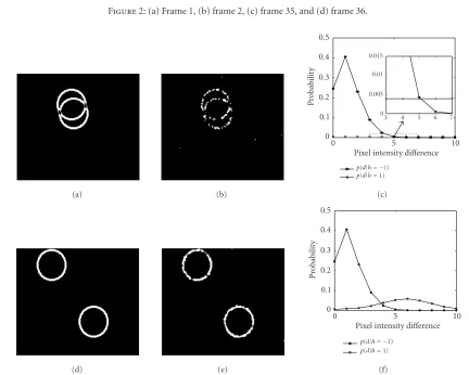
Figure2: (a) Frame 1, (b) frame 2, (c) frame 35, and (d) frame 36.
(a) (b)
10 5
0
Pixel intensity difference 0
0.1 0.2 0.3 0.4 0.5
P
robabilit
y
7 6 5 4 3 0 0.005 0.01 0.015
p(d|h= −1)
p(d|h=1)
(c)
(d) (e)
10 5
0
Pixel intensity difference 0
0.1 0.2 0.3 0.4 0.5
P
robabilit
y
p(d|h= −1)
p(d|h=1)
(f)
Figure3: The upper plots represent the change detection results from frames 1 and 2: (a) the known CDM, (b) the detected CDM, and (c)
p(d|h= −1) and initialp(d|h=1). The subplot embedded in (c) shows a close-look of the marked region (by the dashed line). The lower
plots represent the change detection results from frames 35 and 36: (d) the known CDM, (e) the detected CDM, and (f)p(d|h= −1) and
p(d|h=1) (adapted from frames 1∼35).
4.1. Synthetic data
To evaluate the new change detection method quantitatively, we generated a synthetic image sequence by using Matlab in the following way: a circle (with a radius of 20, line width of 3, both in pixels, and gray-level intensity of 5) is plotted in a frame; then, white Gaussian noise with mean 127 and stan-dard deviation 1.6 is added to each frame. It should be noted that the signal-to-noise (SNR) ratio of the synthetic data, de-fined as 20 log(circle intensity/noise standard deviation), is less than 10 dB, which is much lower than the SNR in most natural videos. The coordinates of the origins were ran-domly generated. Two pairs of sample frames are shown in
Figure 2. We denote the ground truth CDM by ¯h(r), the
de-tected CDM by ¯h(t), and the set of sites with false labels by
Se = {(i,j)|h(i,rj) = h
(t)
i,j, (i,j) ∈ S}. The error rate is then defined as
Er= Se
S , (25)
where Se and S denote the number of sites inSeandS, respectively.
(a) (b) (c) (d)
Figure4: (a), (b) The CDMs detected by “quadratic picture function” (QPF) method: (a) CDM from frames 1 and 2; (b) CDM from frames 35 and 36. (c), (d) The CDMs detected by the method of De Geyter and Philips (M3 method): (c) CDM from frames 1 and 2; (d) CDM from frames 35 and 36.
50 40
30 20
10 0
Frame number 0
0.02 0.04 0.06
Er
ro
r
rat
e
MRF QPF M3
Figure5: The error rates of our method MRF, the quadratic picture function method (QPF), and the method of De Geyter and Philips (M3).
detected CDM, and p(d|h = −1) and the initial p(d|h = 1), respectively. Compared with the ground truth CDM, the detected CDM has visible false detections. However, with the adaption of p(d|h=1), the false detections are reduced. As seen in the lower plots, where the results were obtained from frame 35 and 36, the detected CDMFigure 3econtains much less false detections. InFigure 3fit can be seen thatp(d|h= −1) was kept intact because of the assumption of stationary noise, butp(d|h=1) was adapted to a bell-shaped function according to (21).
To demonstrate the robustness of the MRF approach, we compare it with two existing methods, quadratic picture function (QPF) method developed by Hsu et al. [6], and a novel method (“Method 3,” abbreviated as M3 in the fol-lowing) recently presented by Geyter and Philips [20]. In the former method, the threshold value of 5.76 was selected,
which corresponds to a significant level of 0.005. In the lat-ter method, the paramelat-ters α,β, and z (see [20]) were set to 0.5, 0.9, and 3, respectively. The parameterkin M3 was tested from 2 to 5 andk =4 was selected, which produced the best overall performance for the test sequences. These pa-rameter values were utilized for all the test sequences (syn-thetic and natural). The results of QPF and M3 methods are illustrated in Figures4a-4band4c-4d, respectively. Com-pared with the CDMs shown in Figure 3, these two meth-ods appear to be more sensitive to the simulated noise. The error rates of the three methods are illustrated inFigure 5, which shows that the MRF method performed better than the two existing methods in terms of less false detection. It is seen that the error rate of the MRF method decreases as frames 1 through 30 are being processed, then becomes sta-ble after that. The reason is thatp(d|h=1) adapts gradually to the test data at the initial frames, and then becomes sta-tionary. The adaptation speed is quite satisfactory for most common applications, as indicated by our results using other videos.
4.2. Real-world data
In this section, experimental results on selected MPEG test sequences are presented. Change detection was carried on these sequences at a rate of 10 frame pairs per second. First, we report the experiment onMother & Daughtersequence by the proposed method.Figure 6shows frames 58 through 91 which contain both large motions (e.g., hand movement in frame 58 and 61) and small motions (e.g., chest and shoul-der movements). The detected CDMs are shown inFigure 7. It can be seen that the stationary background and the mov-ing objects are well distmov-inguished. The background area is quite clean, indicating that the MRF method is robust to the salt and pepper noise contained in this sequence. Figure 8 depicts the pdf ’s calculated from this sequence. While pdf
(a) (b) (c) (d)
(e) (f) (g) (h)
(i) (j) (k) (l)
Figure6: Frames ofMother & Daughtersequence. (a)–(l) Frames 58, 61, 64, 67, 70, 73, 76, 79, 82, 85, 88, and 91.
(a) (b) (c) (d)
(e) (f) (g) (h)
(i) (j) (k) (l)
10 5
0 0 0.1 0.2 0.3 0.4 0.5
p(d|h= −1)
p(d|h=1) at frame no. 60
p(d|h=1) at frame no. 1
p(d|h=1) at frame no. 300
p(d|h=1) at frame no. 600
p(d|h=1) at frame no. 900
P
robabilit
y
Pixel intensity difference
(a)
4 3
2 1
0 0 0.1 0.2 0.3 0.4 0.5
p(d|h= −1)
p(d|h=1) at frame no. 60
p(d|h=1) at frame no. 1
p(d|h=1) at frame no. 300
p(d|h=1) at frame no. 600
p(d|h=1) at frame no. 900
P
robabilit
y
Pixel intensity difference
(b)
Figure8: The pdf ’s obtained from Mother & Daughter sequence. (a) p(d|h= −1) and p(d|h= 1) at frames 1, 60, 300, 600, and 900. (b) A close look at the pdf ’s in the marked range (by the dashed line) in (a).
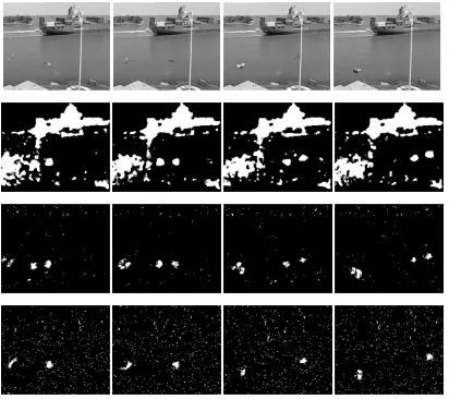
Figure10: Experimental results on test sequenceContainer. From top to bottom: frames 252, 255, 258, and 261; CDMs detected by the MRF method, by the QPF method, and by the M3 method.
In the following, the comparisons with QPF and M3 methods are reported. Several representative change detec-tion results on Miss America,Container,Table Tennis, and News are shown in Figures9–12. In the selected frames of Miss America (Figure 9), the subject’s head and body were moving to her left. It can be observed that the CDMs de-tected by the MRF approach reflected this motion, where changes in the face region were very well detected. The results from QPF captured most of the changes; however, the dis-turbance from noise appeared in the background area. The CDMs detected by M3 had certain errors and also suffered from noise.
The results on the container sequence, a typical outdoor video, are presented inFigure 10. In the sample frames, the container was moving slowly to the right and two birds flew by quickly from the left to the right. It can be seen that all the three methods captured the changes caused by the flying birds. However, the motions of the container and rippling water were only well identified by the MRF method, which shows that the proposed method is more efficient in detect-ing small changes than the other two methods.
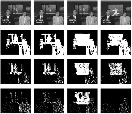
Figure 11demonstrates the results on the table tennis se-quence, which contains very fast motion. Again, the MRF method detected moving regions more completely than the other two methods. The scenes selected in news sequence contain both small motion (e.g., face of the male journal-ist) and large motion (e.g., the spinning stage and dancers). It can be seen inFigure 12that, although all three methods were robust against background noise, the MRF approach was superior to the other two methods in detecting more completely changing regions, including both the journalists and the moving stage and dancers.
Figure11: Experimental results of the test sequenceTable Tennis. From top to bottom: frames 132, 135, 138, and 141; CDMs detected by the MRF method, by the QPF method, and by the M3 method.
pixels contained in a video frame, and therefore is largely fixed for all the testing sequences. The computing time of the MRF depends not only on the spatial resolution, but also the number of iterations taken to compute the mean field values. In practice, if the time of computation is critical, a maximum number of iterations can be specified. For exam-ple, our system required an average of 9.4 milliseconds per iteration, so a maximum number of iterations of 10 was uti-lized in detecting changes in image sequence at 10 frames per second.
5. CONCLUSION
In this paper, we have presented a new approach to the change detection problem in image sequences. This approach employs two well-established theories: MRF and MFT. Based upon the MRF theory, change detection is modeled as an optimization problem, namely, the CDM is calculated in the sense of MAP. Our approach differs from the previous
statistical methods which rely on thresholding. In order to carry out an efficient computation, we utilized MFT, which simplifies the procedure of searching for the optimal detec-tion of CDM. Experimental results are reported based on this optimization approach. Both the synthetic and real-world data indicate that this approach accurately detects changes between frame pairs. One remaining problem, however, is to determine the values of control parameters in the associated functions. Currently, the parameters are chosen in an exper-imental manner. In the future, a meaningful cost function of these parameters may be designed to provide the values in a certain optimal sense.
ACKNOWLEDGMENT
Figure12: Experimental results onNews. From top to bottom: frames 84, 87, 90, and 93; CDMs detected by the MRF method, by the QPF method, and by the M3 method.
Table2: Computational cost of MRF, QPF, and M3 methods.
Test sequence MRF (average loops/time) QPF (time) M3 (time)
Miss America 4.31 loops/40.51 ms 147.2 ms 5.56 ms
Container 6.49 loops/61.0 ms 147.2 ms 5.56 ms
Table Tennis 5.37 loops/50.48 ms 147.2 ms 5.56 ms
News 3.93 loops/36.94 ms 147.2 ms 5.56 ms
REFERENCES
[1] MPEG-4 Video Verification Model Version 15.0, ISO/IEC JTC1/SC29/WG11 N3093,1999.
[2] T. Sikora, “The MPEG-7 visual standard for content descrip-tion an overview,”IEEE Trans. Circuits Syst. Video Technol., vol. 11, no. 6, pp. 696–702, 2001.
[3] T. Meier and K. N. Ngan, “Segmentation and tracking of
mov-ing objects for content-based video codmov-ing,”IEEE Trans.
Cir-cuits Syst. Video Technol., vol. 9, no. 8, pp. 1190–1203, 1999. [4] M. Kim, J. G. Choi, D. Kim, et al., “A VOP generation tool:
au-tomatic segmentation of moving objects in image sequences
based on spatio-temporal information,”IEEE Trans. Circuits
Syst. Video Technol., vol. 9, no. 8, pp. 1216–1226, 1999. [5] K. Skifstad and R. Jain, “Illumination independent change
detection for real world image sequences,”Computer Vision,
Graphics and Image Processing, vol. 46, no. 3, pp. 387–399, 1989.
[6] Y. Z. Hsu, H. H. Nagel, and G. Rekers, “New likelihood test
methods for change detection in image sequences,”Computer
[7] T. Aach, A. Kaup, and R. Mester, “Statistical model-based change detection in moving video,”Signal Processing, vol. 31, no. 2, pp. 165–180, 1993.
[8] E. Durucan and T. Ebrahimi, “Change detection and
back-ground extraction by linear algebra,” Proc. IEEE, vol. 89,
no. 10, pp. 1368–1381, 2001.
[9] T. Aach and A. Kaup, “Bayesian algorithms for adaptive change detection in image sequences using Markov random fields,”Signal Processing: Image Communication, vol. 7, no. 2, pp. 147–160, 1995.
[10] R. Chellappa and A. Jain,Markov Random Fields Theory and
Applications, Academic Press, Boston, Mass, USA, 1993. [11] S. Geman and D. Geman, “Stochastic relaxation, Gibbs
distri-butions, and the Bayesian restoration of images,”IEEE Trans.
Pattern Anal. Machine Intell., vol. 6, no. 6, pp. 721–741, 1984. [12] S. Kirkpatrick, C. D. Gellatt, and M. P. Vecchi, “Optimization by simulated annealing,”Science, vol. 220, no. 4598, pp. 671– 680, 1983.
[13] J. E. Besag, “On the statistical analysis of dirty pictures (with discussion),”Journal of the Royal Statistical Society. Series B, vol. 48, no. 3, pp. 259–302, 1986.
[14] J. Zhang, “The mean field theory in EM procedures for blind
Markov random field image restoration,”IEEE Trans. Image
Processing, vol. 2, no. 1, pp. 27–40, 1993.
[15] J. Wei and Z.-N. Li, “An efficient two-pass MAP-MRF
algo-rithm for motion estimation based on mean field theory,” IEEE Trans. Circuits and Systems for Video Technology, vol. 9, no. 6, pp. 960–972, 1999.
[16] M. Hassner and J. Sklansky, “The use of Markov random fields
as models of texture,”Computer Graphics and Image
Process-ing, vol. 12, no. 4, pp. 357–370, 1980.
[17] D. Chandler, Introduction to Modern Statistical Mechanics,
Oxford University Press, New York, NY, USA, 1987.
[18] L. Bruzzone and D. F. Prieto, “An adaptive semiparametric and context-based approach to unsupervised change
detec-tion in multitemporal remote-sensing images,” IEEE Trans.
Image Processing, vol. 11, no. 4, pp. 452–466, 2002.
[19] J. Zhang and G. G. Hanauer, “The application of mean field
theory to image motion estimation,”IEEE Trans. Image
Pro-cessing, vol. 4, no. 1, pp. 19–33, 1995.
[20] M. De Geyter and W. Philips, “A noise robust method for
change detection,” inProc. IEEE International Conference on
Image Processing (ICIP ’03), vol. 2, pp. 391–394, Barcelona, Spain, September 2003.
Qiang Liureceived his B.S. and M.S. degrees in telecommunications from Xidian Uni-versity, Xian, China, in 1996 and 1999, re-spectively. His research experience includes hardware and software designs in the State Key Lab on ISDN, Xidian University, Xian, China, and ZTE telecommunication cor-poration, Shanghai, China. He is currently a Ph.D. student at the University of Pitts-burgh, PittsPitts-burgh, USA. His recent research
has been on image representation, object-based video coding, biomedical signal processing, medical imaging, image understand-ing, and computer vision.
Robert J. Sclabassiis currently a Professor of neurological surgery, electrical engineer-ing, neuroscience, mechanical engineerengineer-ing, psychiatry, and biomedical engineering at the University of Pittsburgh. He completed his undergraduate education at Loyola Uni-versity of Los Angeles and earned his Mas-ters and Engineers degrees in electrical engi-neering at the University of Southern Cali-fornia. He was employed at TRW in a new
product development for approximately 8 years and is a profes-sional electrical engineer. He received a Ph.D. degree in electrical engineering from the University of Southern California in 1971 and then was a postdoctoral scholar studying basic and clinical neuro-physiology at the Brain Research Institution, University of Califor-nia, Los Angeles, before joining the faculty at that institution in the Departments of Neurology and Biomathemtics. In 1981, he earned an M.D. degree from the University of Pittsburgh. He has published over 330 articles and book chapters and 150 abstracts.
Ching-Chung Lireceived the B.S.E.E. de-gree from the National Taiwan University, Taipei, in 1954, and the M.S.E.E. and Ph.D. degrees from the Northwestern University, Evanston, Ill, in 1956 and 1961, respectively. He is presently a Professor of electrical engi-neering and computer science at the Univer-sity of Pittsburgh, Pittsburgh, Pa. He was a Visiting Professor of electrical engineering at the University of California, Berkeley, in
the spring of 1964, and a Visiting Principal Scientist at the Biody-namics Laboratory, Alza Corporation, Palo Alto, Calif, in the sum-mer of 1970. On his sabbatical leaves, he was with the Laboratory for Information and Decision Systems, Massachusetts Institute of Technology, in the fall of 1988, and with the Robotics Institute, Carnegie-Mellon University, in the spring of 1998. His research in-terests are in pattern recognition, image processing, biocybernet-ics, and applications of wavelet transforms. He is a Fellow of the IEEE.
Mingui Sunreceived a B.S. degree from the Shenyang Chemical Engineering Institute, China, in 1982, and the M.S. and Ph.D. de-grees in electrical engineering from the Uni-versity of Pittsburgh in 1986 and 1989, spectively. He was a graduate student re-searcher from 1985 to 1989 working on signal and image processing projects. Cur-rently, he is an Associate Professor and an Associate Director of the Center for