R E S E A R C H
Open Access
Reduced complexity turbo equalization using
a dynamic Bayesian network
Hermanus C Myburgh
1*, Jan C Olivier
2and Augustinus J van Zyl
3Abstract
It is proposed that a dynamic Bayesian network (DBN) is used to perform turbo equalization in a system transmitting information over a Rayleigh fading multipath channel. The DBN turbo equalizer (DBN-TE) is modeled on a single directed acyclic graph by relaxing the Markov assumption and allowing weak connections to past and future states. Its complexity is exponential in encoder constraint length and approximately linear in the channel memory length. Results show that the performance of the DBN-TE closely matches that of a traditional turbo equalizer that uses a maximuma posterioriequalizer and decoder pair. The DBN-TE achieves full convergence and near-optimal performance after small number of iterations.
Keywords: Turbo equalizer, Dynamic Bayesian network, Rayleigh fading, Low complexity
1 Introduction
Turbo equalization has its origin in theTurbo Principle, first proposed in [1] where it was applied to the itera-tive decoding of concatenated convolutional codes. The concept of Turbo Coding was subsequently applied to equalization in [2,3] by viewing the frequency selective channel as an inner code and replacing one of the con-volutional maximuma posteriori(MAP) decoders with a MAP equalizer. The MAP equalizer and the MAP decoder iteratively exchange extrinsic information. By iterating the system a number of times, the bit error rate (BER) per-formance can be improved significantly, but at the cost of additional computational complexity, especially if the frequency selective channel has long memory.
Turbo equalization becomes exceedingly complex in terms of the number of computations, due to the high computational complexity of the MAP equalizer and MAP decoder most often used in a turbo equalizer. The com-plexity of the MAP equalizer is linear in the data block length N, but grows exponentially with an increase in channel memory. Its complexity is thereforeO(NML−1), whereLis the channel impulse response (IR) length, and
*Correspondence: [email protected]
1Department of Electrical, Electronic and Computer Engineering, University of Pretoria, Pretoria 0002, South Africa
Full list of author information is available at the end of the article
Mis the modulation alphabet size. Similarly, the complex-ity of the MAP decoder is linear in the data block length and exponential in the encoder constraint lengthK.
It is however suggested in [4], and discussed in length in [5], that an MMSE equalizer can be modified for use in a turbo equalizer, to take advantage of prior information on the symbols to be estimated. By replacing the optimal MAP equalizer with a suboptimal, low complexity MMSE equalizer, low complexity turbo equalization is achieved, while still achieving matched filter bound performance using static channels of length five [5]. It was also shown in [5] how a decision feedback equalizer can be used in a turbo equalizer configuration. Also, a soft-feedback equal-izer (SFE) was proposed in [6] with performance supe-rior to that proposed in [5]. The author of [6] expanded upon ideas proposed in [5], where hard decisions on the equalizer output are fed back by combining prior infor-mation with soft decisions [6]. The performance of the SFE turbo equalizer was evaluated for a magnetic record-ing channel (9 taps), a microwave channel (44 taps), and a power-line channel (58 taps), outperforming the low com-plexity turbo equalizers proposed in [5], while doing so at reduced complexity. Still, neither of the low complex-ity turbo equalizers proposed in [4-6] can achieve optimal or even near-optimal results, due to the suboptimality of their constituent soft-input soft-output equalizers.
An interleaver is used as standard in a turbo equal-izer not only to mitigate the effect of burst errors by
randomizing the occurrence of bit errors in a transmitted data block, but also to aid in the dispersion of the posi-tive feedback effect, which is due to the fact that the MAP algorithm used for equalization and decoding produces outputs that are locally highly correlated [4]. When a ran-dom interleaver is used, the Markov assumption, stating that the current state is only dependent on a finite his-tory of previous states, is violated since the interleaver randomizes the encoded data according to some prede-termined random permutation. The Markov assumption therefore fails and the turbo equalizer can no longer be modeled as a directed acyclic graph (DAG) to form a cycle-free decision tree. As a result, much attention has been given to approximate inference using belief propaga-tion on graphs with cycles. The juncpropaga-tion tree algorithm is used to combine nodes into super-nodes until the graph has no cycles [7], with an exponential growth in com-plexity as nodes are combined. Apart from the very high computational complexity of this approach, it has been shown in [8-10] that exact inference is not guaranteed on graphs with cycles.
In this article, a low complexity near-optimal dynamic Bayesian network turbo equalizer (DBN-TE) is proposed. The DBN-TE is modeled as a DAG, while relaxing the Markov assumption. The DBN-TE model ensures that there is always one dominant connection between a given hidden state and its corresponding observation, while there may be many weak connections to past and future hidden states. The computational complexity of the DBN-TE is exponential in decoder constraint length and approximately linear in the channel memory length. Addi-tional complexity is due to the channel memory, but is only approximately linear since it does not increase the size of the state space, but merely increases the summa-tion terms in the sensor model. Results show that the performance of the DBN-TE closely matches that of a conventional turbo equalizer in Rayleigh fading channels, achieving full convergence after only a small number of iterations.
This article is structured as follows. Section 2 pro-vides a brief overview of conventional turbo equalization. Section 3 presents a discussion on the implications of modeling a turbo equalizer as a DAG and quasi-DAG, while a theoretical discussion on the iterative convergence of a quasi-DAG is discussed in Section 4. The DBN-TE formulation is discussed in Section 5 and a complexity comparison between the DBN-TE and the conventional turbo equalizer is shown in Section 6. Section 7 presents simulation results and conclusions are drawn in Section 8.
2 Turbo equalization
A turbo decoder uses two MAP decoders to iteratively decode convolutional coded concatenated codes. Like the MAP equalizer, the MAP decoder produces posterior
probabilistic information on the source symbols. The out-put of each decoder is therefore used to produce prior probabilistic information about the input symbols of the other decoder, thus allowing this scheme to exploit the inherent structure of the code to correct errors with each iteration [11], achieving near Shannon limit performance in AWGN channels [1].
Since the communication channel can be viewed as a non-binary convolutional encoder, the channel can be viewed as an inner-code while a convolutional encoder is used as an outer-code in much the same way as in turbo coding [3], so that the turbo principle can be applied to channel equalization. As such, one of the MAP decoders in the turbo decoder is substituted with a MAP equalizer to mitigate the effect of the channel on the transmitted symbols (to “decode” the ISI-corrupted received symbols) [3]. The output of the MAP equalizer is used to produce prior probabilistic information on the encoded symbols, which is exploited by the MAP decoder. In turn, the out-put of the MAP decoder is used to produce prior proba-bilistic information on the unequalized received symbols, which is again exploited by the MAP equalizer. By iterat-ing this system a number of times, the performance of the system can be enhanced greatly [2-5].
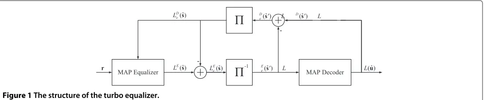
Figure 1 shows the structure of the turbo equalizer. The MAP equalizer takes as input the ISI-corrupted received symbols rand the extrinsic information LDe(sˆ) and pro-duces a sequence of posterior transmitted symbol log-likelihood ratio (LLR) estimatesLE(ˆs)(note thatLDe(sˆ)is zero during the first iteration). Extrinsic informationLEe(ˆs)
is determined by
LEesˆ=LEsˆ−LDe ˆs, (1)
which is deinterleaved to produce LEe(ˆs), which is used as input to the MAP decoder to produce a sequence of posterior coded symbol LLR estimates LD(sˆ). LD(ˆs)
is used together with LE
e(sˆ) to determine the extrinsic
information
LDe ˆs=LDsˆ−LEeˆs, (2)
LD
e(ˆs) is interleaved to produce LDe(sˆ). LDe(sˆ) is used
together with the received symbolsrin the MAP equal-izer, withLDe(sˆ) serving to provide prior information on the received symbols. The equalizer again produces pos-terior informationLE(ˆs)of the interleaved coded symbols. This process continues until the outputs of the decoder settle, or until a predefined stop-criterion is met [3]. After termination, the output L(uˆ) of the decoder gives an estimate of the source symbols.
Figure 1The structure of the turbo equalizer.
correlation between prior information and output infor-mation is minimized, allowing the system to converge to an optimal state in the solution space [4,5]. If informa-tion is exchanged directly between the equalizer and the decoder by ignoring interleaving and/or extrinsic infor-mation, self-feedback loops will be formed. This will cause minimal performance gains, since the equalizer and the decoder will inform each other about information already attained in previous iterations [4].
3 Modeling a turbo equalizer as a quasi-DAG Suppose a wireless communication system generates a column vector of source bits s of length Nu and s is
encoded by a convolutional encoder of rate Rc = 1/n,
producing a coded bit sequencecof lengthNc = Nu/Rc.
Now suppose that the coded bits sequence is interleaved using a random interleaver, which produces a bit sequence ´cof lengthNc, which is transmitted. The resulting symbol
sequence to be transmitted is given by
´
c=JGTs, (3)
where T denotes the transpose operation and G is an Nu×Ncmatrix
⎡ ⎢ ⎢ ⎢ ⎢ ⎢ ⎢ ⎢ ⎢ ⎢ ⎢ ⎢ ⎢ ⎢ ⎢ ⎢ ⎢ ⎢ ⎢ ⎣
g1K . . . gnK 0 . . . 0 0 0 0
..
. . .. ... g1K . . . 0 0 0 0
g11 . . . gn1 ... . . . 0 0 0 0
0 0 0 g11 . . . 0 0 0 0
..
. ... ... ... . .. ... ... ... ...
0 0 0 0 . . . gnK 0 0 0
0 0 0 0 . . . ... g1K . . . gnK
0 0 0 0 . . . gn1 ... . .. ...
0 0 0 0 0 0 g11 . . . gn1
⎤ ⎥ ⎥ ⎥ ⎥ ⎥ ⎥ ⎥ ⎥ ⎥ ⎥ ⎥ ⎥ ⎥ ⎥ ⎥ ⎥ ⎥ ⎥ ⎦ (4)
representing the convolutional encoder, where
g= ⎡ ⎢ ⎢ ⎣
g11 . . . gn1 ..
. . .. ...
g1K . . . gnK ⎤ ⎥ ⎥
⎦ (5)
is the generator matrix of a rate Rc = k/n (k = 1)
convolutional encoder with constraint length K andJis theNc×Ncinterleaver matrix. Now suppose the symbol
sequence´cis transmitted over a single-carrier frequency-selective Rayleigh fading channel with a time-invariant IR hof lengthL, the received symbol sequence is given by
r=Hc´+n, (6)
whereHis theNc×Ncchannel matrix with the channel
IRh= {h0, h1, . . ., hL−1}on the diagonal such that
H= ⎡ ⎢ ⎢ ⎢ ⎢ ⎢ ⎢ ⎢ ⎢ ⎢ ⎢ ⎢ ⎢ ⎢ ⎣
h0 0 . . . 0 0 0 0
..
. h0 . . . 0 0 0 0
hL−1 ... . .. 0 0 0 0
0 hL−1 . .. ... 0 0 0 ..
. ... . .. ... h0 0 0
0 0 0 hL−1 . . . h0 0
0 0 0 0 hL−1 . . . h0
⎤ ⎥ ⎥ ⎥ ⎥ ⎥ ⎥ ⎥ ⎥ ⎥ ⎥ ⎥ ⎥ ⎥ ⎦ (7)
andnis a complex Gaussian noise vector with 2Nc
sam-ples (Ncfor real andNcfor imaginary) from the
distribu-tionN(0,σ2).
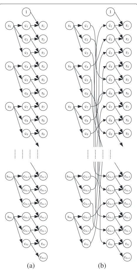
Figure 2a shows a graphical model of the transmission model in (6), without noise, where it is assumed thatJ=I whereIis anNc×Ncidentity matrix (i.e., no interleaving is performed) whereRc = 1/3 andL = 2. It shows that every uncoded bitsk producesRc−1 = 3 coded bitsck, ck+1andck+2, wherek=((k−1)/Rc)+1 (kruns from
1 toNu andkruns from 1 toNc). Each received symbol
can be expressed as
rk = L−1
l=0
ck−lhl, (8)
(b)
(a)
Figure 2Graphical models of (6) without (a) and with (b) a random interleaver.
a relationship between consecutive codewords (groups of
n bits). Figure 2a also depicts the causality relationship between the hidden variables and the observed variables.
Now consider Figure 2b. It shows a graphical model of the transmission model in (6), again without noise, but nowJis a randomNc×Ncinterleaver matrix and again Rc = 1/3 and L = 2. Each received symbol can be
expressed as
rk = L−1
l=0 ´
ck−lhl, (9)
where ´ck is the kth interleaved symbol. It is clear from
Figure 2b that there is no obvious relationship between the observed variablesrand the hidden variablescand that the causality relationship in Figure 2a is destroyed due to the randomization effect of the interleaver. Moreover the relationship between consecutive codewords (groups ofnbits) is also destroyed. This problem can therefore no longer be modeled as a DAG and exact inference is in fact impossible [8].
Deinterleaving the received sequencerwill ensure that the one-to-one relationship between each element in r andcis restored, but only with respect to the first coef-ficient h0 of the IR h. If h0 is dominant and if h is sufficiently short, approximate inference is possible due to the negligible effect ofh1tohL−1onr, but this is not normally the case. In a wireless communication system, transmitting information through a realistic frequency-selective Rayleigh fading channel h0 cannot be guaran-teed to be dominant and the contribution ofh1 tohL−1 is not negligible, and therefore this approach will fail. This has been simulated and verified by the authors. Another viable alternative is to model the system as a loopy graph in order to perform approximate inference as in [12], but as stated before, exact inference is impos-sible [8-10] and full convergence is not guaranteed [13]. In loopy graphs, convergence is normally achieved after many iterations.
The proposed DBN-TE addresses this problem by mod-eling the turbo equalizer as a quasi-DAG by applying a
transformationto the ISI-corrupted received symbols, in order to ensure that there will always exist a dominant connection between the hidden variable (codeword sym-bols) and the observed variable (received symsym-bols) at a given time instant, and only weak connections between the observed variable at the current time instant and hid-den variables at past and future time instances. With this transformation the DBN-TE achieves full conver-gence and is able to perform near-optimal inference in a small number of iterations, in order to estimate the coded sequencec, and hence the uncoded sequences.
4 Theoretical considerations
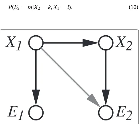
Consider a directed graph with (hidden) state variables
X1andX2, and observablesE1andE2(see Figure 3). We assume that these four random variables are binary.
As already mentioned, we assume that the observable variableE2 depends not only on the hidden variableX2, but also on the hidden variableX1. One way to get back to a classical hidden Markov chain problem is to com-bineX1andX2into “super nodes.” This increases the size of the state space and hence the computational complex-ity. We therefore use an iterative method instead, which is explained in Section 5.
We describe the iteration below, but first an infor-mal definition of the weak connection between hidden variable X1 and observed variable E2. For the current discussion, it is adequate to understand with a “weak con-nection” that the conditional probability distribution of the observed variableE2givenX2and{X1=0}is close to the distribution givenX2and{X1=1}. The answer to the question of how close these two conditional distributions have to be, can in principle be determined from the proof ofLemma1 below. Similar to the preceding section, our diagram is not a tree but a loopy DAG (or quasi-DAG).
To describe the iteration procedure, recall that for a hid-den Markov model, the event matrix at position(k,m)
is the probability that the observationm is made, given that the value of the hidden state isk. We will modify the forward–backward algorithm (described in Section 5.2.4) to compute the distribution of states given the evidence.
We now describe the iteration. Step 1 is to start with an initial estimate, say(i,j)of the states(X1,X2). Step 2 is to modify the forward–backward algorithm by modifying the event matrix that is used at time 2: change the entry in position(k,m)to
P(E2=m|X2=k,X1=i). (10)
X
1
X
2
E
2
E
1
Figure 3Non-Markovian DAG.We assume that the connection betweenX1andE2is “weak”.
Use the modified algorithm to compute the distribution of each state given the evidence. Find the most likely states from the distribution.
Step 2 can be iterated several times, but each time with the most recently obtained sequence of states in the place of the initial estimate(i,j). The claim is that these itera-tions will converge if the connection betweenE2andX1is “weak enough.”
In the rest of this section, we will interpret what “weak enough” means through notions of real analysis such as metric spaces and − δ description of continuity. The readers unfamiliar with these concepts can skip now to the next section without breaking the flow of their reading.
Note that we can put a metric (distance function) on the collection of event matrices, for example Euclidean distance will do.
The crux of the lemma is illustrated in Figure 4.
Lemma 1.Assume that at all iterations, the modified forward–backward estimates of the probabilitiesP(X1 = 1|E1=r,E2=s)andP(X2=1|E1=r,E2=s)are differ-ent from12and 0. Then, if the event matrices, correspond-ing to the different possibilities for the previous-iterate sequence of bits, are within sufficiently small distance of each other, the iteration procedure will converge to a fixed point; in fact the first and second iterations will already be identical.
11
00 10
01
ε
Proof. It is easy to show that for any fixed observation sequence(E1,E2)=(r,s)the dependence, of the posterior probability distribution of(X1,X2), on the choice of event matrices, is that of a continuous mapping. We can assume without loss of generality that the iteration is initialized at the state sequence(0, 0), because the argument below will apply to any initialization.
Let (p1,p2) be the modified forward–backward esti-mates obtained, for the probabilities P(X1 = 0,X2 = 0|E1 = r,E2 = s), when it is initialized at(0, 0). Because these estimates are assumed to be different from 12, the point(p1,p2)belongs to the interior of one of the quad-rants of the square [ 0, 1]×[ 0, 1]. Since it is in the interior, there is an > 0 so that the ball with midpoint(p1,p2) and radiusis contained in the same quadrant.
Our iteration procedure will now move to step 2 and initialize the modified forward–backward algorithm with the output of the first forward–backward run, which is the corner nearest to(p1,p2). Now, by the above-mentioned continuity of the posterior distribution on the used event matrices, there is aδ > 0 such that if the all the event matrices are within distanceδof the event matrix corre-sponding to the above-used initial guess (0, 0), then the output of the modified forward–backward algorithm will be within distance of (p1,p2). Therefore, it will be in the same quadrant as(p1,p2). So, rounding to the near-est corner will give the same corner as was yielded by the previous iteration.
We end this section by briefly discussing why this result can be expected to have a version that is also applicable to the less restrictive setup of the previous and next sections.
• More than two state variables: With a number of state variablesn, the square in the proof will become a hypercube inn dimensions, with2ncorners, each corner representing a possible previous sequence of estimates of each of then state variables. The proof will carry over; the−δdescription of continuous mappings is still applicable without
modification.
• Event matrices not “close enough:” If the first estimate of the hidden states is good, it is likely that it will be mapped to a quadrant, of which the corner will be mapped to the right quadrant in the next iteration. In this case more than one iteration will be needed. • More weak connections: With more than two state variables, it becomes possible thatEkis connected withXlfor somel<k−1.The entries of the event tables will then have to be set to a probability that is conditioned on a sequence longer than that appearing in equation (10). This does not affect the proof, as long as the connections are weak enough. Here the connections being weak enough means that the event matrices that are possible due to different
possible observation histories, are all close enough in the sense of the lemma.
5 DBN turbo equalizer
In this section, the DBN-TE is discussed. The first part explains the transformation that is applied to the chan-nel matrix in order to ensure that there exists a dominant connection between the observed variables and their cor-responding hidden variables, and the second part explains the operation of the DBN-TE, which jointly models the equalization and decoding stages on a quasi-DAG as defined in the previous section.
5.1 Transformation
For this exposition, assume that the coded symbolscare transmitted through a channelQ = HJ, whereHis the channel matrix andJis the interleaver matrix as previously defined. Therefore, Equation (6) can be written as
r=Qc+n. (11)
For the DBN-TE to perform approximate inference there must exist a strong connection between the observed variable and the hidden variable at time instance
k, and weak connections must exist between the observed variable at time instancekand hidden variables at other time instances. The randomization effect of the inter-leaver must also be mitigated in order for the turbo equal-izer to be modeled as a quasi-DAG so that there can exist a one-to-one relationship (dominant connection) between the observed variable and the corresponding hidden vari-able at time instancek.
To ensure that the connections between the observed variable and neighboring hidden variables are weak, the energy must be concentrated in the first taphoofh. This
can be achieved by applying a minimum phase prefilter to the received symbols r[14]. This process produces a filtered received symbol sequence and a minimum phase channel IR.
In order to model the turbo equalization problem as a quasi-DAG, the randomization effect of the random inter-leaver must be mitigated. Figures 5 and 6 showQfor systems with a channel IR lengths ofL = 1 andL = 3, respectively, for a hypothetical system with parameters
Nu = 50, Nc = 150, Rc = 1/3 at a mobile speed of 3 km/h and no frequency hops. It should be clear that any sequence c that is transmitted through a channelQ, as described in (11), will be subject to randomization.
To mitigate the effect of the interleaver, the following transformation is applied tor:
0
50
100
150
0 50
100 150
0 0.5 1 1.5
||Q||
Figure 5Qfor a system withL=1IR coefficients.
which is equivalent to transmitting the coded symbol sequencecthrough a channelU, where
U=QHQ, (13)
so that
QHr=Uc+QHn. (14)
Figures 7 and 8 show U for systems with channel IR lengths of L = 1 and L = 3, respectively. It is clear that this transformation mitigates the randomness exhibited in Q, since the new “channel” U is diago-nally dominant. The one-to-one relationship between the
observed variables and the corresponding hidden vari-ables are therefore restored. Minimum-phase filtering ofr is performed before performing the transformation in (12).
Therefore, applying a minimum-phase filter to r and performing the transformation in (14), all the conditions are met to model the turbo equalizer as a quasi-DAG with dominant connections between the observed variables and their corresponding hidden variables. Minimum-phase filtering ensures that a dominant connection exists between the observed variable and the hidden variable at time instancet, and that there exist weak connections
0
50
100
150
0 50
100 150
0 0.2 0.4 0.6 0.8 1
||Q||
0
50
100
150
0 50
100 150
0 0.5 1 1.5
||U||
Figure 7Ufor a system withL=1IR coefficients.
between the observed variable at time instance t and the hidden variable at other time instances, while the transformation in (14) mitigates the randomization effect of the interleaver so that there exists a one-to-one relationship between each observed variable and its corresponding hidden variable. By performing the trans-formation described here, all conditions for convergence as described in Section 4 are met.
5.2 The DBN-TE algorithm
After making preparation for the turbo equalization prob-lem to be modeled as a quasi-DAG, as explained in
the previous section, the DBN-TE algorithm can be executed. In this section, various aspects of the DBN-TE are discussed after which a step-by-step summary is provided in Section 5.2.8 in the form of a pseu-docode algorithm, encapsulating the working of the DNB-TE.
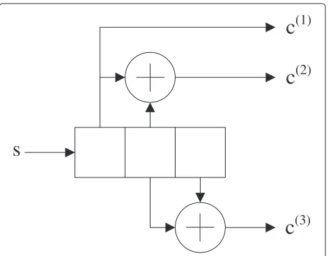
We assume a system with a uncoded block length ofNu, using the rateRc = 1/3, constraint lengthK = 3, con-volutional encoder in Figure 9 to produceNcbits, where
Nc = Nu/Rc. The coded bits are interleaved with a ran-dom interleaver and passes through a multipath channel with an IR of lengthL.
0
50
100
150
0 50
100 150
0 0.2 0.4 0.6 0.8 1
||U||
c
(1)c
(2)c
(3)s
Figure 9RateRc=1/3convolutional encoder.
5.2.1 Graph construction
The graph is constructed to model the possible outputs of a convolutional encoder in much the same way as a trel-lis is constructed in a conventional MAP decoder. For the DBN-TE graph the number of states per time instancetis equal to the number of possiblestate transitions, given by
M = 2K, whereK is the encoder constraint length. This is different from the number of states in a MAP decoder, which is equal to the number of possiblestates, given by
M=2K−1. The number of time instances in the DBN-TE graph is equal to the number of uncoded bitsNu, which
is also equal to the number of codewords. Figure 10a,b shows the graphical model of a DBN-TE for the first and subsequent iterations, respectively, where the dashed lines in Figure 10b depict weak connections due to ISI. Each Xton the graph contains a set ofMstate transitionsx(m)t ,
wheret=1, 2,. . .,Nuandm=1, 2,. . .,M.
During the first iteration no coded bit estimatesc˜ are available, so the graphical model is a pure DAG due to the fact that the current state is only dependent on the previous state. Hence onlyUt,t is used in the cost
func-tion of the sensor model, where Ut,t is a coefficient on
the diagonal of the new channel matrixUin (14). After the first iteration estimates of the coded bits c˜ are pro-duced and can therefore be used in subsequent iterations. During subsequent iterations then,Ut,u andUt,vare also
considered in the cost function of the sensor model, where
u=1, 2,. . .,t−1 andv=t+1,t+2,. . .,Nu.
5.2.2 State transition output table
The output associated with each state transition is also tabulated using the encoder state diagram in Figure 11. The output produced by each state transitionx(m)t ,m =
1, 2,. . ., 8, is determined by loading the bit-values of the current state into the leftmostK−1=2 fields of the con-volutional encoder in Figure 9, and then placing a 0 and a
X
1X
2X
3X
4X
N-1X
NX
1X
2X
3X
4X
N-1X
N(a)
(b)
01 00
10 11
xt
(1)
xt
(2)
xt(3)
xt(4)
xt(5)
xt(6)
xt(7)
xt
(8)
Figure 11Convolutional encoder state diagram.
1, respectively, on the input of the encoder, each produc-ing a new codewordc(1)c(2)c(3)at the output. This process
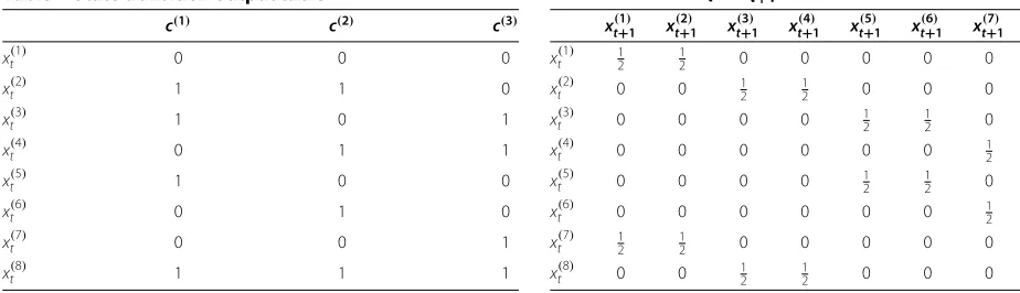
is followed exhaustively and tabulated. Table 1 shows the state transition outputs of the encoder in Figure 9 that results from moving from one state to the next.
5.2.3 Transition probability table
The DBN-TE depends on a transition model to describe the permissible state transitions. This is constructed by examining the encoder state transition diagram in Figure 11 and noting the possible state transitions. The solid lines and dashed lines indicate state transitions caused by ones and zeros at the input of the encoder. It is clear from Figure 11 that only two state transitions emanate from any given state transition (one caused by a 1 at the input and one caused by a 0 at the input). Table 2 shows the transition probabilities of the encoder in Figure 9 of which the state transition diagram is shown in Figure 11.
Table 1 State transition output table
c(1) c(2) c(3)
x(t1) 0 0 0
x(t2) 1 1 0
x(t3) 1 0 1
x(t4) 0 1 1
x(t5) 1 0 0
x(t6) 0 1 0
x(t7) 0 0 1
x(t8) 1 1 1
5.2.4 The forward–backward algorithm
The forward–backward algorithm computes the distribu-tion over past states given evidence up to the present [15]. It determines the exact MAP distribution P(Xk|e1:t)for
1 ≤ k <t, wheree1:tis a sequence of observed variables
from time 1 tot. This is done by calculating two evidence “messages”—the forward message from 1 up tokand the backward message fromk+1 up tot.
Forward message The forward message computes the posterior distribution over the future state, given all evi-dence up the current state. To compute the forward mes-sage, the current state is projected forward from timetto timet+1 and is then updated using the new evidenceet+1. To obtain the prediction of the next state it is necessary to condition on the current stateXt, hence:
P(Xt+1|e1:t+1)=αP(et+1|Xt+1)
xt
P(Xt+1|xt)P(xt|e1:t)
(15)
where α is a normalization constant, P(et+1|Xt+1) is obtained from the sensor model,P(Xt+1|xt)is the
transi-tion model andP(xt|e1:t)is the current state distribution.
The forward message can be computed recursively using (15).
Backward message The backwards message is computed in a similar fashion. It computes the posterior distribu-tion over past state, given all future evidence up to the current state. Whereas the forward message is computed forwards from 1 tok, the backwards message is computed backwards fromttok+1. Thus, the backwards message determines
P(ek+1:t|Xk)=
xk+1
P(ek+1|xk+1)P(xk+1|Xk)P(ek+2:t|xk+1)
(16)
Table 2 Transition probability table; transition probability table showingP(x(tm)|xt(+1n))
xt+(1)1 x(t+2)1 x(t+3)1 xt+(4)1 x(t+5)1 x(t+6)1 xt+(7)1 xt+(8)1
x(t1) 12 12 0 0 0 0 0 0
x(t2) 0 0 1
2 12 0 0 0 0
x(t3) 0 0 0 0 1
2 12 0 0
x(t4) 0 0 0 0 0 0 1
2 12
x(t5) 0 0 0 0 12 12 0 0
x(t6) 0 0 0 0 0 0 12 12
x(t7) 12 12 0 0 0 0 0 0
1 1.5 2 2.5 3 3.5 4 4.5 5 0.1
0.2 0.3 0.4 0.5 0.6 0.7 0.8 0.9 1
i
β
(i)
Figure 12The output of functionβ(i)forZ=3,Z=4 andZ=5 iterations.Blue diamond,Z=3; Blue square,Z=4; Blue circle,Z=5.
2 4 6 8 10 12 14 16 18 20
101 102 103 104 105 106 107 108 109
Channel IR length [L]
Normalized number of computations
where P(ek+1|xk+1) is obtained from the sensor model,
P(xk+1|Xk) is the transition model andP(ek+2:t|xk+1)is the current state distribution. The backward message can be computed recursively using (16).
Forward–backward message Finally, by combining the forward and backward message, the posterior distribution over all states at any time instance 1 ≤ k < tcan be determined as
P(Xk|e1:t)=αP(Xk|e1:k)P(ek+1:t|Xk). (17)
5.2.5 Sensor model
The conditional probabilities obtained from the sensor model for the respective forward and backward messages, P(et+1|Xt+1) and P(ek+1|xk+1) are determined by cal-culating a metric between the observed variable et and
the hidden variable x(m)t , where m = 1, 2,. . .,M. The observed variable et consists of Rc−1 received symbols rt+1tort+Rc−1, wheret
=((t−1)/Rc)+1 (truns from
1 toNuandtruns from 1 toNc), and the hidden variable
x(m)t consists of the output (c(1),c(2), andc(3)) associated with state transitionx(m)t in Table 1.
During the first iteration, only the dominant connec-tionUt,tbetween the observed variableetand the hidden
variablextis used in the cost calculation, since no coded
bit estimatesc˜are available at that point. Recall thatUis the new channel matrix brought about by performing the transformation in (12), resulting in the new transmission model in (14) having the desired properties to model the system as a quasi-DAG. During the first iteration the sys-tem can therefore be modeled as a pure DAG, as if no ISI occurred. Given a hidden variable or state transition out-putxnt+1, its associated bits (as tabulated in Table 1) are used together with observed variables/received symbols
rt+1tort+Rc−1, wheret
= ((t−1)/R
c)+1 andRc−1is
the number of encoder output bits, to calculate the cost of thenth state transition at time instancet
nt = R−1−1
j=0
rt+j−Ut+j,t+jcjn+1β(i)2, (18)
wheret=1, 2,. . .,Nuruns over time for the uncoded bit
estimates andβ(.)is a function that produces an optimiza-tion scaling factor for each iteraoptimiza-tioni.P(et+1|Xt+1)in (15)
0 1 2 3 4 5 6 7 8
10−4 10−3 10−2 10−1 100
Eb/No [dB]
BER
is determined by
P(et+1|xnt+1)=αexp(−nt/2σ2) (19)
where α is a normalization constant and σ is the noise standard deviation.
During subsequent iterations, LLR estimates of the uncoded bits are available, since the first set of LLRs are produced after the first iteration. Therefore, the system can be modeled as a quasi-DAG due to the fact that there exists a dominant connection between the observed vari-ableet and the hidden variablextand weak connections
between the observed variableet and other hidden
vari-ables. Thus we also use the rest of the coefficientsUt,1to Ut,Nc(and not onlyUt,t) in the cost calculation. Analo-gous to the first iteration, the output bits associated with a given state transitionxnt+1are used together with observed variablesrt+1 tort+Rc−1 as well asthe LLR estimatesc˜ of the uncoded bits to calculate the cost of thenth state transition at time instancet. Therefore, the cost of thenth state transition for subsequent iterations at time instance
tis given by
nt = Rc−1+1
j=0
rt+j−Ut+j,t+jcjn+1
−
Nc
v=1,v=t,Ut+j,v>0
Ut+j,v˜cvβ(i)2.
(20)
The last term in (20) contains the ISI terms that must be subtracted from the received symbols in order to minimizent so thatP(et+1|xnt+1), determined as in (19) can be maximized.
5.2.6 Computing LLR estimates
After the forward and backward messages are combined as in (17), the LLRs for each uncoded bit is determined from the graph. Rc−1 LLR vectors of length Nu are determined—each one corresponding to one output bit of the encoder—after which they are multiplexed to form one vector of lengthNc containing the LLR estimatesc˜
of the coded bits c. With reference to the state transi-tions in Table 1, the LLRs for the convolutional encoder in Figure 9, are determined as follows:
˜
c(1)=log
M
j=1,c(1)=1P(Xk|e1:t)
M
j=1,c(1)=0P(Xk|e1:t)
(21)
˜
c(2)=log
M
j=1,c(2)=1P(Xk|e1:t)
M
j=1,c(2)=0P(Xk|e1:t)
(22)
˜
c(3)=log
M
j=1,c(3)=1P(Xk|e1:t)
M
j=1,c(3)=0P(Xk|e1:t)
(23)
0 1 2 3 4 5 6 7 8
10−4 10−3 10−2 10−1 100
Eb/No [dB]
BER
The final LLR vector is constructed by multiplexing the respective LLR vectors such that
˜
c= {˜c(11),˜c(12),c1(3),˜c(21),c˜(22),c˜(23),. . .,c˜(N1u),c˜(N2u),˜c(N3u)} (24)
which is used in (20) in the next DBN-TE iteration.
5.2.7 Optimization
To improve the BER performance of the system, simu-lated annealing is used [15]. Simusimu-lated annealing is usually used in neural networks to allow the network to escape suboptimal basins of attraction in order to converge to a near-optimal solution in the solution space. Since the DBN-TE employs a soft-feedback mechanism, simulated annealing can also be applied to the coded symbol esti-mates c˜ that are fed back after the first iteration, thus allowing the DBN-TE to converge to a state where the BER performance is near-optimal. The optimization scaling functionβ(.)in (18) and (20)
β(i)=1.5(i−Z)/Z, (25)
whereZis the number of iterations, is updated with each iteration i, always starting at 0 < β(1) << 1 for the first iteration (i = 1) and finishing at β(Z) = 1 for the
final iteration (i = Z). Figure 12 showsβ(i)forZ = 3,
Z=4 andZ=5. Simulation results in Section 7 show the performance of the DBN-TE with and without simulated annealing.
5.2.8 Pseudocode algorithm
Additional file 1a–e shows the pseudocode of the DBN-TE algorithm. The DBN-TE algorithm iteratively computes the forward–backward message before producing LLR estimates of the coded symbols. After the final iteration the estimated turbo equalized uncoded information bits are returned.
Function definitions DBN TE receives as input the received ISI-corrupted coded symbols, the transition probability table, the transition output table, the code-word length, the coded data block length, the number of states of the graph, the new channel after transformation, the number of iterations and the noise standard deviation. FORWARD MESSAGE and BACKWARD MESSAGE receive as input the same variable as DBN TE, accept for the number of iterationsZ, and additionally they also received the LLR estimates and the optimization scaling factor as input.
0 1 2 3 4 5 6 7 8
10−4 10−3 10−2 10−1 100
Eb/No [dB]
BER
FORWARD BACKWARD MESSAGE receives only the result of FORWARD MESSAGE and BACK-WARD MESSAGE, while LLR ESTIMATES takes as input the forward–backward message resulting from FORWARD BACKWARD MESSAGE as well as the state transition output table.
Optimization scaling factor For each iteration a new optimization scaling factor is produced, as explained ear-lier. BETA implements (25) and returns the scaling factor used in the calculation of the forward and backward messages.
Forward message The algorithm starts by initializing the forward message, based on the initial state of the encoder shift register. Since it is assumed that the encoder shift register always starts in the all-zero state, the forward message is initialized accordingly, using the appropriate entries in the transition probability table (Table 2). The forward message is therefore initialized as
forward(1, :)=trans prob table(1, :), (26)
such thatforward(1, :)=[ 0.5, 0.5, 0, 0, 0, 0, 0, 0]since only state transitions x(t1+)1 and x(t2+)1 can emanate from state
transitionsx(t1) andx(t7), which lead to the all-zero state (see Figure 11).
The forward message is calculated next by iterating over time fromk = 2 tok = N while iterating overMstates
m = 1 tom = Mfor eachk. For each(k,m) pair, the forward message is initialized to zero, after which the mes-sage is updated by multiplying and accumulating mesmes-sages from the previous time-step k − 1. The forward mes-sages from the previous time-step k− 1 are multiplied with their respective transition probabilities (determined by the current state m) and summed together to form the new forward message at time-step k (at state m in the graph). Up to this point the forward message con-tains the collective contribution of the state distributions of the previous states, corresponding to the terms inside the summation in (15).
To include the evidence at graph state(k,m), the cost of the state transition associated with statemin the graph at timekmust be calculated. The GET COST functions takes as input the received codeword, LLR estimates of the codeword, the new channelU, the optimization scaling factor and the noise standard deviation, and determines the cost as in (18) for the first iterations and (20) for subsequent iterations. The forward message is updated
0 1 2 3 4 5 6 7 8
10−4 10−3 10−2 10−1 100
Eb/No [dB]
BER
by multiplying with the output of the normal probabil-ity distribution function NORMAL PDF (implemented as in (19)) which takes the cost and noise standard devi-ation as input. This completes the forward message. It now fully corresponds to (15). After computingMforward messages at time-stepk(one for each of theMstates at time-stepk), all the messages at time-stepkare normal-ized (NORMALIZE) so as to prevent message values from becoming very small due to multiplication of probabilities, when large data block sizes are used.
Backward message The backward message is initialized similar to the forward message, based on the final state of the encoder. The encoder is forced into the all-zero state and the end of the transmitted data block, and hence the backward message is initialized as
backward(N, :)=trans prob table(:, 1), (27)
such that backward(N, :) =[ 0.5, 0, 0, 0, 0, 0, 0.5, 0] since the state transitions emanating from the all-zero state,
xt(1+)1andx(t+2)1, are preceded by state transitions x(t1) and
x(t7).
The backward message is calculated in a similar fash-ion as the forward message, accept that iteratfash-ion over time
starts atk= N−1 and ends atk=1. Also note that the cost is not calculated for the current graph state(k,m), but for all those preceding it (at timek+1). Note the sensor model output isinsidethe summation in (16), whereas it is outside the summation in (15). The backward message is therefore calculated by accumulating information at the current graph state (at timek) from preceding graph states (at timek+1). The sensor model in (19) is applied (NOR-MAL PDF) to each preceding state, multiplied with the transition probability connecting the current state with the preceding state, and then multiplied with the message that corresponds to the preceding state. This result is then summed together for allMpreceding states and stored at the current state.
Forward–backward message The forward backward message is created by multiplying each corresponding for-ward and backfor-ward message value for each(k,m)pair, and normalizing the results as before.
Calculate LLR estimates The LLR estimates are calcu-lated in three phase to produce a sequence of N LLR estimates for each output bit of the decoder (assuming the rateRc = 1/3 convolutional encoder in Figure 9), after
0 1 2 3 4 5 6 7 8
10−4 10−3 10−2 10−1 100
Eb/No [dB]
BER
which the three LLR sequences are multiplexed to create a sequence of LLR estimates of lengthN/Rc. The LLR vec-tors are calculated by noting the ones and zeros in Table 1 that correspond to the respective output bits generated by the encoder. For instance, the first output bitc(1)in Table 1
is one for state transitionsx(t2),x(t3),x(t5)andx(t8), and zero forx(t1),x(t4),x(t6)andx(t7). The first LLR vector can there-fore be calculated as in (21). The second and third LLR vectors are calculated in the same fashion as in (22) and (23). The GET LLR function calculates the three LLR vec-tors, after which these vectors are multiplexed in function MULTIPLEX. The LLR estimates are used in (20) during the next iteration.
Result The result of the DBN-TE algorithm is deter-mined after the final iteration wheni= Z, by transform-ing the LLR sequence correspondtransform-ing to the first output bit of the encoder, into a bit sequence. The first LLR vector is used because the encoder in Figure 9 is systematic.
6 Complexity analysis
The computational complexity of the DBN-TE and the conventional turbo equalizer (CTE) are presented in this
section. The complexity equations were derived by count-ing the number of computations needed to perform Turbo Equalization. The complexity of the DBN-TE was deter-mined as
CCDBN−TE=Z(2NcMd+3NcMdQ/Rc), (28)
whereZis the number of turbo iterations,Mdis the
num-ber of decoder states determined by 2K−1whereKis the encoder constraint length,Qis the number of interfering symbols which can be approximated byQ≈ 2L−1, and
Rcis the code rate. The approximation forQwas obtained
empirically by calculating the average number of inter-fering symbols in the new channelUin (13) for a given original channel lengthL, after the transformation in (12) is applied. The complexity of the CTE was determined as
CCCTE=Z(4NcMeL+4NuMd/Rc), (29)
whereMeis the number of equalizer states determined by 2L−1for BPSK modulation.
Figure 13 shows the computational complexity graphs of the DBN-TE and the CTE, normalized by the number of coded transmitted symbols, for channel IR lengths from
L = 1 to L = 20, for Z = 3 andZ = 5. Rc = 1/3, Nu = 400,Nu = 1200 andK = 3. From Figure 13 it can
0 1 2 3 4 5 6 7 8
10−4 10−3 10−2 10−1 100
Eb/No [dB]
BER
be seen that the computational complexity of the DBN-TE is much higher (10 times higher atL = 2) than that of the CTE for systems with channel IR lengths L < 6. However, asLincreases beyondL=6, the computational complexity of the DBN-TE becomes significantly less than that of the CTE. The DBN-TE is therefore a good candi-date for systems with channel IR lengthsL>6. Note that forL = 20 the complexity of the DBN-TE is four orders less than that of the CTE.
7 Simulation results
The DBN-TE was evaluated in a mobile fading environ-ment for BPSK modulation, where we used the Rayleigh fading simulator in [16] to generate uncorrelated fading vectors. Simulations were performed at varying mobile speeds and different channel IR lengths, where the energy in the channel was normalized such thath†h = 1. The channel IR was “estimated” by taking the mean of the respective fading vectors in order to get estimates for the channel IR coefficients, unless otherwise stated. The uncoded data block length was chosen to beNu = 400
and the coded data block length wasNc = 1200, where
the rateRc = 1/3 convolutional encoder with generator
polynomialsg1(x) = 1,g2(x) = 1+x,g3(x) = x+x2in Figure 9 was used. Frequency hopping was also employed to reduce the BER.
Figures 14 and 15 show the performance of the DBN-TE and the CTE for different mobile speeds through channels with channel IR lengths ofL= 6 andL= 8, respectively. The frequency was hopped eight times, once for every 150 transmitted symbols. The DBN-TE was simulated for
Z = 3 iterations while the CTE was simulated forZ = 5 iterations. From Figures 14 and 15 it can be seen that the performance of the DBN-TE is less than a decibel worse than that of the CTE for mobile speeds of 3 and 20 km/h, while the performance of the DBN-TE closely matches the performance of the CTE for a mobile speed of 50 km/h. For mobile speeds of 80 and 110 km/h the DBN-TE out-performs the CTE. However, this result is of little practical importance, as the performance of both turbo equalizers at 80 and 110 km/h is no longer acceptable.
Figures 16 and 17 show the performance of the DBN-TE and the CDBN-TE for a fixed mobile speed of 20 km/h but with varying numbers of frequency hops, through chan-nels with channel IR lengths of L = 6 and L = 8, respectively. From Figures 16 and 17 it can be seen
0 1 2 3 4 5 6 7 8
10−4 10−3 10−2 10−1 100
Eb/No [dB]
BER
that the performance of the DBN-TE is again worse by less than a decibel for zero, two, four, and eight frequency hops.
Figure 18 shows the performance of the DBN-TE for channel IR lengths ofL = 5,L = 10, andL = 20 at a mobile speed of 20 km/h using 8 frequency hops forZ=5 iterations. From Figure 18 it is clear that the DBN-TE is able to turbo equalize signals in systems with longer mem-ory, due to its low complexity. With reference to Figure 13, the number of computations required by the DBN-TE for
L= 10 toL= 20 is in the range 103.84−104.15, whereas the number of computations required by the CTE is in the range 105.01−108.32.
In Section 5.2.7, optimization via simulated anneal-ing was discussed. To demonstrate the effect of sim-ulated annealing in the DBN-TE, simulations were performed with and without annealing for a channel IR length of L = 6 at speeds of 20 and 50 km/h, while the frequency was hopped four times (once for every 300 transmitted symbols) using Z = 3 itera-tions. Figure 19 shows the performance of the DBN-TE with and without simulated annealing. It is clear that the application of simulated annealing aids in improving the performance of the DBN-TE, where improvements
of approximately 1 dB are achieved for the selected scenarios.
In order to demonstrate the speed of convergence of the DBN-TE, Figure 20 shows the performance of the DBN-TE for different numbers of iterations(Z), where the channel IR length isL = 5 at a mobile speed of 20 km/h using eight frequency hops. From Figure 20 it can be seen that there is no significant increase in performance for
Z>3. The DBN-TE therefore almost fully converges after only three iterations.
The simulation results in Figures 14, 15, 16, 17, 18, 19 and 20 were produced under the assumption that the channel state information (CSI) is known, or that at least the very best estimate thereof is available, due to the averaging of each uncorrelated fading vector as explained earlier. To evaluate the robustness of the DBN-TE with respect to CSI uncertainties, the channel was estimated with a least squares (LS) estimator, using various amounts of training symbols. Figure 21 shows the performance of the DBN-TE and the CTE for a channel IR length of
L = 6 at a mobile speed of 20 km/h using 8 frequency hops, for 4L, 6L, and 8L training symbols in each fre-quency hopped segment of the transmitted data block. From Figure 21 it can be seen that the performance of
0 1 2 3 4 5 6 7 8
10−4 10−3 10−2 10−1 100
Eb/No [dB]
BER
the DBN-TE degrades, along with that of the CTE, due to insufficient amounts of training symbols, causing an increase in channel estimation errors. Is clear that the DBN-TE is as resilient against channel estimation errors as the CTE, as its performance closely matches that of the CTE.
The results presented in this section are self-evident and show that the DBN-TE achieves acceptable performance compared to that of the CTE. There is a small degrada-tion in BER performance compared to that of the CTE for all simulation scenarios, while a significant computa-tional complexity reduction is achieved for systems with longer memory. The complexity of the DBN-TE is only linearly related to the number of channel IR coefficients, while the complexity of the CTE is exponentially related to the channel IR coefficients, allowing the DBN-TE to be applied to systems with longer channels. The fast con-vergence of the DBN-TE demonstrated in Figure 20 also adds to the complexity reduction, as full convergence is achieved after only three iterations.
8 Conclusion
In this article, we have proposed and motivated a turbo equalizer modeled on a DBN which uses belief propaga-tion via the forward–backward algorithm, together with a soft-feedback mechanism, to jointly equalize and decode the received signal in order to estimate the transmit-ted symbols. We have motivatransmit-ted theoretically that this approach guarantees full convergence under certain con-ditions and we have shown that the performance of the new DBN-TE closely matches that of the CTE, with and without perfect CSI knowledge. Its complexity is lin-ear in the coded data block length, exponential in the encoder constraint length, but only approximately linear in the channel memory length, which makes it an attrac-tive alternaattrac-tive for use in systems with highly dispersive channels.
Additional file
Additional file 1: DBN-TE Pseudocode algorithm.(a) DBN-TE function pseudocode. (b) FORWARD MESSAGE function pseudocode. (c) BACKWARD MESSAGE function pseudocode. (d)
FORWARD BACKWARD MESSAGE function pseudocode. (e) LLR ESTIMATES function pseudocode.
Competing interests
The authors declare that they have no competing interests.
Author details
1Department of Electrical, Electronic and Computer Engineering, University of
Pretoria, Pretoria 0002, South Africa.2School of Engineering, University of Tasmania, Hobart 7001, Australia.3Department of Mathematics and Applied
Mathematics, University of Pretoria, Pretoria 0002, South Africa.
Received: 9 November 2011 Accepted: 23 May 2012 Published: 9 July 2012
References
1. C Berrou, A Glavieux, P Thitimajshima, inIEEE International Conference on Communications. Near Shannon limit error-correction and decoding: turbo-codes (1), vol 2, Geneva, 1993, pp. 1064–1070
2. C Douillard, M Jezequel, C Berrou, A Picart, P Didier, A Glavieux, Iterative correction of intersymbol intereference: turbo-equalization, Eur. Trans. Teleommun.6, 507–511 (1995)
3. G Bauch, H Khorram, J Hagenauer, inProceedings of European Personal Mobile Communications Conference (EPMCC). Iterative equalization and decoding in mobile communication systems, vol 2, 1997, pp. 307–312 4. R Koetter, M Tuchler, A Singer, Turbo equalization, IEEE Signal Process.
Mag.21, 67–80 (2004)
5. R Koetter, M Tuchler, A Singer, Turbo equalization: principles and new results, IEEE Trans. Commun.50(5), 754–767 (2002)
6. R Lopes, J Barry, The soft feedback equalizer for turbo equalization of highly dispersive channels, IEEE Trans. Commun.54(5), 783–788 (2006) 7. D Mackay,Information Theory, Inference, and Learning Algorithms.
(Cambridge University Press, Cambridge, 2003)
8. N Friedman, D Koller,Probabilistic Graphical Models: Principles and Techniques. (MIT Press, Cambridge, 2009)
9. Y Weiss,Belief Propagation and Revision in Networks with Loops. (MIT Press, Cambridge, 1997)
10. Y Weiss, W Freeman, Correctness of belief propagation in Gaussian graphical models of arbitrary topology, Neural. Comput.13, 2173-2200 (2001)
11. J Proakis,Digital Communications, 4th edn. (McGraw-Hill, International Edition, New York, 2001)
12. MI Jordan, KP Murphy, Y Weiss, inProceedings of Conference on Uncertainty in Artificial Intelligence. Loopy belief propagation for approximate inference: an empirical study, vol 15, Stockholm, 1999, pp. 467–475 13. Y Weiss, Correctness of local probability propagation in graphical models
with loops, Neural Comput.12, 1–41 (2000)
14. W Gerstacker, F Obernosterer, R Meyer, J Huber, On prefilter computation for reduced-state equalization, IEEE Trans. Wirel Commun.
1(4), 793–800 (2002)
15. S Russell, P Norvig,Artificial Intelligence: A Modern Approach, 2nd edn. (Prentic Hall, NJ, 2003)
16. Y Zheng, C Xiao, “Improved models for the generation of multiple uncorrelated Rayleigh fading waveforms”, IEEE Commun Lett. 6, 256–258 (2002)
doi:10.1186/1687-6180-2012-136
Cite this article as:Myburghet al.:Reduced complexity turbo equalization using a dynamic Bayesian network.EURASIP Journal on Advances in Signal Processing20122012:136.
Submit your manuscript to a
journal and benefi t from:
7Convenient online submission 7Rigorous peer review
7Immediate publication on acceptance 7Open access: articles freely available online 7High visibility within the fi eld
7Retaining the copyright to your article