Methods for depth-map filtering in view-plus-depth 3D video representation

(1)

Sergey Smirnov, Atanas Gotchev

*

and Karen Egiazarian

Abstract

View-plus-depthis a scene representation format where each pixel of a color image or video frame is augmented by per-pixel depth represented as gray-scale image (map). In the representation, the quality of the depth map plays a crucial role as it determines the quality of the rendered views. Among the artifacts in the received depth map, the compression artifacts are usually most pronounced and considered most annoying. In this article, we study the problem of post-processing of depth maps degraded by improper estimation or by block-transform-based compression. A number of post-filtering methods are studied, modified and compared for their applicability to the task of depth map restoration and post-filtering. The methods range from simple and trivial Gaussian smoothing, to in-loop deblocking filter standardized in H.264 video coding standard, to more comprehensive methods which utilize structural and color information from the accompanying color image frame. The latter group contains our modification of the powerful local polynomial approximation, the popular bilateral filter, and an extension of it, originally suggested for depth super-resolution. We further modify this latter approach by

developing an efficient implementation of it. We present experimental results demonstrating high-quality filtered depth maps and offering practitioners options for highest-quality or better efficiency.

1 Introduction

View-plus-depthis a scene-representation format where

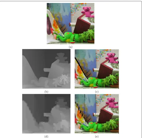
each pixel of the video frame is augmented with depth value corresponding to the same viewpoint [1]. The depth is encoded as gray-scale image in a linear or loga-rithmic scale of eight or more bits of resolution. An example is given in Figure 1a,b. The presence of depth allows generating virtual views through so-called depth image based rendering (DIBR) [2] and thus offers flex-ibility in the selection of viewpoint as illustrated in Fig-ure 1c. Since the depth is given explicitly, the scene representation can be rescaled and maintained as to address parallax issues of 3D displays of different sizes and pixel densities [3]. The representation also allows generating more than two virtual views which is demanded for auto-stereoscopic displays.

Another advantage of the representation is its back-ward compatibility with conventional single-view broad-casting formats. In particular, MPEG-2 transport stream standard used in DVB broadcasting allows transmitting auxiliary streams along with main video, which makes

possible to enrich a conventional digital video transmis-sion with depth information without hampering the compatibility with single-view receivers.

The major disadvantages of the format are the appear-ance of dis-occluded areas in rendered views and inabil-ity to properly represent most of the semi-transparent objects such as fog, smoke, glass-objects, thin fabrics, etc. The problems with occlusions are caused by the lack of information about what is behind a foreground object, when a new-perspective scene is synthesized. Such problems are tackled by occlusion filling [4] or by extending the format to multi-view multi-depth, or to

layered depth[3].

Quality is an important factor for the successful utili-zation of depth information. Depth map degraded by strong blocky artifacts usually produces visually unac-ceptable rendered views. For successive 3D video trans-mission, efficient depth post-filtering technique should be considered.

Filtering of depth maps has been addressed mainly from the point of view of increasing the resolution [5-7]. In [6], a joint bilateral filtering has been suggested to upsample low-resolution depth maps. The approach has been further refined in [7] by suggesting proper

anti-* Correspondence: [email protected]

Tampere University of Technology, Korkeakoulunkatu 10, FI-33720, Tampere, Finland

(2)

aliasing and complexity-efficient filters. In [5], a prob-abilistic framework has been suggested. For each pixel of the targeted high-resolution grid, several depth hypothesizes are built and the hypothesis with lowest cost is selected as a refined depth value. The procedure is run iteratively and bilateral filtering is employed at each iteration to refine the cost function used for com-paring the depth hypotheses.

In this article, we study the problem of post-proces-sing of depth maps degraded by improper estimation or

by block-transform-based compression. A number of post-filtering methods are studied, modified, and com-pared for their applicability to the task of depth map restoration and post-filtering. We consider methods ran-ging from simple and trivial smoothing and deblocking methods to more comprehensive methods which utilize structural and color information from the accompanying color image frame. The present study is an extension of the study reported in [8]. Some of the methods included in the comparative analysis in [8] have been further (a)

(b) (c)

(d) (e)

Figure 1Example of view-plus-depth image format and virtual view rendering (no occlusion filling applied for rendered images).(a)

True color channel;(b)true depth channel;(c)synthesized view using true depth;(d)highly compressed depth (H.264 I-frame with QP = 51);

(3)

2 Depth map characteristics 2.1 Properties of depth maps

Depth map is gray-scale image which encodes the dis-tance to the given scene pixels for a certain perspective. The depth is usually aligned with and ac-companies the color view of the same scene [9].

Single view plus depth is usually a more efficient representation of a 3D scene than two-channel stereo. It directly encodes geometrical information contained otherwise in the disparity between the two views thus providing scalability and possibility to render multiple views for displays with different sizes [1]. Structure-wise, the depth image is piecewise smooth (as representing gradual change of depth within objects) with delineated, sharp discontinuities at object boundaries. Normally, it contains no textures. This structure should be taken into account when designing compression or filtering algorithms.

Having a depth map given explicitly along with color texture, a virtual view for a desired camera position can be synthesized using DIBR [2]. The given depth map is first inversely-transformed to provide the absolute dis-tance and hence the world 3D coordinates of the scene points. These points are projected then onto a virtual camera plane to obtain a synthesized view. The techni-que can encounter problems with dis-occluded pixels, non-integer pixel shifts, and partly absent background textures, which problems have to be addressed in order to successfully apply it [1].

The quality of the depth image is a key factor for suc-cessful rendering of virtual views. Distortions in the depth channel may generate wrong objects contours or shapes in the rendered images (see, for example, Figure 1d,e) and consequently hamper the visual user experi-ence manifested in headache and eye-strain, caused by wrong contours of familiar objects. At the capture stage, depth maps might be not well aligned with the corre-sponding objects. Holes and wrongly estimated depth points (outliers) might also exist. At the compression stage, depth maps might suffer from blocky artifacts if compressed by contemporary methods such as H.264 [10]. When accompanying video sequences, the consis-tency of successive depth maps in the sequence is an issue. Time-inconsistent depth sequences might cause flickering in the synthesized views as well as other 3D-specific artifacts [11].

Depth quantization is normally done in linear or loga-rithmic scale. The latter approach allows better preser-vation of geometry details for closer objects, while higher geometry degradation is tolerated for objects at longer distances. This effect corresponds to the parallax-based human stereo-vision, where the binocular depth cue losses its importance for more distanced objects and is more important and dominant for closer objects. The same property can be achieved if transmitting linearly quantizedinversedepth maps. This type of depth repre-sentation basically corresponds tobinocular disparity

(also known as horizontal parallax), including again necessary modifications, such as scaling, shifting, and quantizing.

2.2 Depth map filtering problem formulation

This section formally formulates the problem of filtering of depth maps and specifies the notations used here-after. Consider an individual color video frame in YUV (YCbCr) or RGB color space y(x) = [yY(x),yU(x), yV(x)] or y(x) = [yR(x),yG(x),yB (x)], together with the asso-ciated per-pixel depthz(x), wherex= [x1,x2] is a spatial

variable,x ÎX, Xbeing the image domain.

A new, virtual viewh(x) = [hY(x),hU(x),hV(x)] can be synthesized out of the given (reference) color frame and depth by DIBR, applying projective geometry and knowledge about the reference view camera, as dis-cussed in Section 2.1 [2]. The synthesized view is com-posed of two parts, h=hv +ho, wherehv denotes the visible pixels from the position of the virtual view cam-era and ho denotes the pixels of occluded areas. The

corresponding domains are denoted byXvand Xo corre-spondingly,Xv⊂X,Xo=X\Xv.

Both y(x) and z(x) might be degraded. The degrada-tions are modeled as additive noise contaminating the original signal

yC_q =yC+εC, (1)

zq=z+∈, (2)

whereC=Y, U, V or R, G, B. Both degradations are modeled as independent white Gaussian processes:

εC₍_·₎_∼_N_(0,_σ2

C),ε(·)∼N(0,σ2). Note that the variance

of color signal noise (σ2

C) differs from the one of the

(4)

If degraded depth and reference view are used in DIBR, the result will be a lower-quality synthesized view

η. Unnatural discontinuities, e.g., blocking artifacts, in the degraded depth image cause geometrical distortions and distorted object boundaries in the rendered view. The goal of the filtering of degraded depth maps is to mitigate the degradation effects (caused by e.g., quanti-zation or imperfect depth estimation) in the depth image domain, i.e., to obtain a refined depth image esti-mate _ˆz, which would be closer to the original, error-free depth, and would improve the quality of the rendered view.

2.3 Depth map quality measures

Measuring the quality of depth maps has to take into account that depth maps are type of imagery which are not visualized per-se, but through rendered views.

In our study, we consider two types of measures:

•measures based on comparison between processed

and ground truth(reference) depth;

• measures based on comparison between virtual

views rendered from processed depth and from ground truth one.

Measures for the first group have the advantage of being simple, while measures from the second group are closer to subjective perception of depth. For both of these groups we suggest and test new measures.

PSNR of Restored Depth

Peak signal-to-noise ratio (PSNR) measures the ratio

between the maximum possible power of a signal (within its range) and the power of corrupting noise.

PSNR is commonly used as a measure of fidelity of

image reconstruction. PSNRis calculated via the mean squared error (MSE):

MSE= 1

N

x

(z(x)− ˆz(x))2, (3)

PSNR= 10log₁₀ MAX2 z MSE (4)

where z(x) and zˆ(x)are the reference and processed signals; Nis number of samples (pixels) and MAXzis the maximal possible pixel value, assuming the minimal one is zero. In this metric higher value means better

quality. ApplyingPSNRto depth images must be done

with care and with proper rescaling, as most of depth maps have a sub-range of the usual 8-bit range of 0 to 255 andPSNRmight turn to be unexpectedly high. PSNR of rendered view

PSNRis calculated to compare the quality of rendered view using processed depth versus that of using original

depth [10]. It essentially measures how close the ren-dered view is to the‘ideal’one. In our calculations, pix-els, dis-occluded during the rendering process, are excluded so to make the comparison independent on the particular hole fitting approach. For color images, we calculatePSNRindependently for each color channel and then calculate the mean between three channels. Percentage of bad pixels

Bad pixels percentage metric is defined in [12] to mea-sure directly the performance of stereo-matching algo-rithms.

BAD= 100

M

x

z(x)− ˆz(x)> d,

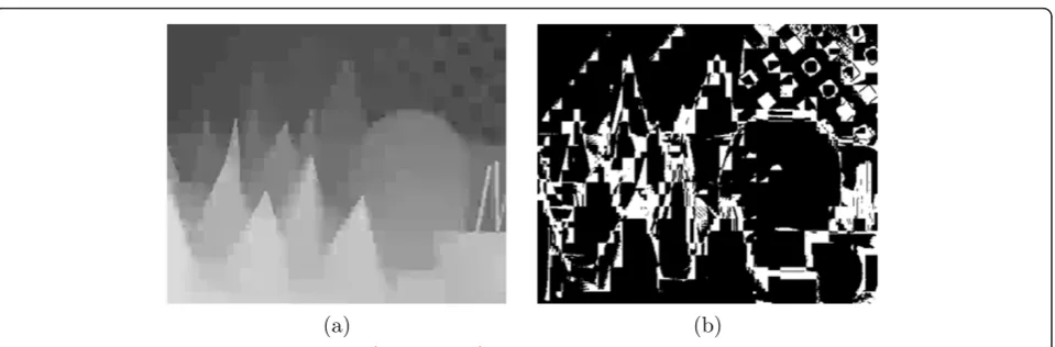
where z_ˆis the computed depth, z is the true depth andΔdis a threshold value, (usually equal to 1). Figure 2 shows thresholding results for some highly com-pressed depth maps. We include this metric to our experiments in an attempt to check its applicability for comparing post-filtering methods. For this metric, lower value means better quality.

Depth consistency

Analysing the BAD metric, one can notice that the

thresholding imposed there, does not emphasize the importance of small or big differences. It is equally important, when the error is just a quantum above the threshold and when it is quite high.

In a case of depth degraded by compression artifacts, almost all pixels are quantized thus changing their

origi-nal values and therefore causing the BAD metric to

show very low quality while the quality of the rendered views will not be that bad.

Starting from the idea that the perceptual quality of rendered view will depend more on the amount of geo-metrical distortions than on the number of bad depth pixels, we suggest to give preference to areas where the change between ground truth depth and compressed

depth is more abrupt. Such changes are expected to

cause perceptually high geometrical distortions.

Consider the gradient of the difference between true depth and approximated depth∇ξ =∇(z− ˆz). Bydepth

consistencywe denote the percentage of pixels, having

magnitude of that gradient higher than a pre-specified threshold.

CONSIST= 100

N

(∇ξ2> σconsist). (5)

The measure favors non-smooth areas in the restored depth considered as main source of geometrical distor-tion, as illustrated in Figure 3.

Gradient-Normalized RMSE

(5)

gradient-normalized RMSE metric. Such measure decreases the over-penalization of errors caused by fine textures.

In our implementation, we calculate this metric for the luminance channels of reference and rendered views and exclude occluded areas determined by the DIBR on the ground truth data.

NRMSE_η = ⎡

⎣

x∈Xv

ηY₍_x₎_{− ˆ}_ηY₍_x₎2 _∇ηY₍_x₎2_{+ 1}

⎤ ⎦

1/2

, (6)

wherehY(x) is the luminance of the virtual image gen-erated by ground truth depth and_η_ˆY

(x)is the luminance of virtual image generated by processed depth. For bet-ter quality, the metric shows low values.

Discontinuity Falses

We propose using a measure based on counting of wrong occlusions in the view rendered out of processed depth. If all occlusions between true and processed vir-tual images coincide, then depth discontinuities are pre-served correctly.

DISC= 100

N #

Xo∪ ˆXo

\Xo∩ ˆXo

, (7)

where #(X) is cardinality (number of elements) of a

domainX. The measure decreases with improving the

quality of the processed depth.

3 Depth filtering approaches

A number of post-processing approaches for restoration of natural images exist [14]. However, they are not directly applicable to range images due to differences in image structure.

In this section, we consider several existing filtering approaches and modify them for our need. First group of approaches works on the depth map images with using no structural information from the available color channel. Gaussian smoothing and H.264 in-loop deblocking filter [15] are the filtering approaches included in this group. The approaches of the second group actively use available color frame to improve depth map quality. While there is an apparent

(a) (b)

Figure 2BAD pixels mask for“Cones”datasetz(x)− ˆz(x)> dcaused by H.264 Intra compression with QP = 51.

(a) (b)

Figure 3Distortions in depth“Teddy”dataset (||∇ξ||2>sconsist) caused by H.264 Intra compression with (a) QP = 51 and the same

(6)

correlation between the color channel and the accompa-nying depth map, it is important to characterize which color and structure information can help for depth processing.

More specifically, we optimize state-of-the-art filtering

approaches, such as local polynomial approximation

(LPA) [16] and bilateral filtering [17] to utilize edge-pre-serving structural information from the color channel for refining the blocky depth maps. We suggest a new version of the LPA approach which, according to our experiments, is most appropriate for depth map filtering. In addition, we suggest an accelerated implementation of the method based on hypothesis filtering as in [5], which shows superior results for the price of high com-putational cost.

3.1 LPA approach

The anisotropic LPA is a pixel-wise method for adaptive signal estimation in noisy conditions [16]. For each pixel of the image, local sectorial neighborhood is con-structed. Sectors are fitted for different directions. In the simplest case, instead of sectors, 1D directional esti-mates of four (by 90 degrees) or eight (by 45 degrees) different directions can be used. The length of each sec-tor, denoted asscale, is adjusted to meet the compro-mise between the exact polynomial model (low bias) and sufficient smoothing (low variance). A statistical cri-terion, denoted as intersection of confidence intervals

(ICI) rule is used to find this compromise [18,19], i.e.,

the optimal scale for each direction. These optimal

scales in each direction determine an anisotropic star-shape neighborhood for every point of the image well adapted to the structure of the image. This neighbor-hood has been successfully utilized for shape-adaptive transform-based color image de-noising and de-blurring [14].

In the spirit of [14], we use the quantized luminance channelyY

q =yY+εY as source of structural information.

The image is convolved with a set of 1D directional polynomial kernelsghj,θk

, where{h}J_j₌₁is the set of dif-ferent lengths (scales) and θk=kπ

4,k= 1, 2,. . ., 8are

the directions, thus obtaining the estimates

yhj,θk(x) =

yY q ∗ghj,θk

(x). The ICI rule helps to find the optimal scaleh+(x) for each direction (the notation of

direction is omitted). This is the largest scale (in

num-ber of pixels), which ensures a non-empty ICI

[18,19]Ji=∩ji=1Iiwhere

Ii=

yhi(x)−σ

Y_g

hi,yhi(x) +σ

Y_g

hi. (8)

After finding optimal scales h+(x) for each direction at

pixel x0 a star shape neighborhood x0is formed, as

illustrated in Figure 4a. There is a clear evidence that there is a relation between the adaptive neighborhoods and the (distorted) depth, as examplified in Figure 4b. Adaptive neighborhoods are formed for every pixel in

the image domain X. Once adaptive neighborhoods are

found, one must find some modeling for depth channel before utilizing this structural information.

Constant depth model

For our initial implementation of LPA-ICI depth filter-ing scheme, the depth model is rather simple. The depth map is assumed to be constant in the neighbor-hood of the filtering pixel x0, where neighborhood is

found by the LPA-ICI procedure. This modeling is based on the assumption that the luminance channel is nearly planar at areas where the depth is smooth (close to constant). Whenever the depth has a nuity, the luminance is most likely to have a disconti-nuity too. The constant-modeling results in simple weighted average over the region of optimal neighbor-hood

∀x0,∃x0,zq(x)≈const,x∈x0, (9)

ˆ

z(x0) =

1

N

x∈x0

zq(x), ₍₁₀₎

whereNis the number of pixels inside adaptive

sup-portx0. Note, that the scheme depends on two

para-meters: the noise variance of the luminance channelsY and the positive threshold parameter Γ. The latter can be adjusted so to control the smoothing in restored depth map.

Linear regression depth model

In a more sophisticated approach we apply pixelwise-planar depth assumption, stating of pixelwise-planarity of depth inside some neighborhood of processing pixel. This is a higher order extension of the previous assumption.

∀x0,∃x0,zq(x)≈Ax˜,x˜= [x, 1],x∈x0, (11)

wherex_ˆis homogeneous coordinate.

Based on this assumption, instead of simple averaging in depth domain we apply plane fitting (linear regres-sion). A=dB-1, whered is a row-vector of depth values z(x),x∈x0,Bis a 3-by-N matrix of their homogeneous

coordinates in image space and B-1 is Moore-Penrose

pseudoinverse of rectangular matrix. Estimated depth values are found with a simple linear equation:

ˆ

z(x) =Ax˜,x˜= [x, 1],x∈x0. (12)

Aggregation procedure

(7)

ˆ

zagg(x0) =

1

M

j=1..M ˆ

zj(x0), ₍₁₃₎

whereMis number of estimates coming from overlap-ping regions in particular coordinate x0. A result of

depth, filtered by LPA-ICI is given in Figure 4e. Color-driven LPA-ICI

Luminance channel of the color image is usually consid-ered as the most informative channel for processing and also as the most distinguishable by the human visual system. That is why many image filtering mechanisms use color transformation to extract luminance and then process it in different way to compare with chrominance channels. This also may be explained by the fact that luminance is usually the less noisy component and thus it is most reliable. Nevertheless, for some color proces-sing tasks pixel differentiation based only on luminance channel is not appropriate due to some colors may have the same luminance whereas they have different visual appearance.

Our hypothesis is that a color difference signal will better differentiate color pixels, as illustrated in Figure

5. L2 norm is used to form a color difference map

around pixelx0:

Cx0_x =

(Yx0−Yx)2+ (Ux0−Ux)2+ (Vx0−Vx)2, (14)

wherex0is the currently processing pixel, and x∈x0.

The color difference map is used as a source of struc-tural information, i.e., the LPA-ICI procedure is run over this map instead over the luminance channel. Dif-ferences are illustrated in Figure 5. In our implementa-tion, we calculate color-difference only for those pixels of the neighborhood which participate in 1D directional convolutions. Additional computational cost of such implementation is about 10% of the overall LPA-ICI procedure.

For all mentioned LPA-ICI based strategies the main adjusting parameter, capable to set proper smoothing for varying depth degradation parameter (e.g., varying QP in coding) is the parameterΓ.

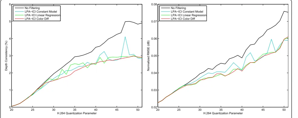
3.1.1 Comparison of LPA-ICI approaches The perfor-mance of different versions of the LPA-ICI approach are compared in Figure 6. The ‘normalized RMSE’(equation 6) and ‘depth consistency’ (equation 5) metrics have been computed and averaged over a set of test images. The parameters of the filters were empirically optimized with‘depth consistency’(equation 5) as a cost measure. As it can be seen, the color-driven LPA-ICI approach

(a) (b) (c)

(d) (e)

Figure 4Example of adaptive neighborhoods:(a)luminance channel with some of found optimal neighborhoods;(b)compressed depth with the same neighborhoods overlaid;(c)optimal scales for one of the direction (black for small scale and white for big scale);(d)example of

(8)

with plane fitting and encapsulated aggregation is the best performing approach, while also having the most stable and consistent results. Because of the superior performance of color-driven LPA-ICI, we use it in the

experiments from now on. All experiments and compar-isons involving LPA-ICI presented in the following sec-tions refer to the optimized color-driven LPA-ICI implementation.

(a) (b)

(c) (d)

Figure 5Example of different LPA-ICI implementations:(a)luminance channel;(b)color-difference channel for central pixel of a red square;

(c)LPA-ICI filtering result, optimal scales were found in luminance channel;(d)LPA-ICI filtering result, optimal scales were found in color-difference channel.

20 25 30 35 40 45 50 0

1 2 3 4 5 6

H.264 Quantization Parameter

Depth Consistency (%)

No Filtering LPA−ICI Constant Model LPA−ICI Linear Regression LPA−ICI Color Diff

20 25 30 35 40 45 50 0.02

0.03 0.04 0.05 0.06 0.07 0.08

Normalized RMSE (dB)

No Filtering LPA−ICI Constant Model LPA−ICI Linear Regression LPA−ICI Color Diff

(9)

near values to distant values in both spatial domain and range. For color images, bilateral filtering uses color dis-tance to distinguish photometric similarity between pix-els, which affects in reducing phantom colors in the resulting image. In our approach, we calculate filter weights using information from color frame in RGB, while applying filtering on depth map. Our design of bilateral filter has been inspired by [5], as follows:

ˆ

z(x) =

uωs(x−u) ωcy(x)−y(u)zq(u)

uωs(x−u) ωcy(x)−y(u)

, (15)

where

ωa(t) =e− t

γa_{, (}_a₌_s_,_c₎andu Î Ωx are neigh-borhood pixels of point x. This design allows for rela-tively fast implementation by storing all possible color and distance weights as look-up tables. Parametersgs,gc

and processing window size Ωx are adjustable

para-meters of the filter. Figure 7 illustrates the filtering. The color channel (Figure 7a) provides the color difference information, with respect to the processed pixel position (Figure 7b). It is further weighted by spatial Gaussian fil-ter to defil-termine the weights of pixels from the depth map taking part in estimating the current (central) pixel (Figure 7f).

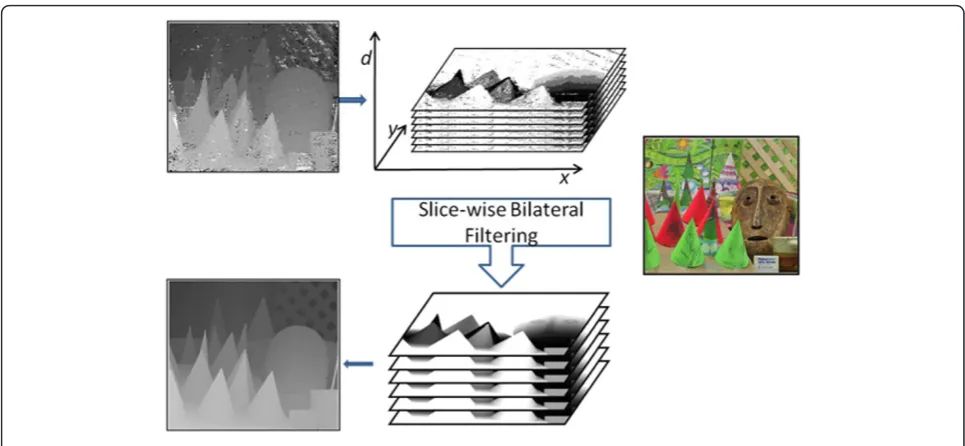
3.3 Spatial-depth super resolution approach

A post-processing approach was suggested aimed at increasing the resolution of low-resolution depth images, given high-resolution color image as a reference [5]. In our study, we study the applicability of this filter for suppression of compression artifacts and restoration of true discontinuities in the depth map. The main idea of the filter is to process depth in probabilistic manner, constructing 3D cost volume from several depths hypothesizes. After bilateral filtering of each slice of the volume, the hypothesis with the lowest cost is selected as a new depth value. The procedure is applied itera-tively, calculating cost volume using the depth estimated in previous step. The cost volume on ith iteration is constructed to be quadratic function of the current depth estimate:

C(i)(x,d) = min

L_η,d−z(i)(x)

2

, (16)

whereLhdenotes tunable search range.

obtained by winner-takes-all approach will be discrete as well. To tackle this effect, the final depth estimate is taken as the minimum point of quadratic polynomial which approximates the cost function between three dis-crete depth candidates:d, d- 1 andd+ 1

f(d) =ad2+bd+c, (17)

dmin=−

b

2a. (18)

f (dmin) is the minimum of quadratic function f(d), thus givend, f(d),f(d-1) and f(d +1), valuedmincan be calculated:

dmin=d−

f(d+ 1)−f(d−1)

2(f(d+ 1)−f(d−1)−2f(d). (19)

After the bilateral filtering is applied to the cost volume, the depth is refined and true depth discontinu-ities might be completely recovered.

In our implementation of the filter, we have suggested two simplifications:

•we use only one iteration of the filter;

•before processing we scale the depth range by fac-tor of 20, thus reducing the number of slices, and subsequently reducing the processing time.

The main tunable parameters of the filter are the parameters of the bilateral filter gdand gc. As long as the processing time of the filter still remains extremely high, we do not perform optimization of this filter directly, but assume that the optimal parametersgd=fd (QP) andgc =fc(QP) found for the direct bilateral filter are optimal or nearly optimal for this filter as well.

3.4 Practical implementation of the super resolution filtering

(10)

ˆ

z(i+1)(x) = arg min

d

u∈xW(x,u)G(u,d)

u∈xW(x,u)

,

W(x,u) =ωs(x−u) ωcy(x)−y(u),

G(u,d) = minη∗L,d−z(i)(u)

2

.

(20)

Furthermore, the computation cost is reduced by assuming that not all depth hypotheses are applicable for the current pixel. A safe assumption is that only depths within the rangedÎ [dmin, dmax] wheredmin=

min(z(u)),dmax= max(z(u)),uÎΩxhave to be checked. Additionally, depth range is scaled with the purpose to further reduce the number of hypothesizes. This step is

especially efficient for certain types of distortions such as compression (blocky) artifacts. For compressed depth maps, the depth range appears to be sparse due to the quantization effect.

Figure 10 illustrates histograms of depth values before and after compression so to confirm the use of rescaled search range of depth hypotheses. This modification speeds up the procedure and relies on the subsequent quadratic interpolation to find the true minimum. A pseudo-code of the suggested procedure in Equation 20 is given in following listing.

Require:C, the color image;D, the depth image;X, a spatial image domain

(a) (b)

(c) (d)

(e) (f)

Figure 7Example of bilateral filtering:(a)color channel;(b)color-difference for central pixel (marked red);(c)color-weighed component of

bilateral product;(d)complete weights for selected window ((c) multiplied with spatial Gaussian component);(e)example of blocky depth map

(11)

for allxÎX do

dmin= min

u∈x

Du,dmax= max

u∈x Du

ifdmax-dmin<gthrthen

ˆ

Dx=Dx

else

F(x,u) = Cu−Cx u−x

uCu−Cx u−x{bilateral weights}

Sbest ¬ Smax {Smaxis maximum reachable value

forS}

Figure 8Principle of super-resolution filtering.

(a) (b)

(c) (d)

(12)

ford=⌊dmin⌋to [dmax]do

S¬ 0

for alluÎΩxdo

E¬min{(d-Du)2,hL}

S¬S+F(x,u)*E

end for ifS<Sbestthen

Sbest¬S

dbest ¬d

end if end for

ˆ

Dx=dbest

end if end for

The memory foot-print required by our implementa-tion is significantly lower than the one imposed by a direct implementation. A straightforward implementa-tion would require a large memory buffer to store the complete cost volume in order to process it pixel-by-pixel and avoid computing (the same) color weights across different slices. In the proposed implementation, two memory buffers with relatively low sizes are required: a memory buffer which is equal to the proces-sing window size to store current color weights, and a buffer to store the cost values for the current pixel along the‘d’dimension. In case of multi-thread (paralle-lized) implementation, these memory buffers are multi-plied by the number of processing threads. More information about platform-specific optimization of the proposed algorithm is given in [20].

Figure 11 illustrates the performance in terms of speed. The figure shows experiments with different

implementations of the filtering procedure. The‘Teddy’ dataset has been processed (see also Figure 12 for refer-ence). All filter versions have been implemented in C and then compiled into MEX files to be run within Matlab environment. The experiments have been run on a 1.3 GHz Pentium Dual-Core processor with 1 Gb of RAM under MS Windows XP operating system. In the figure, the vertical axis shows the execution time in seconds and the horizontal line shows the number of slices processed (i.e., the depth dynamic range assumed). The dotted curve shows single-pass bilateral filtering. It does not depend on the dynamic range, but on the win-dow size, thus it is a constant in the figure. The red line shows the computational time for the original approach implemented as a three step procedure for the full dynamic range. Naturally, it is a linear function with respect to the slices to be filtered. Our implementation (blue curve) applying a reduced dynamic range is also linearly depending on the number of slices, but with dramatically reduced steepness.

4 Experimental results 4.1 Experimental setting

In our experiments, we consider depth maps degraded by compression. Thus degradation is characterized by the quantization parameter (QP). For better comparison of selected approaches, we present two types of experi-ments. In the first set of experiments, we compare the performance of all depth filtering algorithms assuming the true color channel is given (it has been also used in the optimization of the tunable parameters). This shows ideal filtering performance, while in practice it cannot

50 100 150 200

Depth range

Number of pixels

50 100 150 200

Depth range

Number of pixels

(a)

(b)

(13)

be achieved due to the fact that the color data is also degraded by e.g., compression.

In the second set of experiments, we compare the effect of depth filtering in the case of mild quantization of the color channel. General assumption is that color data is transmitted with backward compatibility in mind, and hence most of the bandwidth is occupied by the color channel. Depth maps in this scenario are heav-ily compressed, to consume not more than 10-20% of the total bit budget [21,22].

We consider the case where both y and z are to be

coded as H.264 intra frames with some QPs, which leads to their quantized versions yq andzq. The effect of quantization of DCT coefficients has been studied thor-oughly in the literature and corresponding models have been suggested [23]. Following the degradation model in Section 2.2, we assume quantization noise terms added to the color channels and the depth channel considered

as independent white Gaussian processes:

εC₍_·₎_∼_N_(0,_σ2

C),ε(·)∼N(0,σ2). While this modeling is

simple, it has proven quite effective for mitigating the blocking artifacts arising from quantization of transform coefficients [14]. In particular, it allows for establishing a direct link between the QP and the quantization noise

variance to be used for tuning deblocking filtering algo-rithms [14].

Training and test datasets for our experiments (see Figure 12) were taken from Middlebury Evaluation Test-bench [12,24,25]. In our case, we cannot tolerate holes and unknown areas in the depth datasets, since they produce fake discontinuities and unnatural artifacts after compression. We semi-manually processed 6 images to fill holes and to make their width and height be multi-ples of 16.

4.1.1 Parameters optimization

Each tested algorithm has a few tunable parameters which could be modified according particular filtering strategy related with a quality metric. So, to make com-parison as fair as possible, we need to tune each algo-rithm to its best, according such a strategy and within certain range of training data.

Our test approach is to find empirically optimal para-meters for each algorithm over a set of training images. It is done separately for each quality metric. Then, for each particular metric we evaluate it once more on the set of test images and then average. Then comparison

between algorithms is done for each metric

independently.

(14)

Particularly, for bilateral filtering and hypothesis (super-resolution) filtering we are optimizing the follow-ing parameters: processfollow-ing window size,gs andgc. For

the Gaussian Blurring we are optimizing parameterss

and processing window size. For LPA-ICI based approach we are optimizing theΓparameter.

4.2 Visual comparison results

Figures 13 and 14 present depth images paired with consecutive rendered frames (no occlusion filling is

applied). This approach helps to illustrate artifacts in the depth channel as well as their effect on the rendered images.

As it is seen in the top row (a), rendering with true depth, results in sharp and straight object contours, as well as in continuous shapes of occlusion holes. For such holes, a suitable occlusion filling approach will pro-duce good estimate.

Row (b) shows unprocessed depth after strong com-pression (H.264 with QP = 51) frame and its rendering

(15)

capability. Objects edges are particularly affected by block distortions.

With respect to occlusion filling, the methods behave as follows.

• Gaussian smoothing of depth images is able to

reduce number of occluded pixels, making occlusion filling simpler. Nevertheless, this type of filtering

does not recover geometrical properties of depth, which results in incorrect contours of the rendered images.

•Internal H.264 in-loop deblocking filtering was performed similarly to the Gaussian smoothing, with no improvement of geometrical properties.

•LPA-ICI based filtering technique performs signifi-cantly better both is sense of depth frame and (a)

(b)

(c)

(d)

Figure 13Visual results for_“Teddy_”dataset. Left column: depth, right column: respective rendered result (no occlusion filling applied).(a)

(16)

rendered frame visual quality. Geometrical distor-tions are less pronounced, however, still visible in rendered channel.

• Bilateral filter almost recovers the sharp edges in depth image, while has minor artifacts (for instance, see chimney of house).

• Super-resolution depth filter recovers discontinu-ities as good as bilateral or even better. Resulted depth image does not have artifacts as in the pre-vious methods. Geometrical distortions in rendered image are not pronounced.

Among all filtering results, the latter one contains occlusions which are most similar to the occlusions of the original depth rendering result. Visually, super-reso-lution depth approach is considered to be the best. The numerically estimated results for all presented approaches are presented in following section.

4.3 Numerical results for ideal color channel

Figure 15 summarizes averaged results over the three test datasets:‘venus’,‘sawtooth’, and‘teddy’.

X-axis on all the plots represents varying QP

para-meters of the H.264 Intra coding, while each Y-axis

shows a particular metric. On the most of the metric plots it is visible that there is no need to apply any kind of filtering before QP reaches some critical value. Before that value, the quality of the compressed depth is high enough, so no filtering could improve it.

The group of structurally-constrained methods clearly outperforms the simple methods working on the depth image only. The two PSNR-based metrics and the BAD metric seem to be less reliable in characterizing the perfor-mance of the methods. The three remained measures, namely depth consistency, discontinuity falses and gradi-ent-normalized RMSE perform in a consistent manner. While Normalized RMSE is perhaps the measure closest (a)

(b)

(c)

(17)

to the subjective perception, we favor also the other two measures of this group as they are relatively simple and do not require calculation of the warped (rendered) image.

4.4 Numerical results for compressed color channel So far, we have been working with uncompressed color channel. It has been involved in the optimizations and

comparisons. Our aim was to characterize the pure influence of the depth restoration only.

In practice, when ‘color-plus-depth’ frame is com-pressed and then transmitted over a channel, the color frame is also compressed with a pre-specified bit-rate, aiming at maximizing visual quality of the video. Trans-mission of ‘color plus depth’ stream has also to be 20 25 30 35 40 45 50

35 40 45

H.264 quantization parameter

PSNR of restored depth (dB)

20 25 30 35 40 45 50 24

26 28

PSNR of rendered channel (dB)

20 25 30 35 40 45 50 0

5 10 15 20 25 30 35 40

Percentage of bad pixels (%)

20 25 30 35 40 45 50 0.02

0.03 0.04 0.05 0.06 0.07 0.08

20 25 30 35 40 45 50 0

0.5 1 1.5 2 2.5 3

Discontinuities Falses (%)

20 25 30 35 40 45 50 0

1 2 3 4 5 6

Depth consistency (%)

(18)

constrained within a given bit-budget. Thus, receiver-side device has to cope with compressed color and com-pressed depth.

In the second experiment, we assume mild quantiza-tion of the color image, e.g., by QP = 30. For our test imagery, the first depth QP corresponds to about 10% of the total bit-rate. ‘Depth consistency’, ‘Discontinuity falses’and‘PSNR of rendered channel’are calculated for different depth maps: compressed, post-filtered with LPA-ICI filtering approach, post-processed with the bilateral filter and post-filtered with our implementation of the super-resolution approach. The resulting numbers are averaged over three dataset images. Visual results of hypothesis filtering are presented in Figure 16 which shows comparison between higly-compressed depth tered with compressed color (second row) and same, fil-tered with ideal color (last row). The numerical results

are given in Figures 17, 18, and 19. Cases with post-pro-cessed depth are marked with color. One can see that the depth postprocessing clearly makes a difference allowing to use stronger quantization of the depth chan-nel and still to achieve good quality.

5 Conclusions

In this article, the problem of filtering of depth maps was addressed and the case of processing of depth map images impaired by compression artifacts was emphasized.

Before proceeding with the actual depth processing task, the characteristics of the representation

view-plus-depth were overviewed, including methods of depth

image based rendering for virtual view generation, and formulation of the depth map filtering problem. In addi-tion, number of quality measures for evaluating the

(19)

depth quality were studied and new ones were suggested.

For the case of post-filtering of depth maps impaired by compression artifacts, a number of filtering approaches were studied, modified, optimized, and com-pared. Two groups of approaches were underlined. In the first group, techniques working directly on the depth map and not taking into account the accompany-ing color frame were studied. In the second group,

fil-tering techniques utilizing structural or color

information from the accompanying frame were consid-ered. This included the popular bilateral filter as well as its extension based on probabilistic assumptions and ori-ginally suggested for super-resolution of depth maps. Furthermore, the LPA-ICI approach was specifically modified for the task of depth filtering and a few ver-sions of this approach were proposed. The techniques from the second group have shown better performance over all measures used. More specifically, the method

based on probabilistic assumptions showed superior results for the price of very high computational cost. To tackle this problem, we have suggested practical modifi-cations leading to faster and higher memory-efficient version which adapts to the true depth range and its structure and is suitable for implementation on a mobile platform. The competitive methods, i.e., LPA-ICI and bilateral filtering, should not be, however, discarded as fast implementations of those do exist as well. They demonstrated competitive performance and thus form a scalable set of algorithms. Practitioners can choose between the algorithms in the second group of methods depending on the requirements of their applications and available computational resources. The de-blocking tests demonstrated that it is possible to tune the filtering parameters depending on the QP of the compression engine. It is also feasible to allocate really small fraction of the total bit budget for compressing the depth, thus allowing for high-quality backward compatibility and

20 25 30 35 40 45 50 0

1 2 3

20 25 30 35 40 45 50 0

0.5 1 1.5

20 25 30 35 40 45 50 24

26 28 30 32 34 36

PSNR of Rendered Channel (dB)

No Filtering LPA−ICI Filtering Bilateral Filtering Hypothesis Filtering

20 25 30 35 40 45 50 0.02

0.03 0.04 0.05 0.06 0.07 0.08

(20)

20 25 30 35 40 45 50 0 1 2 3 4 5 6

20 25 30 35 40 45 50 0 0.5 1 1.5 2 2.5 3

20 25 30 35 40 45 50 24 26 28 30 32 34 36

20 25 30 35 40 45 50 0.02 0.03 0.04 0.05 0.06 0.07 0.08

Figure 18Results of filtering with compressed color. Optimization done by_“Normalized RMSE_”metric.

20 25 30 35 40 45 50 0 1 2 3 4 5 6

20 25 30 35 40 45 50 0 0.5 1 1.5 2 2.5 3

20 25 30 35 40 45 50 24 26 28 30 32 34 36

20 25 30 35 40 45 50 0.02 0.03 0.04 0.05 0.06 0.07 0.08

(21)

References

1. K Mueller, P Merkle, T Wiegand, 3-D video representation using depth maps. Proc IEEE.99(4), 643–656 (2011)

2. C Fehn, Depth-image-based rendering (DIBR), compression and transmission for a new approach on 3D-TV, Proceedings of SPIE Stereoscopic Displays and Virtual Reality Systems XI, SPIE,5291, San Jose, CA, USA, 93–104 (2004)

3. A Vetro, S Yea, A Smolic, Towards a 3D video format for auto-stereoscopic displays, SPIE Conference on Applications of Digital Image Processing XXXI SPIE,7073, San Diego, CA, USA, 70730F (2008)

4. S Kang, R Szeliski, J Chai, Handling occlusions in dense multi-view stereo, IEEE Conference on Computer Vision and Pattern Recognition (CVPR 2001),

1, IEEE Computer Society, Kauai, HI, USA, 103–110 (2001)

5. Y Qingxiong, Y Ruigang, J Davis, D Nister, Spatial-depth super resolution for range images, inIEEE Conference on Computer Vision and Pattern Recognition (CVPR 2007), IEEE Computer Society, Minneapolis, MN, 1–8 (2007)

6. J Kopf, M Cohen, D Lischiski, M Uyttendaele, Joint bilateral upsam-pling, ACM Transactions on Graphics (Proceedings of SIGGRAPH 2007),26(3), ACM New York, NY, USA, 96.1–96.5 (2007)

7. AK Riemens, OP Gangwal, B Barenbrug, R-PM Berretty, Multistep joint bilateral depth upsampling. Proc SPIE Visual Commun Image Process.7257, 72570M (2009)

8. S Smirnov, A Gotchev, K Egiazarian, Methods for restoration of compressed depth maps: a comparative study, inProceedings of the Fourth International Workshop on Video Processing and Quality Metrics Consumer Electronics, VPQM 2009, Scottsdale, Arizona, USA, 6 (14–19 January 2009)

9. A Alatan, Y Yemez, U Gudukbay, X Zabulis, K Muller, CE Erdem, C Weigel, A Smolic, Scene representation technologies for 3DTV-A survey. IEEE Trans Circuits Syst Video Technol.17(11), 1587–1605 (2007)

10. P Merkle, Y Morvan, A Smolic, D Farin, K Muller, PHN de With, T Wiegand, The effect of depth compression on multiview rendering quality, in 3DTV-Conference: The True Vision - Capture, Transmission and Display of 3D Video, Istanbul, 245–248 (2008)

11. A Boev, D Hollosi, A Gotchev, K Egiazarian, Classification and simulation of stereoscopic artifacts in mobile 3DTV content, inStereoscopic Displays and Applications XX, SPIE,7237, San Jose, CA, USA, 72371F (2009)

12. D Scharstein, R Szeliski, A taxonomy and evaluation of dense two-frame stereo correspondence algorithms. Int J Comput Vision.47, 7_–42. doi:10.1023/A:1014573219977

13. S Baker, D Scharstein, JP Lewis, A database and evaluation methodology for optical flow, inProc IEEE Int’l Conf on Computer Vision, Crete, Greece, 243–246 (2007)

14. A Foi, V Katkovnik, K Egiazarian, Pointwise shape-adaptive dct for high-quality denoising and deblocking of grayscale and color images. IEEE Trans Image Process.16(5), 1395_–1411

15. P List, A Joch, J Lainema, G Bjntegaard, M Karczewicz, Adaptive deblocking filter. IEEE Trans Circuits Syst Video Technol.13(7), 614_–619

16. V Katkovnik, K Egiazarian, J Astola, Local Approximation Techniques in Signal and Image Processing, SPIE Press, MonographPM157, ISBN 0-8194-6092-3

17. C Tomasi, R Manduchi, Bilateral Filtering for Gray and Color Images, inIEEE International Conference on Computer Vision, Bombay, 839–846 (1998) 18. A Goldenshluger, A Nemirovski, On spatial adaptive estimation of

non-parametric regression. Math Meth Statistics.6, 135_–170

19. V Katkovnik, A new method for varying adaptive bandwidht selection. IEEE Trans Signal Process.47(9), 2567_–2571. doi:10.1109/78.782208

20. O Suominen, S Sen, S Smirnov, A Gotchev, Implementation of depth map filtering algorithms on mobile-specific platforms, accepted, inThe

IEEE Trans Circuits Syst Video Technol.15(1), 25–38

24. D Szeliski, R Scharstein, High-accuracy stereo depth maps using structured light, IEEE Computer Society Conference on Computer Vision and Pattern Recognition (CVPR 2003),1, , Madison, WI, 195–202 (2003)

25. D Scharstein, R Szeliski, Middlebury stereo vision page.

doi:10.1186/1687-6180-2012-25

Cite this article as:Smirnovet al.:Methods for depth-map filtering in view-plus-depth 3D video representation.EURASIP Journal on Advances in Signal Processing20122012:25.

Submit your manuscript to a

journal and benefi t from:

7 Convenient online submission 7 Rigorous peer review

7 Immediate publication on acceptance 7 Open access: articles freely available online 7 High visibility within the fi eld

7 Retaining the copyright to your article