R E S E A R C H
Open Access
Distributed tracking with consensus on noisy
time-varying graphs with incomplete data
Yongxiang Ruan
1*, Sudharman K Jayaweera
1and Richard Scott Erwin
2Abstract
In this paper, we formulate a problem of distributed tracking with consensus on a time-varying graph with incomplete data and noisy communication links. We develop a framework to handle a time-varying network topology in which not every node has local observations to generate own local tracking estimates (incomplete data). A distributed tracking-with-consensus algorithm that is suitable for such a noisy, time-varying graph is proposed. We establish the graph conditions so that distributed consensus can be achieved in the presence of noisy communication links when the effective network graph is time-varying. The steady-state performance of the proposed distributed tracking with consensus algorithm is also analyzed and compared with that of the distributed local Kalman filtering with the centralized fusion and centralized Kalman filter. Simulation results and performance analysis of the proposed algorithm are given, showing that the proposed distributed tracking with consensus algorithm performs almost the same as the distributed local Kalman filtering with centralized fusion on noisy time-varying graphs with incomplete data, while the proposed algorithm has the additional advantages of robustness and scalability.
1 Introduction
Multisensor tracking problems have attracted the atten-tion of many researchers in robotics, systems, and con-trol theory over the past three decades [1-4]. Target tracking problems are of great importance in surveil-lance, security, and information systems for monitoring the behavior of agents using sensor networks, such as tracking pallets in warehouses, vehicles on roadways, or firefighters in burning buildings [5,6]. With the intro-duction of the concept of consensus, distributed track-ing, and coordination without any fusion center have also received considerable attention in recent years [7,8]. Distributed consensus estimation in sensor networks has been studied with both fixed as well as time-varying communication topologies, taking into account issues such as link failure, packet losses and quantization or additive channel noise [8-20]. Olfati-Saber and Murray [9] considered the average consensus for first-order inte-grator networks with fixed and switching topologies. Kingston and Beard [10] extended the results of [9] to
the discrete-time models and relaxed the graph condi-tion to instantaneously balanced, connected-over-time networks. Xiao and Boyd [11] considered discrete-time distributed averaging consensus over fixed and undir-ected graphs. They designed the weighted adjacency matrix to optimize the convergence rate by semidefinite programming. Huang and Manton [17] considered the discrete-time average consensus with fixed topologies and measurement noises. They introduced decreasing step size in the protocol to attenuate the noises. Li and Zhang [18-20] considered the continuous-time average consensus with time-varying topologies and communica-tion noises, where time-varying consensus gains are adopted. They gave a necessary and sufficient condition for mean square average consensus with fixed graph topologies and sufficient conditions for mean square average consensus and almost sure consensus with time-varying graph topologies.
On the other hand, the distributed consensus tracking over networks with and without noiseless communica-tion links among nodes have also been considered [21-26]. Recent work in [21,22] considered the distribu-ted consensus tracking over a fixed graph with noiseless communication among nodes. A distributed Kalman fil-ter with embedded consensus filfil-ters was proposed in
* Correspondence: [email protected]
1Communications and Information Sciences Lab (CISL), Department of
Electrical and Computer Engineering, University of New Mexico, Albuquerque, NM, USA
Full list of author information is available at the end of the article
[21] and further extended to heterogeneous and non-lin-ear sensing models in [22]. Distributed Kalman filtering using one-step weighted averaging was considered in [23]. Each node desires an estimate of the observed sys-tem and communicates its local estimate with neighbors in the network. Then, new estimate is formed as a weighted average of the neighboring estimates, where the weights are optimized to yield a small estimation error covariance. In [24], the authors presented a dis-tributed Kalman filter to estimate the state of a sparsely connected, large-scale, dynamical system. The complex large-scale systems are decomposed spatially into low-order overlapping subsystems. A fusion algorithm using bipartite fusion graphs and local average consensus algo-rithms is applied to fuse observations for those overlap-ping subsystems. A tracking control problem for multiagent consensus with an active leader and variable interconnection topology was considered in [25], where the state of the considered leader keeps changing and may not be measured. A neighbor-based local controller together with a neighbor-based state-estimation rule is given for each agent to track such a leader. In [26], the authors proposed a greedy stepsize sequence design to guarantee the convergence of distributed estimation consensus over a network with noisy links.
Distributed tracking with consensus, addressed in this paper and previous work [27,28], refers to the problem that a group of nodes need to achieve an agreement over the state of a dynamical system by exchanging tracking estimates over a network. For instance, space-object tracking with a satellite surveillance network that consists of fixed nodes that are connected together, and mobile nodes that could only have active links with other nodes within their communication radius could benefit from such distributed tracking with consensus, due to the fact that individual sensor nodes may not have enough observations of sufficient quality [29]. Thus, different sensor nodes may arrive at different local estimates regarding the same space object of inter-est [29]. Information exchange among nodes may improve the quality of local estimates, and consensus estimates may help avoid conflicting and inefficient dis-tributed decisions. Other applications of this problem include flocking and formation control, real-time moni-toring, target tracking, and global positioning system (GPS) [29,30]. In [28], the performance analysis of dis-tributed tracking with consensus on noisy time-varying graphs was addressed, and later, the algorithm of dis-tributed tracking with consensus with incomplete data was proposed without theoretical proof in [27].
The contributions of this work are as follows: (1) We formulate the problem of distributed tracking with con-sensus on a time-varying graph with incomplete data and noisy communication links. (2) We develop an
algorithm by combining distributed Kalman filtering with consensus updates to handle a time-varying net-work in which not every node has local observations to generate own local tracking estimates (incomplete data). (3) We establish the graph conditions so that the dis-tributed consensus can be achieved when the graph topology is time-varying and with noisy communication links. (4) We analyze the steady-state performance of the distributed tracking with consensus on both fixed and time-varying graphs and compare with that of the distributed local Kalman filtering with centralized fusion and centralized Kalman filter.
Following notation will be used in this paper. At time
j, an undirected graph is denoted byG(j) = (V, E(j)) forj ≥0, whereV= {1,2,..., N} is the node set andE(j)⊆V×
Vdenotes the edge set. A random graph in which the existence of an edge between a pair of vertices in the set
V= {1, 2,...,N} is determined randomly and independent of other edges with probabilitypÎ(0,1] is denoted byG
(N, p). The neighborhood of node nat timejis denoted by Ωn(j) = {lÎ V|{l, n}Î E(j)}. Node nis said to have degree dn(j) = |Ωn(j)|, where | · | refers to the cardinal-ity of a set. Let the degree matrix be the diagonal matrix
D(j) = diag (d1(j), . . .,dN(j)), where diag(d1, ...,dN) repre-sents a diagonal matrix with (d1, ..., dN) on its main diagonal. The adjacency matrix of the graph G(j) is denoted by A(j) = [Aln(j)], where Aln(j) = 1, if {l, n}Î E (j), andAln(j) = 0 otherwise. The graph Laplacian matrix is denoted byL(j) =D(j) -A(j). The Laplacian is a posi-tive semidefinite matrix so that its eigenvalues can always be ordered as 0 =l1(L)≤l2 (L)≤···lN(L). The smallest eigenvalue l1(L) is always equal to zero with 1
being the corresponding eigenvector where1is the vec-tor of all ones of suitable length. For a connected graph, the second eigenvalue l2(L) > 0 and is termed the alge-braic connectivity or the Fiedler value of the network [15,31]. Letp(l, n) be the probability that links {l, n} of the graph exists (for random graphs considered in this paper, we will always assume thatp(l, n) =pfor∀l, n Î V). For a directed graph, let (l, n) denote the directed edge from node lto noden. The direct sum of anN×
NmatrixBand anM ×M matrixCwill be an (N+M) × (N+M) matrix, denoted byB⊕C, whereas the Kro-necker product of an N× Nmatrix B and an M ×M
matrixCwill be anNM ×NM matrix, denoted byB⊗ C. From the properties of Kronecker product and eigen-values [32], for an N × N matrix B and an M × M
matrixC, if lnandωmare two eigenvalues of matrices
operator || · || applied to a vector denotes the standard Euclidean 2-norm, while applied to matrices denotes the induced 2-norm, which is equivalent to the matrix spec-tral radius for symmetric matrices.
The remainder of this paper is organized as follows: Section 2 introduces our assumed system and network model and the proposed distributed tracking with con-sensus algorithm. In Section 3, conditions for achieving distributed consensus are discussed and the rate of con-vergence is quantified. The steady-state performance of the proposed distributed tracking with consensus algo-rithm is also analyzed in Section 3. Section 4 provides detailed simulation results and performance comparison of the proposed distributed tracking with consensus algorithm and that of distributed local Kalman filtering with centralized fusion and centralized Kalman filter. Finally, conclusions are given in Section 5.
2 Problem formulation and the proposed distributed tracking with consensus algorithm A System model
Consider anN-node sensor network with aconnectivity graph G(j) = (V, E(j)) at time j. Assume that the graph
G(j) is undirected, but time varying due to nodes mov-ing out of communication ranges of each other or need-ing to cease transmissions to save battery power. The objective is to perform distributed tracking of a target and exchange tracking estimates over noisy communica-tion links and try to reach consensus over the network. The tracking updates are performed at k instances, where k denotes the tracking time step (k= 0, 1,...). Consensus updates are performed between every two tracking updates, where 0 ≤j<J denotes the consensus iteration number, and J is the number of consensus iterations per tracking update (assumed to be fixed). The dynamics of the target evolves according to
x(k+ 1) =Fx(k) +w(k); x(0)∼Nx¯(0),P0
. (1)
The sensing model of thenth sensor is
yn(k) =Hnx(k) +vn(k), yn∈Rl. (2)
Note that the observation matrices Hn’s can be differ-ent for each node. Both w(k) and vn(k) are assumed to be zero-mean white Gaussian noise (WGN) andx(0)Î
ℝM
is the initial state of the target. The second-order statistics of the process and measurement noise are given by
Ew(k)w(k)T=Qδkk, E
vn(k)vn(k)T
=Rnδkkδnn,
where δkk’= 1 if k =k’and δkk’ = 0, otherwise. Note that the above system model is linear, while the system model assumed in [29] is highly non-linear making it
difficult to analyze to obtain theoretical performance characterization.
Figure 1 shows the system model of distributed track-ing with consensus on a time-varytrack-ing graph with incom-plete data and noisy communication links. Let x¯n(k,j)
denote the noden’s updated tracking estimate at thejth consensus iteration that follows the kth tracking update step with x¯n(k, 0) =xˆn(k|k), where xˆn(k|k) is the nth
node’s filtered tracking estimate in the kth tracking update. The received data at nodenfrom node l, for n
≠l, at iterationjcan be written as
zn,l(k,j) =x¯l(k,j) +φn,l(j), for 0≤j<J, (3)
wherejn,l(j) denotes the receiver noise at the noden in receiving the estimate of node l at iterationj and
zn,n(k,j) =x¯n(k,j). Assume that
E[φn,l(j)] =0M,E[φn,l(j)φnT,l(j)] =σn2,lIM with
supn,l,jE[φn,l(j)2] =u<∞.
As depicted in Figure 1, at the end of thekth tracking update, each node nwhich has an observation of the target will have a filtered estimate xˆn(k|k)with
asso-ciated covariance matrixPˆn(k|k). In order to improve
the tracking estimate accuracy, it will exchange this fil-tered estimate with its neighbors over noisy communica-tion links and try to reach consensus over the network. Note that, the goal here is to obtain a consensus track-ing estimate over the local estimates at each tracktrack-ing time stepk, and thus, the consensus problem is essen-tially a problem ofconsensus in estimation.
Due to time-varying topology of the network, at any given tracking time step k, not all nodes may observe the target. Thus, these nodes will not have local tracking estimates, which is denoted asincomplete data. In pre-vious consensus literature [8-20], all node estimates are taken into account in forming consensus estimates. However, the same method may not be extended to incomplete data case, since the nodes that mostly do not have observation (yn(k) =vn(k)) will exchange their predicted filtered estimates with others. Those predicted tracking estimates are considered as valid estimates and are taken into account to form consensus estimates, which results in inaccurate estimates and worsens the sensor network performance. By considering incomplete data here, the nodes do not have data will not commu-nicate their invalid tracking estimates (by setting
ˆ
xn(k|k) =0and Pˆn(k|k) =∈IMfor some > 0 instead).
Since the non-active nodes join the consensus process without invalid tracking estimates, faster consensus pro-cess could be achieved while the network performance is still maintained.
In the space object tracking problem treated in [29], each node observes the target and locally processes its data in data sampling period. After forming local esti-mates, each node will share its information among neighboring nodes in information sharing period. Here, the information sharing rate is much larger compared with the data sampling rate so that each data sample node may exchange their local estimates many times in between, which may conceivably lead to better consen-sus estimates. The distributed tracking with consenconsen-sus problem as formulated above may have other applica-tions beyond the space object tracking problem, such as in multitarget tracking with a group of autonomous robots [33], battlefield life signs detection by Unmanned Aerial Vehicles (UAVs) [34], package tracking in ware-house by sensor networks [35], etc.
B Network model
We define theactive node setSjkin a time-varying graph
G(j) as the set of nodes that have updated local esti-mates to be shared with others in the jth consensus iteration after the kth tracking update [29]. Define effec-tive network graphof a network G(j) = (V(j), E(j)) with active node set Sjk as G˜(j) =V(j),E˜(j), where
˜
E(j) =E(j)∩
∪n∈Sj kϒ
out n (j)
, where
ϒout
n (j) ={(n,l)|(n,l)∈E(j)}denotes the set of directed
edges with initial vertex as nat iteration j. Note that,
the effective network graph G˜(j)is a directed graph,
which is obtained by removing the outgoing edges of the nodes that do not have data in G(j). For a static graph G(j) =G(V,E),E˜(j) can be written as
˜
E(j) =E˜(j−1)∪l∈Sj−1
k (∪n∈lϒ out
n ), where
˜
E(0) =E∩
∪n∈S0
kϒ out n
. Note that, the nodes that do not observe the target will not have updated local esti-mates to share at the beginning of consensus update process (at j = 0). However, as information exchange among nodes progresses, some of these nodes may be able to form their own updated local estimates at the consensus iteration j for j > 0. Therefore, the active node setSjkis time-varying andSjk=Skj−1∪l∈Sj−1
k l(j−1),
where S0
k is the set of nodes that have observations of
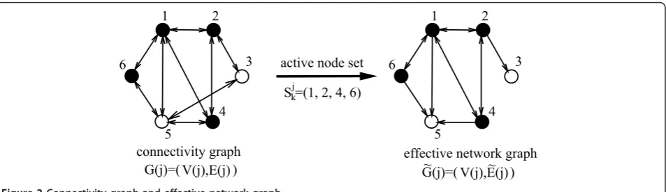
the target in thekth tracking update step as in Figure 1. Figure 2 shows the relation between the connectivity graph G(j) and the effective network graph G˜(j)for a
graph of 6 nodes with active node set Sjk= (1, 2, 4, 6), where solid circles denote active nodes.
Let ISjk denote anN ×N matrix generated from the
active node setSjkas follows:
[ISj k]nn
=
1 ifn=nand n∈Sjk
0 else .
Note that,ISjkis a diagonal matrix with n’th diagonal
element equal to zero forn∈(Sjk)c, where (·)c
denotes the set complement. By combining the connectivity graph G(j) with the active node set Sjk, we obtain the
A
effective network graphG˜(j). Thus, the adjacency matrix
of the effective network graph is given by A(j) =A(j)ISjk.
The corresponding degree matrix D(j) can then be obtained fromA(j), and the Laplacian matrix is L(j) = D (j) -A(j) by definition.
As an example, consider the same network model in Figure 2. The matrix ISjk = diag(1, 1, 0, 1, 0, 1). The
Laplacian matrices of the connectivity graph and effec-tive network graph are as follows:
L(j) =
⎡ ⎢ ⎢ ⎢ ⎢ ⎢ ⎢ ⎣
4−1 0−1−1−1
−1 3−1−1 0 0 0−1 2 0−1 0
−1−1 0 3−1 0
−1 0−1−1 4−1
−1 0 0 0−1 2
⎤ ⎥ ⎥ ⎥ ⎥ ⎥ ⎥ ⎦
and L(j) =
⎡ ⎢ ⎢ ⎢ ⎢ ⎢ ⎢ ⎣
3−1 0−1 0−1
−1 2 0−1 0 0 0−1 1 0 0 0
−1−1 0 2 0 0
−1 0 0−1 3−1
−1 0 0 0 0 1
⎤ ⎥ ⎥ ⎥ ⎥ ⎥ ⎥ ⎦
.
C Distributed tracking with consensus algorithm
In this section, we propose a distributed tracking and consensus algorithm for the above distributed tracking problem over a time-varying graph with incomplete data and noisy communication links. This algorithm is based on the architecture that was first proposed in [29] in the special context of consensus tracking in a satellite sen-sor network for situational awareness.
Figure 3 shows the timing diagram of tracking and consensus updates process in the proposed distributed tracking with consensus algorithm. As in Figure 3, at tracking time stepk, node n is assumed to have com-pleted its consensus iterations corresponding to timek -1. If the output of this consensus update following the (k - 1)th tracking update step is x¯n(k−1,J)with the
associated covariance matrix P¯n(k−1,J), then node n
sets x¯n(k−1|k−1) =x¯n(k−1,J) and
¯
Pn(k−1|k−1) =P¯n(k−1,J). Next, at the kth tracking
update step, each node nwheren∈Sjk, passes its obser-vationyn(k) through its local Kalman filter as follows [1]:
ˆ
xn(k|k−1) =Fx¯n(k−1|k−1), ˆ
Pn(k|k−1) =FP¯n(k−1|k−1)FT+Q,
Kn(k) =Pˆn(k|k−1)HTn
HnPˆn(k|k−1)HTn+Rn −1
,
ˆ
xn(k|k) =xˆn(k|k−1) +Kn(k)
yn(k)−Hnxˆn(k|k−1)
,
ˆ
Pn(k|k) =
I−Kn(k)Hn ˆ
Pn(k|k−1),
(4)
where x¯n(k−1|k−1) =x¯n(k−1,J) with
¯
xn(0,J) =x¯(0) and P¯n(k−1|k−1) =P¯n(k−1,J) with
¯
Pn(0,J) =P0. LetX¯(k−1,j) =x¯1(k−1,j)T,x¯2(k−1,j)T,. . .,x¯N(k−1,j)T
T
.
1 2
3
4 5
6
effective network graph connectivity graph
S =(1, 2, 4, 6) active node set
G(j)=( )~ V(j),E(j)~ G(j)=( )V(j),E(j)
1 2
3
4 5
6
kj
Figure 2Connectivity graph and effective network graph.
B
DenoteP¯(k−1,j)as the covariance matrix correspond-ing toX¯(k−1,j). TheP¯n(k−1,J)in (4) can be obtained
by extracting the nth M ×M main diagonal block of
¯
P(k−1,J).
Node nuses its filtered estimate xˆn(k|k)obtained by
the above tracking update step as the initial estimate for consensus update exchanges by setting x¯n(k, 0) =xˆn(k|k)
with initial covariance matrix
¯
P(k, 0) =Pˆ1(k|k)⊕ ˆP2(k|k)⊕ · · · ⊕ ˆPN(k|k),a where ⊕
denotes the direct sum. On the other hand, for nodes
n∈(Sjk)c, we may arbitrarily set xˆ
n(k|k) =0 and
ˆ
Pn(k|k) =∈IMfor some> 0.
During the (j + 1)th consensus update, each node n
forms a linear estimate of the following form as its con-sensus estimate:
¯
xn(k,j+ 1) =x¯n(k,j) +γn(j) N
l=1
An,l(j)
¯
zn,l(k,j)− ¯zn,n(k,j)
, (5)
where gn(j) is the nth node’s weight coefficient at iterationjand 0≤j<J. We set gn(j) =g(j) forn∈Sjkand
γn(j) = N 1
l=1An,l(j) for n∈S
j
k and
N
l=1An,l(j)= 0. For
node n that does not have local tracking estimate, we assume that it will generate its estimate by averaging the tracking estimates from its neighbors.b
By defining X¯(k,j) = [x1¯ (k,j)T,x2¯ (k,j)T,. . .,x¯N(k,j)T]T,
the consensus update dynamics can be written in vector form as follows:
¯
X(k,j+ 1) =X¯(k,j)−((j)L(j))⊗IM
¯
X(k,j)−((j)⊗IM)¯(j), (6)
where
(j) = diagγ1(j),. . .,γN(j)
,¯(j) =
φ1(j)T· · ·φN(j)T
T
and φn(j) =−l∈n(j)φn,l(j). Note that, from (3),
E[ (j)] =0andsupjE[ ¯(j)2] =η≤N(N−1)u<∞. Let us define ¯e(k,j)to be the error vector at the jth consensus iteration after the kth tracking update:
¯
e(k,j)X¯(k,j)−(1⊗IM)x(k). From (6), it follows that
¯
e(k,j+ 1) = (A(j)⊗IM)e¯(k,j)−
(j)⊗IM
¯ (j) +(A(j)⊗IM)−I
(1⊗IM)x(k),
(7)
where A(j) = IN-Γ(j)L(j). Note that, this coefficient matrix A(j) is slightly different from the one proposed in [29]. In [29],A(j) =˜I(j)−γ(j)L˜(j), where˜I(j)and L˜(j) are the modified identity and Laplacian matrices. The required modification, however, does not lend itself to a convenient relation between the original matrices and the modified ones that can be used in mathematical derivations.
Note that, if the filtered estimate xˆn(k|k)at the end of
the measurement update stage is an unbiased estimate,
then x¯n(k, 0)is also unbiased for alln∈Sjk. From (5),
since x¯n(k,j+ 1) =N1 l=1An,l(j)
N
l=1An,l(j)(x¯l(k,j) +φn,l(j))
for n∈(Sjk)c, then x¯
n(k,j+ 1) is also unbiased for
n∈(Sjk)cifx¯
l(k,j)is unbiased forl∈Sjk. From (7), it can
be shown that the unbiasedness in consensus estimate
¯
X(k,j)can be maintained if matrixA(j) satisfies the con-dition(A(j)⊗IM)−I
(1⊗IM) =0, which is equivalent
to requiring(A(j)−IN)1
⊗IM=0. It follows that the
unbiasedness in consensus estimateX¯(k,j)requires 0 to be an eigenvalue of the Laplacian matrix L(j) with the associated eigenvector 1.cDefine the covariance matrix corresponding to X¯(k,j) as P¯(k,j) =E[e¯(k,j)e¯(k,j)T]. From (7) and unbiasedness condition, it can be easily seen that
¯
P(k,j+ 1) =A(j)⊗IM
¯
P(k,j)(A(j)⊗IM)T
+E
((j)⊗IM)¯(j)¯(j)T((j)⊗IM)
. (8)
As shown in Figure 3, after J consensus iterations, each nodenwill feed x¯n(k,J) back to their local Kalman
filters by setting x¯n(k|k) =x¯n(k,J)and P¯n(k|k) =P¯n(k,J)
before starting next tracking update at timek+1. Recall that hereP¯n(k,J)is thenthM×M main diagonal block
ofP¯(k,J). Algorithm 1 shows a summary of the steps in the proposed distributed tracking with consensus algorithm.
3 Performance analysis
A Conditions for achieving consensus
In this section, we analyze the convergence of the pro-posed distributed tracking with consensus algorithm and the convergence rate. Note that, the proofs of lemmas and theorems in this section are different from those in [16] due to vector state and incomplete data, which results in two stages of consensus process: obtaining complete data from incomplete data and reaching con-sensus on complete data. In the scenarios we consider, we assume that the information exchange rate during the consensus update process is much higher
Algorithm 1 Distributed tracking with consensus algorithm
Initialize: x(0),F, Hn, Q, Rn whilenew data existdo
Kalman filtering in tracking process:
ˆ
xn(k|k−1) =Fx¯n(k−1|k−1)
ˆ
Pn(k|k−1) =FP¯n(k−1|k−1)FT+Q
Kn(k) =Pˆn(k|k−1)HnT
HnPˆn(k|k−1)HTn+Rn
−1
ˆ
xn(k|k) =xˆn(k|k−1) +Kn(k)
yn(k)−Hnxˆn(k|k−1)
ˆ
Pn(k|k) =
I−Kn(k)Hn
ˆ
Pn(k|k−1)
¯
xn(k, 0) =xˆn(k|k)
¯
P(k, 0) =Pˆ1(k|k)⊕ ˆP2(k|k)⊕ · · · ⊕ ˆPN(k|k)
j¬0
whilej≤J- 1do
¯
xn(k,j+ 1) =x¯n(k,j) +γn(j)
N
l=1An,l(j)
zn,l(k,j)−zn,n(k,j)
j¬j+ 1
end while ¯
xn(k|k) =x¯n(k,J)
¯
Pn(k|k) =P¯n(k,J)
k¬k+ 1
end while
compared with the data sampling rate for the tracking updates. Hence, we can assume that J≫ 1,d guarantee-ing enough time for information to be exchanged over the network so that consensus can be reached if the weight {g(j)} is chosen properly. As mentioned above, for a fixedk andJ ≫ 1, the consensus update process after the kth tracking update can be considered as a consensus in estimation problem. Thus, to simplify notation, in the following, we omit the tracking time step indexkin X¯(k,j).
We start by defining the consensus subspaceCas
C={X∈RNM|X=1N⊗a,a∈RM}.
If the consensus algorithm (6) converges to the con-sensus subspace C, each node estimate x¯n(j)will
con-verge to the same value x¯n(j) =afor 1≤n≤N,aÎ ℝM
and consensus is reached over the network. It is well known from the stochastic approximation literature [36] that, in order to ensure asymptotic convergence to con-sensus subspace, the weight coefficientg(j) must satisfy thepersistence conditionas follows
γ(j)>0, ∞
j=0
γ(j) =∞, ∞
j=0
γ(j)2<∞. (9)
We recall the following result on distance properties inℝNM:
Lemma 1: Suppose that X Î ℝNM and consider the orthogonal decomposition X=XC+XC⊥. Then, the
Euclidean distanceρ(X,C) =XC⊥.
In the following, we prove that the consensus algo-rithm given in (6) converges almost surely (a.s.). This is achieved in two steps: First, Lemma 3 proves that the state vector sequence{ ¯X(j)}j≥0converges a.s. to the
con-sensus subspaceC. Theorem 1 then completes the proof by showing that the sequence of component-wise averages{ ¯Xavg(j)}j≥0converges a.s. to a finite random
variable Θ, where X¯avg(j) = N1(1T⊗IM)X¯(j). The proof
of Theorem 1 will require a basic result on convergence of Markov processes from [36], which is restated as
Lemma 2 in our context. Before stating the lemma, however, we need to introduce the notation of [36].
Let{ ¯X(j)}j≥0be a Markov process in ℝNM. Define the
generating opaseratorLcorresponding to{ ¯X(j)}j≥0as
LV(j,X) =EV(j+ 1,X(j+ 1))|X(j) =X−V(j,X),
for functionsV(j,X),j≥0,X∈RNM, provided the con-ditional expectation exists. If DLis the domain of L, then we say thatV(j,X)∈DLin a domainC, ifLV(j,X) is finite for all(j,X)∈C.
For G⊂ℝNM, the -neighborhood ofGand its com-plement are defined as,
Uε(G) =
X|inf
Y∈Gρ(X,Y)< ε
, Vε(G) =RNM\Uε(G).(10)
With these notations, we may now state the desired lemma on the convergence of Markov processes:
Lemma 2 (Convergence of Markov Processes): Let
{ ¯X(j)}j≥0be a Markov process with generating operator
L. Let there exist a non-negative functionV(j,X)∈DL
in the domainG⊂ℝNM forj≥0 andX∈RNM. Assume
that
inf
j≥0,X∈Vε(G)V(j,X)>0, ∀ε >0, and V(j,X) = 0, X∈G,
lim X→Gsupj≥0
V(j,X) = 0, and LV(j,X)≤g(j)(1 +V(j,X))−γ(j)ϕ(j,X),
whereϕ(j,X),X∈RNMis a non-negative function such that
inf
j,X∈Vε(G)ϕ(j,X)>0, ∀ε >0;γ(j)>0,
j≥0
γ(j) =∞;
and g(j)>0,
j≥0
g(j) =∞.
Then, the Markov process{ ¯X(j)}j≥0with an arbitrary
initial distribution
converges almost surely (a.s.) toGasj®∞:
P
lim
j→∞ρ(X(j),G) = 0
= 1.
Proof Proof is a vector generalization of that in [16], and is omitted.
Lemma 2 guarantees a.s. convergence of a general Markov process with an arbitrary initial distribution under the assumption of the existence of a Lya-punov function V(j,X). In fact, the state vector sequence
{ ¯X(j)}j≥0 given in (6) is a Markov process, since P[X(j)|X(j−1),. . .,X(0)] =P[X(j)|X(j−1)]. In the next lemma, we prove that the state estimate sequence
{ ¯X(j)}j≥0given in (6) converges a.s. to the consensus
over an undirected effective network graph satisfies the Lyapunov function assumptions of Lemma 2.
Lemma 3 (a.s. convergence of the proposed algorithm to the consensus subspace): Consider the consensus algo-rithm in (6) with initial state X(0)∈RNM. The weight
coefficients satisfy the persistence condition in (9). Assume that the undirected connectivity graph Lapla-cian L(j) is independent ofcommunication noisejn,l(j) for 1≤ n, l≤ N. If L(j) =L+L˜(j)with mean L=E[L(j)] is such that λ2(L)>0and p(l, n) > 0 for {l, n} Î E(j),
then
P
lim
j→∞ρ(X(j),C) = 0
= 1.
ProofSee Appendix A.
Lemma 3 shows that the state estimate sequence
{ ¯X(j)}j≥0given in (6) converges a.s. to the consensus
subspace C. The key to the proof is to show that the directed effective network graph will become an undir-ected graph after all nodes have local estimates and the consensus algorithm over this undirected effective net-work graph satisfies the condition required in Lemma 2. In the following theorem, we state our main result and complete the convergence proof for the proposed dis-tributed tracking with consensus algorithm by showing that the sequence of component-wise averages
{ ¯Xavg(j)}j≥0converges a.s. to a finite random variable Θ,
whereXavg¯ (j) = N1(1T⊗IM)X¯(j).
Theorem 1 (a.s. convergence to a finiterandom vector): Consider the consensus algorithm in (6) with initial state X(0)∈RNM. The weight coefficients satisfy the
persistence condition in (9). Assume that the time-vary-ing connectivity graph Laplacian L(j) is independent of communication noise jn,l(j) for 1 ≤ n, l ≤ N. If
L(j) =L+L˜(j) with mean L=E[L(j)] is such that
λ2(L)>0, and ifp(l, n) > 0 for {l, n}Î E(j), then there
exists an almost sure finite real random vector Θsuch that
P
lim
j→∞X(j) = 1N⊗
= 1.
Proof Since the mean connectivity graph Lis con-nected with non-zero link probability, forjlarge enough, each node will receive information from one another and generate its updated local estimate. For a fixedk, let
Jk= inf{j|(Sjk)c=0,j≥0}. Then, Γ(j) = g(j)IN for j ≥ Jk and (6) becomes
X(j+ 1) =X(j)−γ(j)(L(j)⊗IM)X(j) + (j)
for j≥Jk. (11)
Define the average ofX¯(j)asXavg¯ (j) =N1(1T⊗IM)X¯(j).
Multiply both sides of (11) by N1(1T⊗I
M)and use the
fact that1TL(j) =0N, so that for(Sjk)c=0, we have
Xavg(j+ 1) =Xavg(j)−ε(j) =Xavg(Jk)−
Jk≤l≤j
ε(l),
whereε(j) = γN(j)(1T⊗I
M) (j). Assuming that receiver
noise is zero-mean and time independent, we obtain
E[ε(j)2] = γ
2(j)
N2 E[¯(j) T(1T⊗I
M)T(1T⊗IM) (j)]
= γ
2(j)
N2 E
⎡
⎣
1≤n≤N
(φn(j))Tφn(j) ⎤ ⎦,
where φn(j) =−l∈n(j)φn,l(j) denotes the total
incoming noise from nodelÎ Ωn(j) to nodenand the last step follows from the independence of jl(j) andjn (j). By assuming thatEφl,n(j)φl,n(j)T
=σ2I
M, for 1 ≤l,
n≤N, we obtain
E[ε(j)2]≤ γ
2(j)
N2 MN(N−1)σ
2=γ2(j)M(N−1)
N σ
2.
From independence ofX¯(j)and (j)and the indepen-dence of noise over time, we then have that
E[Xavg(j+ 1)2]≤E[Xavg(Jk)TXavg(Jk)] + j
l≥Kk
γ2(l)M(N−1)
N σ
2≤ ∞.
Denote Xavg(j) = [Xavg,1(j). . .Xavg,M(j)]T. It can be
easily seen that
E[(Xavg,m(j+ 1))2]≤E[(Xavg,m(Jk))2] + j
l≥Jk
γ2(l)(N−1)
N σ
2≤ ∞.
Hence, the sequence{Xavg,m(j)}is anL2 bounded mar-tingale and thus converges a.s. inL2 to a finite random scalar θ. Define Xm(j) = [eTmx1¯ . . ., e
T
mx¯N]T. From the
conclusion of Lemma 3, we have that
P[limj→∞X(j)−1N⊗Xavg(j)= 0] = 1, which
implies that
P[limj→∞Xm(j)−Xavg,m(j)1N= 0] = 1. Then, we
obtain that
P[limj→∞Xm(j) =θ1N] = 1and the theorem follows.
Theorem 2 (convergence rate):Consider the consensus algorithm in (6) with initial state X(0)∈RNM. The
weight coefficients satisfy the persistence condition in (9) andγ(j)≤ λ 2
2(L)+¯ λn(L)¯ . Assume that the time-varying connectivity graph LaplacianL(j) is independent of com-munication noise jn,l(j) for 1≤n, l≤ N. Forj≥ Jk, the effective network graph Laplacian isL(j) = L +L(˜ j)with mean L =E[L(j)]. If the connectivity graph LaplacianL
(j) with meanL=E[L(j)]is such thatλ2(L)>0, and ifp
(l, n) > 0 for {l, n}Î E(j), the convergence rate,e of the proposed consensus algorithm is bounded by
−λ2(L)
1 J−Jk
Jk≤j≤Jγ(j)
.
ProofFor a fixedi, let Jk= inf{j|(Sjk)c=∅,j≥0}. From
the asymptotic unbiasedness of Θ, we have limj→∞E[X(j)] =1N⊗r, where r=Xavg(Jk). For j ≥ Jk, define (j) =INM=−γ(j)(L⊗IM), where L =E[L(j)].
Using the fact that L(j) andX¯(j)are independent, and
E[¯(j)] =0NM, from (6), we have that
E[X(j+ 1)] =(j)E[X(j)] =
j
l=Jk
(l)E[X(Jk)], ∀j≥Jk. (12)
From the persistence condition
γ(j)>0,j≥0γ(j) =∞andj≥0γ2(j)≤ ∞[16], it
fol-lows thatg(j)®0. From the mixed-product property of Kro-necker product (A⊗ B)(C ⊗D) =AB ⊗CD and (INM−γ(j)L)1N=1N[32], we have
1N⊗r=(j)(1N⊗r). (13)
From (12) and (13), it can be shown that
E[X(j)]−1N⊗r ≤
Jk≤l≤j−1
¯
ρ(1−γ(l)L)E[X(Jk)]−1N⊗r
=
Jk≤l≤j−1
(1−γ(l)λ2(L))E[X(Jk)]−1N⊗r,
where last step follows from Lemma 8 of [15] andρ¯(·) denotes the spectral radius of a matrix. From the assumption on weight coefficient g(j), we have 0≤γ(l)λ2(L)¯ ≤1. Since 1 - a ≤e-a for 0 ≤ a ≤ 1, we
then have that
E[X(j)]−1N⊗r≤
e−λ2(L)¯Jk≤l≤j−1γ(l)
E[X(Jk)]−1N⊗r. (14)
Therefore, as j® J, the convergence rate is bounded by −λ2(L)¯
1 J−Jk
Jk≤l≤Jγ(l)
, which depends on the
algebraic connectivityλ2(L)and the weightsg(j), forJk≤
j≤J.
Theorem 2 shows that the convergence rate of the proposed algorithm depends on the topology through the algebraic connectivityλ2(L)of the effective network
graphG˜(j)and through weightsg(j), forj≥Jk. Since for ¯
L =E[L(j)] =E[L(j)] and L(j) = L(j), we have
¯
L =E[L(j)] =E[L(j)]. In (14), λ2(L)is the algebraic
con-nectivity of the mean Laplacian corresponding to the time-varying network graphs. For a static network, this reduces to the algebraic connectivity of the static Lapla-cian L.
Since the consensus algorithm in (6) is iterative, whose energy consumption is proportional to the time neces-sary to achieve consensus and inversely proportional to transmit power. From [38,39], for energy-constrained sensor networks, there exists a tradeoff between conver-gence time that depends on network connectivity and the transmit power of each node necessary to establish the links with the desired reliability. Therefore, we can minimize the energy consumption for consensus process by optimizing transmit power, network topology, and weightsg(j).
B Steady-state analysis for noiseless graphs
In this section, we analyze the steady-state performance of the proposed distributed tracking with consensus algorithm. When the filter reaches steady state, the error covariance matrix is time invariant and the corre-sponding filter gain is constant. Therefore, finding the steady state of the proposed algorithm will help under-standing its asymptotic behavior, analyzing error covar-iance, and filter design. From (8), it can be seen that the propagation of communication noise implies the non-existence of an upper bound to the covariance matrix. Therefore, the covariance matrix in the Kalman filter may not also converge and the filter may not reach steady state. However, time-varying graph assumption does not affect the existence of steady state. Since forJ
® ∞, consensus is reached over the network and the outputs of the consensus update Xn(k,J)and P(k,J)
depend only on the inputsXn(k, 0)andP(k, 0)for
com-plete data case with noiseless time-varying graphs (for incomplete data case with noiseless time-varying graphs, this property still holds for some special types of graphs). Hence, the combined system of distributed tracking with consensus can be transformed into a Kal-man filter with time-invariant parameters. Therefore, steady state can still be reached [1]. In the following, assuming noiseless time-varying graphs, we start with steady-state analysis for the case with complete data, and then, we extend the results to the case with incom-plete data.
1) Complete data with noiseless time-varying graphs
Here, we assume complete data, a scalar target state xÎ ℝ1
(for simplicity) and noiseless time-varying graphs, where the connectivity graph Laplacian L(i) with mean
ˆ
Pn(k+ 1|k)cannot be easily obtained when the target
statexÎ ℝMforM > 1, the following derivation would not apply to vector state.
From the result of Theorem 1 for scalar target state, itcan be shown thatlimJ→∞X(k,J) =Xavg(k, 0)1N, where Xavg(k,j) = N11TX(k,J). From the definition ofX(k,j)and
¯
xn(k, 0) =xˆn(k|k), we have for 1≤n≤N
lim
J→∞x¯n(k,J) = 1 N N n=1 ˆ
xn(k|k). (15)
With the assumptions above, the covariance matrix (8) in the (j+ 1)th consensus iteration after thekth tracking update simplifies to P(k,j+ 1) =A(j)P(k,j)A(j)T For
complete data case, L(j) =L(j). Since 1T L(j) = 0, from (7), we have1TA(j) =1. Then, we can obtain that
1TP(k,j+ 1)1=1TP(k,j)1. (16)
By applying the result of Theorem 1, we have limJ→∞P(k,J) = (Xavg(k, 0)−x(k))211T. Since all the
elements inlimJ→∞P(k,J)are equal, from (16), it
fol-lows that
lim
J→∞P(k,J) =
1TP(k, 0)1 N2 11
T=
N
n=1Pˆn(k|k)
N2 11 T. (17)
SinceP¯n(k,J)is thenthM×Mmain diagonal block of
¯
P(k,J), we have the covariance matrix for noden(1 ≤n ≤N) as below:
lim
J→∞Pn(k,J) =
N
n=1Pˆn(k|k)
N2 . (18)
From (15) and (18), we have x¯n(k,J) =¯xl(k,J) and
¯
Pn(k,J) =P¯l(k,J)for J®∞and 1≤n, l≤N. Then, each
node n sets x¯n(k|k) =x¯n(k,J) and Pn(k|k) =Pn(k,J).
From (4), we have ˆxn(k+ 1|k) =xˆl(k+ 1|k) and
ˆ
Pn(k+ 1|k) =Pˆl(k+ 1|k)for 1≤ n, l ≤ N and it follows
that for 1≤n≤N
ˆ
xn(k+ 1|k) =F
1 N N q=1 ˆ
xq(k|k−1)−F
1 N N q=1
Kq(k)(yq(k)−Hqxˆq(k|k−1))
,
ˆ
Pl(k+ 1|k) =Q+
1
N2 N
q=1
F(I−Kq(k)Hq)Pˆq(k|k−1)FT.
(19)
Let xˆn(k+ 1|k) =xˆ(k+ 1|k) and
ˆ
Pn(k+ 1|k) =Pˆ(k+ 1|k). Then, the combined system of
distributed tracking with consensus can be transformed into a single Kalman filter as follows:
ˆ
x(k+ 1|k) =Fxˆ(k|k−1) +F
N
N
n=1
Kn(k)(yn(k)−Hnxˆn(k|k−1))
,
Kn(k) =Pˆ(k|k−1)HTn
HnPˆ(k|k−1)HTn+Rn
−1
,
ˆ
P(k+ 1|k) =Q+ 1
N2 N
n=1
FPˆ(k|k−1)FT−FK n(k)
HnPˆ(k|k−1)HTn+Rn
×Kn(k)TFT
.
(20)
Theorem 3 Consider the system dynamics in (1) and (2) and the Kalman filter in (20). Assume that the con-nectivity graph Laplacian L(j) with mean L=E[L(j)]is such that λ2(L)>0, andp(l, n) > 0 for {l, n}Î E(j). If
the pair (F, Hn) is observable for 1 ≤n ≤ N, then the prediction covariance matrixPˆ(k|k−1)converges to a constant matrix
lim
k→∞Pˆ(k|k−1) =P,
whereP is the unique definite solution of the discrete algebraic Riccati equation (DARE)
P=Q+ 1
N2
N
n=1
FPFT−FPHTn(HnPHTn+Rn)−
1
HnPFT
. (21)
Proof See Proof of Theorem 4. By settingm=Nand bn(k) = 1 for 1≤n≤N, the Kalman filter in (24) can be reduced to the one in (20). Theorem 3 can be consid-ered as a special case of Theorem 4. Thus, it can be proved in a similar manner.
As a consequence of Theorem 3, the local Kalman fil-ter gain converges to
lim
k→∞Kn(k) =PH
T
n[HnPHTn+Rn]−1.
From (21), it can be seen that limN®∞P =Q, i.e., as
the size of the sensor networkNincreases, the steady-state covariance P, which in this case is a scalar, will decrease. This implies that if the network size is large enough, asymptotically the tracking is noiseless and fol-lows the target exactly. It is obvious that this result still holds for distributed local Kalman filtering with centra-lized fusion. However, the distributed tracking with con-sensus results in the same performance even if the graph is time-varying and it also improves the robust-ness and scalability due to consensus exchanges. For the assumed scalar case, for example, ifHn=HandRn=R for 1 ≤ n ≤ N, then we have K= HHP2P+R and
P= −B+
√
B2+4H2QR
2H2 , where B=
1− FN2R−H2Q. This
implies that for the same sensing model, each node will have the same Kalman gainKand prediction covariance
Pin the steady state.
2) Incomplete data with noiseless time-varying graphs
Next, we assume incomplete data, a scalar target statex
Î ℝ1
and noiseless time-varying graphs, where the con-nectivity graph Laplacian L(j) with mean L=E[L(j)]is such that λ2(L)>0, and p(l, n) > 0 for {l, n} Î E(j).
Furthermore, we assume that only mnodes can observe the target and without loss of any generality the index of those mnodes are ordered as 1, 2,..., m, wheremis constant and 1 ≤ m≤ N. This implies that the active node set S0
further assumptions on the connectivity graph for con-sensus, since the graph is connected on average and the information can still propagate over the network even if only a fixed number of nodes have observation.
With the assumption of incomplete data and noiseless time-varying graphs, 1TL(j) = 0 forJk≤j<J. Then, (17) becomes
lim J→∞P(k,J) =
1TP¯(k,J
k)1
N2 11 T=1
TAJk−1
0
P(k, 0)AJk−1
0 T
1
N2 11 T
= m
n=1Pˆn(k|k)βn2(k)
N2 11 T,
(22)
where AJk−1
0
=A(Jk−1)· · ·A(0) and
βn(k) =Nl=1AJk−1 0
lnis thenth column sum of
AJk−1 0
that depends on time k. The last step of (22) follows from that Pˆn(k|k) =εfor m <n ≤ N and some > 0.
Then, as in previous subsection, we have for 1≤n≤N
lim
J→∞P¯n(k,J) =
m
n=1Pˆn(k|k)βn2(k)
N2 , and
lim
J→∞¯xn(k,J) = 1 N m n=1 ˆ
xn(k|k)βn(k).
(23)
From (23), for J ® ∞, we have x¯n(k,J) =¯xl(k,J)and
Pn(k,J) =Pl(k,J) for 1 ≤ n, l ≤ N. By setting
¯
xn(k|k) =x¯n(k,J)andPn(k|k) =Pn(k,J), from (4), we can
obtain recursive update equations for Pˆn(k+ 1|k)and
ˆ
xn(k+ 1|k). Furthermore, we also have
ˆ
xn(k+ 1|k) =xˆl(k+ 1|k)and Pˆn(k+ 1|k) =Pˆl(k+ 1|k)for
1 ≤ n, l ≤ N. Let xˆn(k+ 1|k) =xˆ(k+ 1|k) and
ˆ
Pn(k+ 1|k) =Pˆ(k+ 1|k). Then, the combined system of
distributed tracking with consensus can then be trans-formed into a single Kalman filter for node n(1 ≤ n ≤ m) as below:
ˆ x(k+ 1|k) =F
N m
n=1 ˆ
x(k|k−1)βn(k) + F N m n=1
Kn(k)(yn(k)−Hnˆx(k|k−1))βn(k)
,
Kn(k) =Pˆ(k|k−1)HTn
HnPˆ(k|k−1)HnT+Rn
−1
,
ˆ
P(k+ 1|k) =Q+ 1
N2 m
n=1
FPˆ(k|k−1)FT−FK n(k)
HnPˆ(k|k−1)HTn+Rn
×Kn(k)TFT
β2 n(k),
(24)
where (20) is a special case of (24) withm=Nand bn (k) = 1 for 1≤n≤N.
Theorem 4 Consider the system dynamics in (1) and (2) and the Kalman filter in (24). Assume thatmnodes can observe the target and the index of those mnodes are fixed and ordered as 1,...,m. The connectivity graph Laplacian L(j) with mean L=E[L(j)] is such that
λ2(L)>0, andp(l, n) > 0 for {l, n}Î E(j). The
connec-tivity graph has switching topologies and is periodic such thatbn(k) = bnis time invariant. If the pair (F, Hn)
is observable for 1 ≤n≤ m, then the prediction covar-iance matrixPˆ(k|k−1)converges to a constant matrix
lim
k→∞Pˆ(k|k−1) =P,
whereP is the unique definite solution of the discrete algebraic Riccati equation (DARE)
P=Q+ 1
N2
m
n=1
FPFT−FPHTn(HnPHTn+Rn)−
1
HnPFT
β2
n. (25)
ProofSee Appendix B.
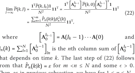
Theorem 4 asserts that if the connectivity graph topol-ogy is switching and periodic, the proposed algorithm can still reach steady-state and the steady-state covar-iance matrix can be obtained by solving (25). The condi-tions of graph topology assumed in Theorem 4 are strong. However, it may still be applicable in certain situations such as satellite surveillance network in [29], since the existence of a communication link depends on distance between nodes and the trajectories of satellites are pre-determined and periodic, whenever ratios of the orbit periods are rational. As an example, consider the network model in Figure 4. The connectivity graph in Figure 4 is switching and periodic with period equal to 4, and it can be seen that the graph is connected on average. Let N= 6,m= 4,S0
k ={1, 2, 3, 4}andγ(j) = 1 j+1
for 0 ≤ j <J. After iterationJk = 1, all nodes will have updated local estimates to be shared. In this case,
AJk−1 0
becomes
AJk−1
0 = ⎡ ⎢ ⎢ ⎢ ⎢ ⎢ ⎢ ⎣
−1 1 0 1 0 0 1−2 1 1 0 0 0 1 0 0 0 0 1 1 0−1 0 0
1
3 0
1 3
1 30 0
1 0 0 0 0 0 ⎤ ⎥ ⎥ ⎥ ⎥ ⎥ ⎥ ⎦ .
It can be seen that
AJk−1 0
is time-variance ofm and the periodic graph topology. Thus, bn(k) = bn is also time invariant and N1mn=1βn= 1, which follows from the condition for unbiasedness in the consensus esti-mate X(k,j). As we will see shortly, from the simulation results in Section IV, the filter indeed reaches steady state in this case, and then, the error covariance matrix becomes time invariant and the corresponding filter gain is constant.
4 Numerical examples
performance of the centralized Kalman filter is well-understood [40] and provides a benchmark performance for distributed local Kalman filtering with centralized fusion. In distributed local Kalman filtering with centra-lized fusion, all nodes send their filtered estimates to a fusion center. The fusion center then generates a fused estimatexˆfusion(k) = |S10
k|
n∈S0
kxˆn(k|k).
In the first simulation, we compare the performance of the proposed algorithm with the distributed local Kalman filtering with centralized fusion and the centralized Kal-man filter over a random graph with noisy communica-tion links and incomplete data. We consider a random connectivity graphG(N, p) withN= 20 and the probabil-ity that each link existsp= 0.5. The other parameters of the simulation setup are:F= 1,Q= 1,x(0) = 0,P0= 0,Rn = 0.25,Hn= 1,σl2,n=σ2= 0.1,S0k ={n|1≤n≤10,n∈Z}
andJ= 30.
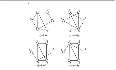
Figure 5a shows the node estimates of the three algo-rithms in a time-varying graph with noisy communica-tion links. As we can see, the node estimates of the three algorithms follow the target’s trajectory. In Figure 5a, the curve with cross marker denotes the first node’s estimate by using distributed tracking with consensus algorithm, the dashed curve denotes the distributed local Kalman filtering with centralized fusion, and the curve with circle marker denotes the centralized Kalman
filter and the solid curve denotes the target’s trajectory. Figure 5b compares the resulting mean squared error (MSE) of the three algorithms, where the MSE of the distributed tracking with consensus is defined to be the
average MSE over all nodes
1 N
N
n=1
(x¯n(k,J)−x(k))T(x¯n(k,J)−x(k))
. In Figure 5b, it can be seen that the MSE of the proposed distrib-uted tracking with consensus algorithm is close to that of the distributed local Kalman filtering with centralized fusion. As expected, both of them are higher than the MSE of the centralized Kalman filter, which acts as a benchmark. The results in Figure 5 show that the per-formance of the proposed distributed tracking with con-sensus algorithm is close to that of the distributed local Kalman filtering with centralized fusion in a time-vary-ing random graph with noisy communication and incomplete data. Additional communication bandwidth, which depends on graph topology Gand number of iterationsJ, is required for the proposed algorithm due to information exchange among nodes. However, it resolves the bandwidth constraints problem of fusion center for centralized fusion case and has a high level of fault tolerance and reliability. Also, because of its advan-tages of fully distributed implementation, robustness, and scalability, it may be preferable in practical applications.
B
In the second simulation, we consider the two-dimen-sional tracking problem treated in [22]. The connectivity graph is again assumed to be a random graph G(N, p) withN= 50 and the probability that each link existsp= 0.5. The probability of each node having an observation at a given time instant isps= 0.9. The other parameters of the simulation setup are as follows:
F=I2+εF0+ε
2
2F 2 0+ε
3
6F 3 0,F0=
0−2 2 0
,ε= 0.015,Q= (εc2
w)2I2,cw= 5,x(0) = [15,−10]T,Hn= [1, 0]
for nis odd and Hn= [0, 1] for nis even,Rn=c2v
√ nfor
n = 1, . . ., N with cv = 30,σl2,n=σ2= 1,J= 10. Note
that, the target is moving on noisy circular trajectories. The target is not fully observable by an individual node, but is collectively observable by all nodes.
0 10 20 30 40 50
í12
í10
í8
í6
í4
í2 0 2 4
tracking time step (k)
node estimates
the proposed algorithm
distriubted Kalman filtering with centralized fusion centralized Kalman filter
target
0 10 20 30 40 50
0 0.05 0.1 0.15 0.2 0.25 0.3 0.35 0.4 0.45 0.5
tracking time step (k)
MSE
the proposed algorithm
distributed Kalman filtering with centralized fusion centralized Kalman filter
A
B
Figure 6a shows the node estimates (trajectory) of the two algorithms over a time-varying graph with incom-plete data. In Figure 6a, the curves with markers denote all the node estimates by using distributed tracking with consensus algorithm, while the dashed curve denotes the distributed local Kalman filtering with centralized fusion and the solid curve denotes the target’s trajectory. As we can see, both algorithms overcome the impact of partial observations at each node resulting in improved overall observation quality and the node estimates by using distributed tracking with consensus algorithm are noisy due to the communication noise. Note that the estimates are close to the trajectory of the target but with a small gap. That is because the observation noise covariance is rather large at each node. Figure 6b com-pares the resulting MSE of these algorithms. It can be seen that the mean squared error of the proposed algo-rithm is slightly higher than that of the distributed Kal-man filtering with centralized fusion.
Next, we study the steady-state behavior in the case of time-varying graphs with complete data and noiseless communication. We consider a random connectivity graph G(N, p) with N= 6 and the probability that each link existsp= 0.5. The other parameters of the
simula-tion setup are as follows:
F= 1,Q= 1,x(0) = 0P0= 0.5,Rn= 0.25,σl2,n=σ2= 0,J= 30,Hn= 1.
Figure 7a shows the node consensus estimates x¯n(k,J)
over a random graph with noiseless communication links and complete data. It can be seen that all node estimates x¯n(k,J) converge to the same value and follow
the target state, as asserted by Theorem 1. Figure 7b and 7c shows the node estimates x¯n(k,J) in the
consen-sus update after the twenty-first tracking update and the variance of all the node estimates, respectively. Here, the variance of all the node estimates is defined as (k,j) =E
(x¯n(k,j)−μ(k,j))T(x¯n(k,j)−μ(k,j))
, where
μ(k,j) = 1 N
N
n=1x¯n(k,j). From Figure 7b, it can be seen
that the node estimates converge to the average which is also confirmed in Figure 7c, where the variance var(k, j) decreases as consensus iteration number increases and becomes static (around 10-17) after consensus is reached. Figure 8 shows the node estimate variance
ˆ
Pn(k|k−1)and Kalman gainKn(k) of the filter in (20). It can be seen that as the Kalman filter reaches steady state, both the node estimate variance and the Kalman gain converge, as asserted by Theorem 3.
Next, we study the steady-state behavior on a graph with switching topologies and incomplete data and noiseless communication. The assumed parameters in the first simulation setup are as follows: F= 1,Q= 1,x(0) = 0,P0= 0.5,Rn= 0.25,σl2,n=σ2= 0,N= 6,J= 40,S0k=
{1, 3, 4, 6},Hn= 0.5
for n= 1, 3 andHn = 1 for n= 4, 6. The connectivity graph Laplacian is
L(j) = ⎧ ⎪ ⎪ ⎨ ⎪ ⎪ ⎩
L1j= 4m L2j= 4m+ 1 L3j= 4m+ 2 L4j= 4m+ 3
for m= 0, 1, 2,. . .,
which is shown in Figure 4. As we can see, the graph is connected on average andp(l, n) > 0 for {l, n}Î E(j), satisfying the conditions on the connectivity graph Laplacian required in Theorem 1.
Figure 9 shows the prediction covariance matrix
ˆ
Pn(k|k−1)and Kalman gainKn(k) of the filter in (20), respectively. It can be seen that as the Kalman filter reaches the steady state, both the prediction covariance matrix and the Kalman gain converge, as asserted by Theorem 4. Note that the limit of the Kalman gain is different for different nodes in Figure 9 because the observation matrixHnis different for different nodes.
5 Conclusions
In this paper, we considered the problem of distributed tracking with consensus on a time-varying graph with incomplete data and noisy communication links. We developed a framework consisting of tracking and con-sensus updates to handle the issues of time-varying net-work topology and incomplete data. We discussed the conditions for achieving consensus, quantified the con-vergence rate and analyzed the steady-state performance when applicable. Our simulation results showed that the proposed distributed tracking with consensus algorithm improves the estimation quality at each node and its performance is close to that of the distributed local Kal-man filtering with centralized fusion. The proposed algorithm shows advantages of fully distributed imple-mentation, robustness and scalability, which is preferable in practical application.
Appendix A Proof of Lemma 3
Proof Since λ2(L)>0and p(l, n) > 0 for {l, n}Î E(j),
the undirected time-varying connectivity graph G(j) is connected on average with non-zero link probability. For jlarge enough, each node will receive the informa-tion from one another and generate its updated local estimates. For a fixed k, let Jk= inf{j|(Sjk)c=∅,j≥0}.
Then, we have the effective network graph is the same as connectivity graphG˜(j) =G(j), L(j) =L(j)andΓ(j) =g (j)INforj≥Jk.
V(j,X) =XT(L⊗IM)X. Since we assume the graph is
undirected and connected on average,Lis positive semi-definite. Then, the potential function V(j,X)is non-negative. Since XεCis an eigenvector of L⊗IMwith
zero eigenvalue,V(j,X)≡0,X∈C, limX→Csupj≥0V(j,X) = 0.
From Courant-Fisher Theorem [31,41], for Z Î ℝN M andZ⊥C, we have
ZT(L⊗IM)Z≥λ2(L⊗IM)ZTZ. (26)
A
0 50 100 150 200 250
0 5 10 15 20 25 30 35
tracking time step (k)
MSE
the proposed algorithm
distributed Kalman filtering with centralized fusion
B