Passive hypervelocity boundary layer control using an acoustically absortive surface

(1)

Passive Hypervelocity Boundary Layer Control Using an

Ultrasonically Absorptive Surface

Thesis by Adam Rasheed

In Partial Fulfillment of the Requirements for the Degree of

Doctor of Philosophy

1 8 9 1

C A L

IF

O

RN IA

IN

STI T U

T E_{O F}

T

E

C

H N

O

L

O

G Y

California Institute of Technology Pasadena, California

2001

(2)

c

(3)

Acknowledgments

It is with my deepest gratitude that I thank my advisor, Professor Hans G. Hornung, for not only guiding my quest for scientific knowledge, but also for encouraging me to explore and appreciate life in itself. I would also like to thank our collaborators, Alexander Fedorov and Norm Malmuth, whose assistance was invaluable throughout this project. Special recognition is due to Bahram Valiferdowsi who, for the past four years, has not only been a valuable friend, but also kindly and patiently showed me how to design, machine, build and repair anything and everything.

On a more personal level, it goes without saying that I must acknowledge the role of my family in my development and education. I am eternally grateful to my sister who, among other things, showed me how to take my first derivative and my cousin who first introduced me to the world of engineering. As for my parents, uncle and aunt, their contribution is beyond words. I would also like to thank all my friends here at Caltech who entertained or annoyed me when I wasn’t working and have made my stay here enjoyable.

Lastly, I would like to acknowledge the late Professor Bradford Sturtevant who originally provided me with the opportunity to study at Caltech and to whom I am forever indebted. His tenacity and excitement for science will be sorely missed.

(4)

Abstract

(5)

List of Figures

1.1 Laminar versus turbulent viscous drag on a hypersonic transport . . . 2

1.2 Total heat and heat transfer rate for a reentry vehicle . . . 3

1.3 Heat transfer rates for a trans-atmospheric hypersonic vehicle . . . 4

1.4 Schematic diagram of the Mack mode in the boundary layer . . . 8

1.5 Growth rate of first and second mode as a function of Mach number . . . . 9

1.6 Illustration of boundary layer transition process . . . 12

1.7 Amplification rates for typical T5 shots computed using thermochemical non-equilibrium linear stability analysis . . . 15

2.1 Amplification rates from inviscid linear stability analysis with wall reflection coefficient as a parameter . . . 22

2.2 Amplification rates from viscous linear stability analysis with wall reflection coefficient as a parameter . . . 24

2.3 Schematic diagram of the porous microstructure . . . 25

2.4 Amplification rates with hole radius as a parameter . . . 29

2.5 Growth rates as functions of the porosity and depth of the holes . . . 29

2.6 Diagram of the acoustic model for an individual hole . . . 31

2.7 Circuit diagram used to represent an electric transmission line . . . 35

2.8 Diagram of the motion of the gas in narrow and wide holes . . . 47

2.9 Calculated radial variation of the disturbance quantities in a hole . . . 49

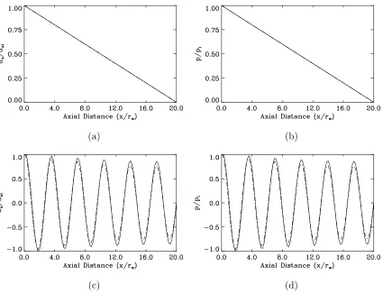
2.10 Axial variation of normalized particle velocity and pressure perturbation within a hole . . . 50

2.11 Schematic drawing showing porous surface to scale . . . 55

2.12 Calculated radial variation of the disturbance quantities for the expected experimental conditions . . . 56

2.13 Axial variation of normalized particle velocity and pressure perturbation within a hole at the expected experimental conditions . . . 57

(10)

3.2 Diagram of the test model . . . 64

3.3 Micrograph of the weld and the perforated sheet . . . 65

3.4 Diagram of the measured cross-section of the cone . . . 67

3.5 Micrograph of new and blunted cone tips . . . 68

3.6 Diagram of the thermocouple layout on the test model . . . 70

3.7 Photograph of the 90◦ flat plate test piece . . . 72

3.8 Photograph of the 5◦ cylinder test piece . . . 73

3.9 Typical time-resolved temperature and heat transfer data trace . . . 81

3.10 Typical non-dimensional spatial heat flux distribution . . . 82

4.1 Typical non-dimensional spatial heat flux distribution used to determine transition location . . . 87

4.2 Typical plot of cumulative sum of recursive residuals . . . 89

4.3 Transition Reynolds number versus stagnation enthalpy . . . 90

4.4 Reference transition Reynolds number versus stagnation enthalpy . . . 91

4.5 Stanton number versus Reynolds number for shot 1960 . . . 94

4.8 Summary plot of the nitrogen transition data . . . 98

4.9 Summary plot of the carbon dioxide transition data . . . 99

4.10 Effect of surface roughness on the transition data . . . 102

4.11 Resonantly enhanced shadowgraph for shot 2008 . . . 105

C.1 Micrograph of the polyester perforated sheet . . . 137

C.2 Micrograph of the stainless steel perforated sheet . . . 138

C.3 Micrograph of the final porous surface . . . 138

C.4 Micrograph of the weld joining the perforated and solid sheets . . . 140

C.5 Micrograph of thermocouple mounted in a test piece . . . 142

C.6 Micrograph of Feltmetal product . . . 143

(11)

List of Tables

2.1 Summary of the electrical analogy . . . 40

3.1 Measured steps at cone junctions . . . 65

A.1 Summary of the freestream conditions for the N₂ shots . . . 124

A.2 Summary of the edge and reference conditions for the N₂ shots . . . 125

A.3 Summary of the transition data for the N₂ shots . . . 126

A.4 Freestream molecular weight and species concentrations for the N₂ shots as computed by NENZF . . . 127

A.5 Summary of the freestream conditions for the CO₂ shots . . . 128

A.6 Summary of the edge and reference conditions for the CO₂ shots . . . 129

A.7 Summary of the transition data for the CO₂ shots . . . 130

A.8 Freestream molecular weight and species concentrations for the CO₂shots as computed by NENZF . . . 131

C.1 Calculated thermal interference strains . . . 141

(12)

Chapter 1

Introduction

1.1

Motivation

The introduction of the concept of the boundary layer by Prandtl at the turn of the century was a watershed moment in the history of fluid mechanics. For the first time, it brought theoretical considerations, which at the time were based almost entirely on Euler’s inviscid relations, into agreement with experiments. It was quickly realized that the state of the boundary layer had an enormous impact on the skin friction (viscous) drag of a body. Furthermore, the boundary layer readily transitioned from a low drag, smooth, laminar state to a higher drag, chaotic, turbulent state. The important ability to predict the location of this transition has proved to be difficult and has plagued fluid dynamicists for generations. The more desirable feature of being able to control the boundary layer to minimize drag is also a problem that has been continuously addressed over the past century. This endeavour is not unique to humankind and there are many examples of nature employing different techniques to modify the boundary layer for drag reduction. For example, the swordfish uses a swerving motion to prematurely trip the boundary layer on its sword and many fish are coated with ‘slime’ that reduces the skin friction coefficient. Similarly, sharks have dermal denticles whose ridges are aligned with the flow and also reduce the skin friction coefficient. This latter discovery has, in fact, been recreated artificially to reduce drag on America’s Cup yachts, on an Airbus A320 and, most recently, on Olympic swimmers.

(13)

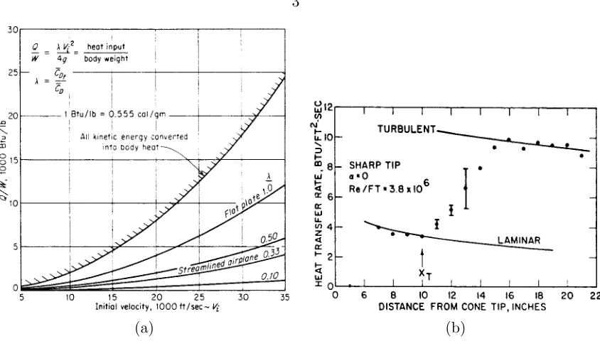
Figure 1.1: Estimated contribution of skin friction (viscous) drag to the overall drag of a hypersonic transport assuming fully laminar and fully turbulent flow. (Reproduced from Reedet al.[92])

The issue of aerodynamic heating is of particular concern in hypervelocity regimes. Figure 1.2a shows the results of a back-of-the-envelope calculation that estimates the total amount of heat transferred to a reentry vehicle assuming different viscous drag fractions. The case of the laminar boundary layer is seen to result in 25% of the heating experienced assuming a turbulent boundary layer. In practice, it is even more important to consider the heat transfer rate to the vehicle since the thermal conductivities of most materials do not allow the heat to be distributed fast enough within the structure to avoid overheating the surface. Figure 1.2b presents results from experiments that show that the heat transfer rate for a laminar boundary layer is 40% less than that of a turbulent boundary layer.

(14)

(a) (b)

Figure 1.2: (a) Estimate of total heat transferred to a reentry vehicle with the viscous drag fraction as a parameter. The amount of heat absorbed assuming a laminar boundary layer (vis-cous drag fraction = 0.10) is seen to be 25% of that for a turbulent boundary layer (vis(vis-cous drag fraction = 0.33). (Reproduced from Dorrance [28]) (b) Experimental data obtained on a sharp cone atM = 5.5 showing that the heat transfer rate for a laminar boundary layer is 40% less than that of a turbulent boundary layer. (Reproduced from Stetson and Rushton [113])

From fish swimming in the sea to the Space Shuttle returning to the Earth, it is clear that the problem of controlling boundary layer transition needs to be addressed. Although sometimes nature can be used as a guide for human beings, this can not always be done and one must then rely on theory and extensive wind tunnel testing.

1.2

Scope of Present Work

(15)

Figure 1.3: Engineering estimates of the heat transfer rates expected on a trans-atmospheric vehicle are found to be more than one order of magnitude greater than those experienced by the Space Shuttle. (Reproduced from Anderson [3], after Tauber [126])

experiments. The objective of this work was to broadly test the theoretical prediction of linear stability analysis that ultrasonic absorption would delay transition in the hyperveloc-ity boundary layer. In order to understand the experiments, however, it is first necessary to understand the concepts of linear stability analysis, its use and limitations, and its role in understanding transition and boundary layer control schemes.

1.3

Linear Stability Analysis

(16)

flat-plate. Schlichting subsequently contributed a series of papers on this topic, and Tollmien contributed a second paper, resulting in a well-developed viscous theory of boundary layer instability. A summary of their work can be found in Schlichting [104]. At the time, this theory was hotly contested and essentially rejected by the scientific community since no experiment had been successful in observing these waves and, more importantly, it was felt that linear theory should have little relevance to transition to turbulence which is a highly non-linear process. This opinion remained unchanged until the ground-breaking experiments of Schubauer and Skramstad [106] conclusively demonstrated the existence of instability waves in the subsonic laminar boundary layer and the theory’s successful quantitative description of their behaviour.

Since then, linear stability theory has been developed extensively. Both theory and experiments have been extended with some success to include compressibility, pressure gra-dients, wall cooling and heating, blowing and suction, and many other effects. A complete review of the present-day knowledge of linear stability analysis is not possible here. In-stead, the basic principles of the analysis will be described and the main results relevant to the present experiments will be discussed. Mack’s review [69] is the most comprehensive and detailed compilation of linear stability analysis to date and includes the derivations for the linear stability equations for both incompressible and compressible flow. Other review articles by Reshotko [96], and more recently, by Reed et al.[93] also provide excellent dis-cussion. Stetson’s article [111] is the most complete review of hypersonic linear stability analysis and boundary layer transition and is the most applicable to the present work.

(17)

problem determines the values of the last four quantities. It is common to perform the analysis using only two-dimensional disturbances, in which case β is taken to be zero. In both cases, the stability of these travelling waves can be determined by examining the sign of the real part of the exponent. A temporal stability analysis is performed by assuming α to be real and allowingω =ω_r+jω_i to be complex. In this case, if the imaginary part of ω is positive then there is unbounded exponential growth of the wave (i.e., it is unsta-ble). An alternative is to perform a spatial stability analysis by assumingω to be real and allowingα =α_r+jα_i to be complex. This time, if the imaginary part ofα is negative then the waves are unstable and will result in unbounded growth of the disturbances.

1.3.1 Incompressible Linear Stability Analysis

Following the steps of linear stability analysis of linearizing the equations of motion and assuming normal-mode disturbances for the case of an incompressible, viscous fluid results in the Orr-Sommerfeld equation; a fourth order linear ordinary differential equation. It was this equation that formed the basis for the work of Tollmien and Schlichting. Taking the limit of this equation as Reynolds number approaches infinity (i.e., the inviscid limit) results in the Rayleigh equation which had been studied extensively by Rayleigh before the turn of the century.

(18)

As indicated previously, since the time of Reynolds, it has been believed that instability waves were related to transition to turbulence. For this reason, early efforts were made to find solutions which reduced the growth rate of the T-S waves. These studies revealed that a cold wall reduced these growth rates and this led to the prediction by linear theory that wall cooling would stabilize the boundary layer. Favourable pressure gradients and wall normal suction were also found to reduce the disturbance growth rates and were also expected to stabilize the boundary layer.

1.3.2 Compressible Linear Stability Analysis

The most significant early attempt to extend linear theory to include the effects of compressibility was performed by Lees and Lin [64]. Their work led to the necessary and sufficient condition of the existence of a generalized inflection point (D(ρDU) = 0, where D is differentiation with respect to the wall normal direction) for inviscid instability. The importance of this generalized inflection point is recognized when one realizes that a bound-ary layer in supersonic flow over an insulated surface always exhibits this inflection point. This implies that all such boundary layers are unstable to inviscid waves.

(19)

Sonic Line:

y

a

p(y)

Acoustic

Rays

U(y)

y

c-U(y

a

) = a(y

a

)

Figure 1.4: Schematic diagram showing the Mack mode in the boundary layer. U(y) is the mean flow velocity profile, p(y) is the disturbance pressure profile, c is the phase velocity of the waves, ais the local speed of sound,y_a is the location of the sonic line (i.e., the location in the boundary layer where the disturbances are sonic relative to the local mean flow velocity). (Reproduced from Fedorov and Malmuth [32])

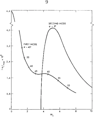
The importance of the second mode (or Mack mode) is seen in Figure 1.5, which shows the maximum amplification rates of the instability waves as a function of Mach number. The maximum growth rate of the first mode is shown to decrease as Mach number is increased. Furthermore, the most unstable first mode frequencies occur for waves that are oblique to the main flow (ψ >0) and must essentially be considered as three-dimensional disturbances (i.e., Squire’s theorem does not hold). This is different from the behaviour in incompressible flows (M →0) where the most unstable waves are parallel to the mean flow. For supersonic flows, the oblique first mode waves are seen to be the dominant mode, and they were found to be stabilized by wall cooling, favourable pressure gradients and boundary layer suction just as in the incompressible case. As Mach number increases, however, the second mode is seen to come into existence and very quickly becomes the dominant instability mode forM >4. This observation, combined with the fundamentally different nature of the second mode as compared to the first mode, led to the conclusion that the problem of hypersonic boundary layer transition must be treated separately from subsonic and supersonic transition. In particular, it was appreciated that any attempt to control the hypersonic boundary layer must directly address the Mack mode. This realization represented a significant advancement in the understanding of boundary layer transition and explained some previously unexplained experimental results.

(20)

Figure 1.5: Results of spatial linear stability analysis for supersonic flow over a cone showing the growth rate of the first and second modes as functions of Mach number. (Reproduced from Mack [67])

(21)

fre-quency of the most unstable mode through the relationf 'U_e/(2δ), wheref is frequency, U_e is the boundary layer edge velocity and δ is the boundary layer thickness. For hyper-velocity flight vehicles travelling at 6 km/s with a boundary layer approximately 10 mm thick, the Mack mode frequency would be approximately 300 kHz.

Once again, because of the recognition of the role of linear stability with respect to tran-sition, a variety of numerical studies were performed to identify regimes that minimized the growth rates of the second mode. It has already been mentioned that Mack had demon-strated that, although wall cooling was a stabilizing influence on the first mode, it was a strong destabilizing influence on the second mode. This effect is of particular importance for hypervelocity flight vehicles where structural considerations require that the wall tem-perature be very small compared to boundary layer temtem-peratures; in essence it is a cold wall. Further work by Malik [70], and Zurigat et al. [136] showed that similar to the first mode, the second mode was stabilized by favourable pressure gradients. In addition, Malik showed that the second mode was stabilized by boundary layer suction. It is only very re-cently that linear stability analysis has begun to include real gas effects that are important at high temperatures. Early work in this area by Malik and Anderson [71] assumed thermal and chemical equilibrium, while later work by Stuckert and Reed [122] considered chemical non-equilibrium (but still thermal equilibrium). Numerical studies by Bertolotti [9] which considered thermal non-equilibrium (but no chemistry) have shown that the assumption of thermal equilibrium is too restrictive and, in fact, vibrational relaxation by itself is desta-bilizing to the second mode. The most recent work, however, by Hudson et al. [50] and Johnsonet al.[51] have included both chemical and thermal non-equilibrium effects. This last study indicates that the use of thermochemical non-equilibrium effects in establishing the mean flow is slightly destabilizing. This, however, is greatly overshadowed by the strong stabilizing effect of having chemistry in the disturbances themselves.

1.3.3 Other Linear Stability Mechanisms

(22)

The first of these, known as cross-flow instability, typically occurs in three-dimensional boundary layers such as those found on swept wings and cones at angles-of-attack. It occurs as a result of an inflection point in the cross-flow velocity profile. Most of the current knowledge relates to low-speed flows and is reviewed by Saric [103]. The most important observation is that these waves are only weakly affected by cooling. Very recent experiments on an elliptic cone by Kimmel et al. [59] and Poggie et al. [88] are the first to study cross-flow instability in hypersonic flow. Their preliminary results indicate that the cross-flow instability may be the dominant instability and the nature of the transition process is quite different from that previously observed on cones and flat-plates.

The other type, known as G¨ortler instability, manifests itself in the form of pairs of counter-rotating vortices produced by concave streamline curvature. Once again, little is known about this instability with respect to hypersonic flows. Although it has not been studied explicitly, knowledge of this instability was recently used to design the first quiet hypersonic nozzle [17]. A review of this instability at lower speeds is provided by Saric [102]. Finally, recent theoretical work by Malmuth [72] suggests another mechanism for wave amplification by the shock layer in the strong interaction region.

1.4

Transition

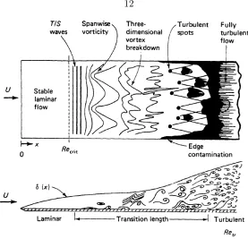
The general process by which transition is believed to occur is shown schematically in Figure 1.6 for the specific case of incompressible flow. A similar process is believed to occur for the second mode, and most likely also for the cross-flow instability and G¨ortler instability mechanisms when they are relevant. Initially, a stable laminar boundary layer exists and all linear instability waves are damped. As the critical Reynolds number is reached, waves of particular frequencies become unstable and experience unbounded growth. The unstable waves grow in amplitude to the point that non-linear processes take over and turbulent spots begin to appear before the boundary layer ultimately transitions to turbulence.

(23)

Figure 1.6: Schematic diagram showing the transition process from the initial linear amplification of instability waves through to the formation of turbulent spots and transition. (Reproduced from White [132])

(24)

compare well with free-flight data [16]. A proper transition experiment must, therefore, not only include Mach number and Reynolds number in its similarity criteria, but also the environmental conditions.

It is important to note that this is the best understanding of how transition occurs. As Stetson [111] observes, there is no transition theory. Linear stability in itself can not predict the onset of transition, rather it simply predicts the unstable growth of waves in the laminar boundary layer. The most common prediction tool used, the so-called eN method by Smith and Camberoni [108], assumes that transition occurs when the amplitude ratio of the most unstable mode reaches a value of eN where N was found to range from 9 to 11 as determined by correlation with experiments. At best, this is a semi-empirical method, where the value of N can depend drastically on the flow configuration, the environment and the exact instability mechanism. Despite this apparent incompleteness, the value of stability theory can not be overstated. It provides valuable information about the processes that lead up to transition and, as alluded to earlier, it provides clues as to how a boundary layer can be controlled.

1.5

Previous Transition Experiments in T5

(25)

the closest to a true stability experiment in the sense that it identifies the formation of turbulent spots and tracks the growth of the transition region.

In addition to capturing a flow visualization (resonantly enhanced shadowgraph) image of the boundary layer transition process, the experiments by Germain and Adam determined the dependance of transition Reynolds number (Re_tr) on specific stagnation enthalpy (h_o). One of the main results obtained by Germain was that the transition Reynolds number correlated with specific stagnation enthalpy provided that the Reynolds number was cal-culated at a reference temperature (Re∗_tr) rather than the boundary layer edge conditions. Furthermore, the Re∗_tr was consistently higher in air than in nitrogen and even still higher in carbon dioxide. This delay in transition for the different gases was attributed to the increased chemical activity acting as a damping mechanism on the growth rate of the in-stability waves. Carbon dioxide has the lowest dissociation energy and a larger number of vibrational modes, and therefore exhibited the strongest damping effect and the greatest increase in transition Reynolds number.

Another interesting result obtained from the experiments was that the flow visualization images seemed to indicate that low frequency waves were present in the boundary layer. This suggested that perhaps the first mode may be the dominant mode. This evidence was not particularly strong, and certainly all theoretical results indicated that the second mode should be the dominant mode. Subsequent linear stability calculations which included thermochemical non-equilibrium effects were performed by Johnson et al. [51] for direct comparison with the T5 experiments. Figure 1.7a shows the computed amplification rates for a typical T5 high enthalpy shot in air with (solid line) and without (dashed line) the effects of vibrational excitation and chemistry, while Figure 1.7b shows the same for a shot in carbon dioxide. The frequencies of the most strongly amplified mode are seen to be approximately 1 to 3 MHz and such high frequencies are highly indicative of the second mode. Furthermore, these calculations showed a strong damping effect of the amplification rates because of vibrational excitation and chemistry. As anticipated from the experiments, the damping effect is seen to be much more pronounced for the carbon dioxide case.

(26)

(a) (b)

Figure 1.7: Results of linear stability calculations with thermochemical non-equilibrium ef-fects for (a) T5 shot 1162 (in air, h0= 9.3 MJ/kg) and (b) T5 shot 1150 (in carbon diox-ide,h₀= 4.0 MJ/kg). The frequencies are seen to be of the order of megahertz which is indicative of the dominance of the Mack mode. The thermochemical non-equilibrium effects are seen to damp the growth rates (solid lines are below the dashed lines), with the effect being more pronounced in carbon dioxide. (Reproduced from Johnsonet al.[51])

mode waves based on the boundary layer thickness. Numerical simulations by Adam [1] (along with approximate measurements made from the shadowgraphs) indicated that the boundary layer thickness ranged from 0.5 mm to 1 mm. The second mode, therefore, has a wavelength of approximately 1 mm to 2 mm at the T5 conditions. Noting that a typical boundary layer edge velocity is about 5 km/s and using the equation f 'U_e/(2δ), the frequency can be estimated purely from the experimental data to be around 2.5 to 5 MHz which also agrees with the linear stability calculations.

(27)

1.6

Boundary Layer Control

As indicated earlier, the desire to control a boundary layer, specifically to extend the laminar region, is of utmost importance in all flight regimes for the purposes of drag and heating reduction. To this end, many boundary layer control schemes have been proposed based on linear stability analysis. For subsonic and supersonic flow, linear stability analysis showed that wall cooling, favourable pressure gradients and suction all had strong stabilizing effects on the growth rates of the T-S waves. These results formed the basis for a variety of wind tunnel experiments and flight tests for subsonic and supersonic flows, although none have been successfully used in an operational environment for a variety of practical reasons. To date, boundary layer control has not been used on any hypervelocity flight vehicle.

(28)

which cross-flow instabilities become important and as noted earlier, these instabilities are not strongly stabilized by wall cooling. An extensive series of experiments and flight tests with an F-94 were performed by Goldsmith [39, 40], Pfenningeret al.[86], Grothet al.[43], and Carmichaelet al. [13, 14] at Northrop Corporation throughout the 1950’s and 1960’s. These same individuals were involved with similar experiments on the NASA X-21. A de-tailed review of this early work can be found in Pfenninger [85]. Subsequent flight research experiments were performed by NASA using an F-111 and F-14 to examine the effects of crossflow. In addition, during the 1980’s, NASA used a C-140 Jetstar to examine the ro-bustness of leading edge LFC with respect to insect, ice, snow and other contamination. More recent investigations into laminar flow control include flight tests on a modified 757 aircraft and on the tail fin of an A320 aircraft [19]. In addition NASA initiated a test program in 1990 to demonstrate the first supersonic LFC using their F-16XL laminar flow control test aircraft [80]. Recent reviews on early and present day laminar flow control computations, experiments and flight tests can be found in Braslow [11] and Joslin [52]. These experiments and flight tests all achieved varying degrees of success, attaining lam-inar flow over significant portions of the wing surface and attaining significant reductions in drag (as much as 5%). Unfortunately, contamination from pollution, insects, icing and other atmospheric conditions limit their effectiveness. These operational issues combined with the increased cost and weight penalty typically prevent the widespread use of such active control techniques.

(29)

1.7

Overview

(30)

Chapter 2

Theoretical Approach

This chapter summarizes the theoretical and computational work that forms the basis for the experiments. It first describes the linear stability analysis performed by Fedorov and Malmuth that predicted the reduction in growth rates of the unstable waves. The physics of the flow are then examined and the validity of the electrical analogy used in the stability analysis is discussed. The fundamental analysis originally performed by Kirchhoff is then presented in order to better understand the details of the mechanism of the attenuation of the unstable waves. Finally, the theory is used to determine the required parameters for the present experiments.

2.1

General Description

As outlined in the previous chapter, it is generally accepted that, in the absence of large flow disturbances, transition of the two-dimensional or quasi-two-dimensional hypersonic boundary layer (M >4) is caused by the amplification of the second mode (Mack mode) which is acoustic in nature. In this case, the boundary layer acts as an acoustic wave guide as high frequency pressure perturbations become trapped in the boundary layer, grow in amplitude, and eventually cause the boundary layer to transition from laminar to turbu-lent. Fedorov and Malmuth postulated that these high frequency acoustic waves could be damped by choosing a suitable ultrasonically absorbing surface, thereby reducing the sec-ond mode growth rate and ultimately delaying transition1. In particular, a ‘porous’ surface with suitably sized cylindrical blind microholes (i.e., holes with closed bottoms) arranged in a rectangular grid was proposed as the ultrasonically absorbing surface. The term ‘porous’ is somewhat of a misnomer since no flow actually passes through the holes. The appro-priate boundary conditions to represent this surface were applied and this hypothesis was successfully tested numerically using linear stability analysis.

1_{U.S. patent number 5 884 871 issued to Boeing, March 23, 1999 (Dr. Alexander V. Fedorov and}

(31)

2.2

Linear Stability Analysis

The complete set of linear stability analyses which formed the basis for these experiments is summarized below and is described in detail in Fedorov and Malmuth [31]. The initial inviscid analysis is also described in Fedorovet al.[33] and the details of the viscous analysis are also presented in Fedorov and Malmuth [32]. These analyses are similar to typical linear stability analyses performed in the past. The innovation by Fedorov and Malmuth is the use of a generic boundary condition to represent the ultrasonically absorbing surface. The even more significant innovation is the development and use of boundary conditions to represent the specified surface microstructure of equally spaced cylindrical blind microholes.

2.2.1 Inviscid Linear Stability Analysis

The linear stability analysis considered two-dimensional supersonic boundary layer flow over a flat plate. The inviscid, compressible stability equations can be derived for linearized, locally parallel, viscous flow of a heat conducting perfect gas in the limit of zero heat conduction and infinite Reynolds number. The details of this derivation are provided in Mack [69]. In general, for compressible linear stability analysis, Squire’s theorem does not hold since the energy dissipation terms in the energy equation do not transform properly from the three-dimensional problem to an equivalent two-dimensional problem. For the inviscid, compressible case, however, these terms are ignored and Squire’s theorem can be used to note that the most unstable disturbances are two-dimensional and are parallel to the mean flow. It is, therefore, adequate to only consider two-dimensional normal-mode disturbances of the form

[˜u,˜v,p,˜ θ˜]T(x, y, t) = [u(y), v(y), p(y), θ(y)]Tej(αx−ωt), (2.1)

whereuandvare the velocity components in thexandydirections,pis the pressure,θis the temperature, the tilde (∼) quantities are the disturbance quantities, α is the wavenumber, and ω is the frequency. The final linearized normal mode equations to be solved are

v?0 = U?0

U?₋_c?v?+jα?

T?₋_M2₍_U?₋_c?₎2

U?₋_c? p?, (2.2)

p?0 =−jα?U

?₋_c?

(32)

whereU?andT? are the mean flow velocity and temperature which are both functions ofy?, Mis the edge Mach number,c?=ω?/α?is the complex wave speed and the primes (0) denote differentiation with respect toy?. The star (?) expressions represent non-dimensional quan-tities that have been non-dimensionalized with respect to the displacement thickness (δ∗), the local boundary layer edge velocity (U_e) and the local edge temperature (T_e). Pressure is referenced to twice the dynamic pressure (ρ_eU_e2) and the wavenumber and frequency are non-dimensionalized by α? =αδ∗ and ω?=ω δ∗/U_e, respectively.

As stated earlier, the difference from the analysis by Mack is in the boundary conditions which are now

v?(0) =A p?(0), p?(∞) = 0, (2.4)

where A is a complex absorption coefficient that depends on the surface properties. An expression for this absorption coefficient remains to be determined. By rearranging the above system of equations, one can derive the following relation for pressure fluctuations

p?00−

µ

2U?0 U?−_c? −

T?0 T?

¶

p?0+λ2p? = 0, λ2 =α?2

·

M2(U?−c?)2 T? −1

¸

, (2.5)

with the boundary conditions

p?(∞) = 0, p?0(0) =Ajα

?_c?

T?₍₀₎p?(0). (2.6)

Using the WKB method, the solution to Equation 2.5 can be expressed as:

p(y) = ˆp?₁(y)e−j

R_y

0 λdy_{+ ˆ}_p?₂₍_y₎_ej

R_y

0 λdy₊_O₍_²₎_, _(2.7)

ˆ

p?₁_,₂(y) =Const₁_,₂U√−c T

·

M2(U −c)2

T −1

¸₋₀_.₂₅

, (2.8)

where ˆp?₁ is the incident wave, ˆp?₂ is the reflected wave from the surface, and²= 1/max(|λ|) is small. The reflection coefficient is defined as

τ = pˆ

(33)

τ= 1

τ= 0.8

τ= 0.6 0.03

0.02

0.01

0

1.1 1.2 1.3 1.4 1.5 1.6 1.7 1.8

α αα α

Increasing transparency Imωωωω

Figure 2.1: Plot of temporal growth rate of the second mode (Im(ω) = Im(ω?)) versus wavenum-ber (α=α?) with the wall reflection coefficient (τ) as a parameter. Decreasing the wall reflection coefficient is seen to have a strong damping effect on the growth rate; Mach numberM=6, specific heat ratio γ=1.4, Prandtl number P r=0.72, and wall temperature ratio T?

w/Taw? =0.2 (typical of

hypersonic vehicles). (Reproduced from Fedorovet al.[33])

and the following explicit form for the absorption coefficient can be obtained

A=−T

?₍₀₎

c?

s

M2c?2

T?₍₀₎ −1

1−τ

1 +τ, Real(A)<0. (2.10)

The original eigenvalue problem defined in Equations 2.2 - 2.4 using the absorption coeffi-cient in Equation 2.10 was then solved using a temporal linear stability analysis. Figure 2.1 shows the results of the numerical integration for a flat plate boundary layer on a cool wall at different values of the reflection coefficient. Recall that for a temporal linear stability analysis the quantity Im(ω) is the growth rate of the wave with positive quantities identify-ing unstable exponential growth. This plot clearly shows the general trend that decreasidentify-ing the reflection coefficient (i.e., increasing the amount of absorption) tends to decrease the growth rate of the most unstable mode.

2.2.2 Viscous Linear Stability Analysis

(34)

Once again, the detailed derivation of these equations is given in Mack [69]. As mentioned previously, it is not possible to simplify this case to a fully two-dimensional problem and it is necessary to consider three-dimensional disturbances of the form

[˜u,v,˜ w,˜ p,˜ θ˜]T(x, y, t) = [u(y), v(y), w(y), p(y), θ(y)]Tej(αx+βx−ωt), (2.11)

whereα andβare the wavenumber components in thexandydirections, respectively. The final linearized normal-mode stability equations represent an 8th_{order system of differential}

equations that can be expressed in the form

d¯z

dy =S·¯z, (2.12)

¯z= [u,du

dy, v, p, θ, dθ dy, w,

dw dy]

T _(2.13)

where S is an 8 x 8 matrix whose coefficients are functions of the mean velocity profiles, the displacement thickness, the Reynolds number, the Prandtl number, the ratio of specific heats, the parameters of a temperature-viscosity law, and the disturbance properties (ω,α, β). The boundary conditions for this problem are

u(0) = 0, w(0) = 0, θ(0) = 0, v(0) =A p(0), (2.14) u(∞) =v(∞) =w(∞) =θ(∞) = 0, (2.15)

whereAis the complex absorption coefficient given in the previous section. The eigenvalue problem 2.12 - 2.15 was solved by Fedorov and Malmuth using a spatial linear stability analysis. Figure 2.2 shows a plot of the growth rate versus Reynolds number for a par-ticular frequency with the reflection coefficient as a parameter. Once again, the trend of strong stabilization with increasing absorption is observed. In fact, for this analysis, the disturbances were completely stabilized at all Reynolds numbers for τ < 0.5.

2.2.3 Viscous Analysis with Porous Microstructure Boundary Conditions

(35)

Figure 2.2: Plot of spatial growth rate of the second mode (σ) versus Reynolds num-ber (R=Re_δ∗ =δ∗U_eρ_e/µ_e) with the wall reflection coefficient (τ) as a parameter. As with the

inviscid case, decreasing the wall reflection coefficient is seen to have a strong damping effect on the growth rate; M=6, P r=0.72, γ=1.4, F?₌_ωµ

e/ρeUe2= 2.78×10−4, Tw?/Tad? = 0.2. The

vis-cosity (µ) was computed using a power lawµ∼T0.75_{. (Reproduced from Fedorov}_{et al.}_[33])

specific surface could be constructed to perform this task. As mentioned earlier, the more significant innovation by Fedorov and Malmuth was to apply boundary conditions that were representative of a surface with specific microstructure. The idea of using a porous surface with equally spaced blind cylindrical microholes has its roots in architectural acoustics where similar surfaces with larger holes sized for audio wavelengths are often used to control the acoustics of concert halls and other similar facilities. The remainder of this section is used to rederive a new complex absorption coefficient A that is based on the specific proposed surface microstructure and to discuss the results of the linear stability analysis performed using this new boundary condition.

(36)

0000000000000

1111111111111 External Boundary Layer

w

Radius (r ) s

h

000000000

111111111

Wall Conditions (w) Edge Conditions (e)

Internal Boundary Layer

Top View

+

Figure 2.3: Schematic diagram showing the porous microstructure under consideration. The holes of radius rw and depth h are arranged in a rectangular grid with a uniform spacing of s. The

‘external boundary layer’ refers to the the overall boundary layer on the surface, while the ‘internal boundary layer’ refers to the boundary layer within a hole.

(37)

relations

Z_o=

r

Z

Y, Λ = √

Z Y . (2.16)

The expressions for the specific impedance and specific admittance must be derived from the actual flow physics and are found to be

Z =−jωρ_w

·

1− 2 k_v

J₁(k_v) J₀(k_v)

¸₋₁

, (2.17)

Y =− jω ρ_wc_w2

·

1 + (γ−1)2 k_t

J₁(k_t) J₀(k_t)

¸

, (2.18)

whereρ_w is the mean density in the tube, c_w is the mean sound speed in the tube,γ is the ratio of specific heats,J₀ andJ₁ are Bessel functions of the first kind, and the subscriptw is used to denote quantities evaluated at the wall of the external surface (i.e., at the input to the microhole). The arguments of the Bessel functions, k_v and k_t, are the ratios of the tube radius to the internal viscous and thermal boundary layer thicknesses, respectively, and can be shown to be

k_v =r_w

s

jωρ_w

µ_w , kt=rw

r

jωρ_wC_p

k_w , (2.19)

where µ_w is the viscosity, k_w is the thermal conductivity and C_p is the specific heat at constant pressure. Note that the viscous and thermal boundary layer thicknesses are related through k_t = k_v√P r, where P r is the Prandtl number. All of the above equations are derived in detail from the fundamental flow physics and appropriate electrical circuit theory in Section 2.3. Using the relation

J₀(x) +J₂(x) = 2J1(x)

x , (2.20)

the following expressions can be obtained:

Z =jωρ_wJ0(kv)

J₂(k_v), (2.21)

Y =− jω ρ_wc_w2

·

γ+ (γ−1)J2(kt) J₀(k_t)

¸

. (2.22)

(38)

thickness (δ∗) and the mean flow parameters at the edge of the external boundary layer, the following non-dimensional expressions can be obtained:

Z?= jω

?

T? w

J₀(k_v)

J₂(k_v), (2.23)

Y? =−jω?M2

·

γ+ (γ−1)J2(kt) J₀(k_t)

¸

, (2.24)

k_v?=r?

s

jω?_ρ? w

µ? w

Re_δ∗, (2.25)

where Re_δ∗ is the Reynolds number based on the external displacement thickness and external boundary layer edge conditions, and superscripts stars (?) are used to denote the quantities that have been non-dimensionalized. Once again, borrowing from the electrical analogy, it will be shown in Section 2.3.2 that the input impedance (Z_i) for the configuration under consideration (i.e., blind microhole) is

Z_i? = p

?₍₀₎

¯

v?₍₀₎ =−Zo? coth(−Λ?h?), (2.26)

where p?_{(0) is the pressure at the entrance to the cylindrical microhole (}_i.e._{, it is equal to}

the pressure at the external wall, p?_w), ¯v?(0) is the average vertical velocity at the entrance to the cylindrical microhole, andh? ₌_h/δ∗ _{is the non-dimensional length of the cylindrical}

microhole. It is this input impedance (or rather its reciprocal which is the input admittance) that is the basis for the absorption coefficient (A) required for the boundary condition to solve the original eigenvalue problem. The above analysis was done for a single hole in the porous surface. The result is extended to the overall porous surface by averaging the vertical velocity ¯v?(0) over the surface area using

v?(0) =nv¯?(0), (2.27)

wheren is the porosity defined as the ratio of the hole volume to the total volume:

n= V olumeHoles V olume_{T otal} =

π r2_w

(39)

wheresis the hole spacing as defined in Figure 2.3. The absorption coefficient then becomes

A= n Z?

i

= n¯v

?₍₀₎

p?₍₀₎ =−

n Z?

o

tanh(−Λ?h?). (2.29)

This is the final expression used in the boundary condition (Equation 2.14) to solve the eigenvalue problem. It is interesting to note that this equation can be further simplified in the case of a deep microhole (h?→ ∞) to

A=− n Z?

o

. (2.30)

(40)

3.5

4.0

4.5

5.0

0.00

0.01

0.02

0.03

0.04

.02

.03

.01

r

=0

σσσσ

R

x10

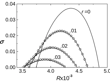
-3

Figure 2.4: Plot of spatial growth rate of the second mode (σ) versus Reynolds num-ber (R=Reδ∗ =δ∗Ueρe/µe) with non-dimensional radius (r) as a parameter. The solid lines

correspond to calculations using both the pressure and thermal admittance boundary conditions and the circles correspond to calculations with the thermal admittance taken to be zero. The caser= 0 corresponds to a solid wall (both pressure and thermal admittance are zero). Increasing the radius of the holes (and therefore the absorption coefficient) is seen to have a strong damp-ing effect on the growth rate; F?_{= 2}_.₈_×₁₀−4_, _n_{= 0}_._5, _M_=6, _{P r}_=0.71, _γ_=1.4, _T?

w/Tad?=0.2 and

h?_{→ ∞}_{. (Reproduced from Fedorov}_{et al.}_[32])

0.0 0.2 0.4 0.6

0.00 0.01 0.02 0.03 0.04

σσσσ

_m

n

0.0 0.1 0.2 0.3

-0.01 0.00 0.01 0.02 0.03 0.04 σσσσ

h

(a) (b)

Figure 2.5: (a) Plot of the maximum spatial growth rate (σm) of the second mode versus the

porosity (n); F?_{= 2}_.₈_×₁₀−4_, _M_=6, _{P r}_=0.71, _γ_=1.4, _T?

w/Tad? =0.2, r?=0.03, and Reδ∗ = 4000.

Increasing the porosity is seen to increase the stabilizing effect. (b) Plot of spatial growth rate (σ) of the second mode versus the non-dimensional depth of the microholes (h=h?_{); all parameters are}

(41)

value and have deeper holes. As indicated by Fedorov and Malmuth [32], the stabilizing effect provided by the porous surface was found to be very robust. In particular, it was found to be effective regardless of the disturbance amplitude and phase distributions in space and time. Furthermore, it was found that it was even more effective at small wall temperature ratios (i.e., cold wall case) typical of actual hypervelocity flight conditions. Calculations using eN-methods indicated that the porous surface was able to increase the transition Reynolds number by more than three times its value without porosity. Such dra-matic delays in transition by a relatively simple passive control scheme would be extremely valuable in reducing heating rates experienced by hypervelocity flight vehicles.

2.3

Flow Physics

The linear stability analysis performed by Fedorov and Malmuth showed great promise for the proposed boundary layer control scheme. The analysis, however, did not give insight into the actual physics of the flow within the porous layer and the manner in which it damped the acoustic perturbations responsible for transition. The boundary conditions were developed using an electrical analogy for propagation of an acoustic wave in a long cylindrical tube which was then averaged over the entire surface to simulate the effect of the many parallel cylindrical holes that made up the porous surface. In order to do this, however, it is important to understand the basis for using the analogy. In the sections below, the electric transmission line equations are derived and the problem of acoustic propagation in a tube is shown to reduce to the electrical equivalent. From this electrical analogy, the details of the flow within each cylindrical microhole can be examined to gain an understanding of the actual mechanism by which the damping occurs. Ultimately, this analogy is related to the more fundamental problem of the attenuation of a single acoustic wave propagating in an infinitely long tube.

2.3.1 Acoustic Propagation in a Tube of Finite Length

(42)

00 00 00 00 00 00 00 11 11 11 11 11 11 11 y x

Zp ZL

0 0 0 0 0 0 0 0 0 1 1 1 1 1 1 1 1 1 L Acoustic Wave Piston

Figure 2.6: Schematic diagram showing the acoustic problem to be solved. A vibrating piston generates acoustic waves which travel back and forth between both ends of the tube. The piston face has an impedance ofZp and the tube end has an impedance ofZL.

tube end which has an impedanceZ_Land the piston face which has an impedance ofZ_p. A critical assumption made in this analysis is that the tube diameter must be much smaller than the acoustic wavelength. The exact definition of ‘small’ will be given in Section 2.3.7. Also, this analysis assumes plane acoustic waves; however, it is not necessary to make this assumption. It can be shown that for tubes of radius much smaller than the acoustic wave-length, any non-uniformities will quickly smooth out and the resulting wave will converge to a plane wave [60, 99]. For a cylindrical rigid-walled acoustic waveguide, Kinsler [60] in-dicates that all waves with angular frequency ω <1.84c/r_w are evanescent standing waves that are attenuated exponentially. This condition can be re-expressed as r_w <1.84λ/(2π). Furthermore, it can be shown that under such conditions, the pressure across the tube is essentially constant.

Before continuing further, it is useful to mention an important difference between acous-tic propagation in an inviscid medium as compared to a viscous medium. When considering the propagation of a plane acoustic wave in the former, it is common to derive the following relation:

P =±ρ_oc_oξ,˙ (2.31)

where P is pressure, ρ_o is equilibrium density of the medium, c_o is the adiabatic speed of sound, ˙ξis the particle velocity and the±is used to denote the forward and backward waves. In this case, the quantityρ_oc_ois often described as being the specific acoustic impedance. In order to include the effects of attenuation, however, the above equation needs to be modified since the relaxation (viscous or thermal) of the medium will introduce a phase lag (φ0−φ) between the pressure and the particle velocity. The above equation is then modified to be

(43)

where W = ρ_oc_oe−j(φ0−φ) is the newly defined specific acoustic impedance. A proper derivation of the above can be found in any acoustics textbook such as Kinsleret al. [60], Morse and Ingard [79] or Pierce [87] and typically involves solving some variation of a lossy Helmholtz equation.

Closely following Rschevkin [99], the solution to the acoustic problem under consid-eration will contain travelling waves in both directions and the particle velocity can be expressed as

˙

ξ(x, t) = [ ˙ξ+(x) + ˙ξ−(x)]e−jωt= (ae−Λx+beΛx)e−jωt, (2.33) where a and b are constants to be determined, ˙ξ+ and ˙ξ− are the forward and backward waves, respectively,ω is the angular frequency,tis time,e−jωt is the assumed time depen-dance, and Λ is the complex propagation constant. The pressure can then be expressed as

P(x, t) =W[ae−Λx−beΛx]e−jωt. (2.34) Using the boundary conditions

Z_pξ˙_i+SP_i =ψ_i (at x= 0), (2.35) Z_Lξ˙_L=SP_L (at x=L), (2.36)

where subscripts i and L are used to denote quantities at the tube entrance (x = 0) and tube end (x = L), respectively, S is the tube cross-sectional area and ψ_i =ψe−jωt is the external forcing function driving the piston,aand b can be determined to be

a= ZL+W S

∆ e

ΛL_ψ, _b₌₋ZL−W S

∆ e

−ΛL_ψ, _(2.37)

∆ = 2[Z_pZ_L+ (W S)2] sinh(ΛL) + 2W S(Z_p+Z_L) cosh(ΛL). (2.38)

The resulting equations are

˙

ξ(x, t) = [(Z_L+W S)eΛ(L−x)−(Z_L−W S)e−Λ(L−x)]ψi

∆, (2.39)

P(x, t) =W[(Z_L+W S)eΛ(L−x)+ (Z_L−W S)e−Λ(L−x)]ψi

(44)

Evaluating the above atx=L, one obtains

˙

ξ_L= 2W S

∆ ψi, PL= 2Z_LW

∆ ψi. (2.41)

Evaluating the same equations at x = 0 and re-expressing the exponentials in terms of hyperbolic functions, one obtains

˙ ξ_i=

·

2Z_L

∆ sinh(ΛL) + 2W S

∆ cosh(ΛL)

¸

ψ_i, (2.42)

P_i=W

·

2W S

∆ sinh(ΛL) + 2Z_L

∆ cosh(ΛL)

¸

ψ_i. (2.43)

Combining Equations 2.41 - 2.43, one can finally express the input pressure and particle velocity in terms of the quantities at the tube end:

˙

ξ_i = cosh(ΛL) ˙ξ_L+ 1

W sinh(ΛL)PL, (2.44)

P_i =W sinh(ΛL) ˙ξ_L+ cosh(ΛL)P_L. (2.45)

An examination of the above equations reveals that they are in the form

˙

ξ_i=C₁ξ˙_L+C₂P_L, (2.46)

P_i=C₃ξ˙_L+C₄P_L, (2.47)

(45)

2.3.2 Electric Transmission Line Theory

For most electrical circuits, the wavelengths of the voltage and current are much longer than the physical size of any actual device and the wave nature can be neglected. This can be readily seen if one considers that for typical 60 Hz electrical power grids, the wavelength is approximately 5000 km. For power transmission lines, however, the length of the con-ducting power line becomes of the same order as the wavelength and it is no longer possible to ignore wave effects. The additional fact that the wavelength is much larger than the cross-sectional diameter of the wire gives reason to believe that this would be an appro-priate analogy for the problem of an acoustic wave propagating in a long, thin tube whose diameter is much smaller than the acoustic wavelength. A detailed derivation and discus-sion of the standard transmisdiscus-sion line equations using basic circuit theory can be found in Karakash [53]. A modified version of this derivation is presented below. Karakash noted that these equations can also be derived from the more fundamental Maxwell equations, although it is unnecessary for the purposes of the present work.

The standard transmission line formalism begins by assuming that a differential segment of the transmission line can be modeled using the circuit diagram shown in Figure 2.7. This is known as a lump-mass model since the electrical properties which are normally distributed along the entire length of the transmission line have been lumped into discrete electrical elements in a transmission line segment of differential length. The series resistance (R) represents the actual resistivity of the wire, the series inductance (L) models phase shifts due to magnetic flux interactions, the shunt conductivity (G) is used to represent leakage current across the dielectric separating the two conductors and the shunt capacitance (C) is used to represent phase shifts due to electric field interactions. The R and G terms are pure resistances and are responsible for losses (attenuation of the signal), while the L and C terms are pure reactances responsible for phase shifts. All of the above quantities are expressed per unit length of transmission wire. Applying Kirchhoff’s current and voltage laws to the circuit diagram, one obtains

i(x+dx, t)−i(x, t) =−(G+jωC)v(x, t)dx, (2.48) v(x+dx, t)−v(x, t) =−(R+jωL)i(x, t)dx, (2.49)

(46)

L/2 L/2 R/2 R/2

C G

V(x,t) V(x+dx,t)

i(x,t) i(x+dx,t)

dx

Figure 2.7: The bottom figure shows the circuit diagram used to represent an electrical transmission line. A differential segment called a ‘T-section’ is removed from the chain and analyzed in order to derive the transmission line equations. The electrical elements (R, L, G,C) are used to represent the various properties and are given per unit length of wire.

distance along the direction of propagation anddx is the unit length of transmission wire. Although not explicitly stated, a time dependance of the forme−jωtis assumed throughout the derivation. Rearranging and taking the limitdx→0, the following differential equations are obtained:

∂i

∂x =−(G+jωC)v=−Y v, (2.50)

∂v

∂x =−(R+jωL)i =−Zi, (2.51)

where Z =R+jωL is the series impedance and Y = G+jωC is the shunt admittance. Differentiating Equation 2.51 and substituting for∂i/∂xfrom Equation 2.50 (and vice versa for the current), one can obtain two uncoupled, second order differential equations:

∂2i ∂x2 = Λ

2_i, ∂2v

∂x2 = Λ

2_v, _(2.52)

where Λ2= (R+jωL)(G+jωC) =ZY. Clearly, the solutions are

i=i+eΛx+i−e−Λx, (2.53)

(47)

where v+, v−, i+ and i− are the arbitrary constants to be determined. Differentiating Equation 2.54 and using it with Equation 2.51, one can show that

i+=−Λ Zv

+_, _i−₌ Λ Zv

−_. _(2.55)

Substituting the above relations into Equations 2.53 and 2.54 and evaluating them atx=L, whereL is the length of the transmission wire, one obtains

I_L=−Λ Z v

+_eΛL₊ Λ

Z v

−_e−ΛL_, _(2.56)

V_L=v+eΛL+v−e−ΛL, (2.57)

whereI_L and V_L are the current and voltage evaluated at the end of the transmission line segment, respectively. Manipulate Equations 2.57 and 2.56, to solve forv+andv−to obtain

v+=−1 2

Ãr

Z

YIL−VL

!

e−ΛL, v−= 1 2

Ãr

Z

YIL+VL

!

eΛL. (2.58)

Substituting back into Equations 2.53 and 2.54, the final equations can be written as

i(x, t) = 1 2

"Ã

I_L+

r

Y ZVL

!

eΛ(L−x)+

Ã

I_L−

r

Y ZVL

!

e−Λ(L−x)

#

e−jωt, (2.59)

v(x, t) = 1 2

"Ãr

Z

YIL+VL

!

eΛ(L−x)+

Ã

−

r

Z

YIL+VL

!

e−Λ(L−x)

#

e−jωt, (2.60)

where the time dependance ofe−jωt has been explicitly stated here for completeness. From these equations, it is clear that the entire system is characterized by Λ = √ZY and Z_o = pZ/Y which are termed the propagation constant and characteristic impedance, respectively. Re-expressing the above equations in terms of hyperbolic functions and eval-uating them at x= 0, the equations become

I_i= cosh(ΛL)I_L+ 1

Z_o sinh(ΛL)VL, (2.61)

V_i=Z_o sinh(ΛL)I_L+ cosh(ΛL)V_L, (2.62)

(48)

equations reveals that they are in the form

I_i =C₁I_L+C₂V_L, (2.63)

V_i=C₃I_L+C₄V_L, (2.64)

where C₁ = C₄ = cosh(ΛL), C₂ = (1/Z_o) sinh(ΛL), and C₃ = Z_o sinh(ΛL). Comparing with Equations 2.46 and 2.47, it is clear that the above equations are identical to those derived for the case of acoustic propagation in a tube. This reduced form of the sym-metric four-pole is useful for deriving some interesting results. For example, the input impedance (Z_i) can be expressed as

Z_i= Vi I_i =

C₃I_L+C₁V_L C₁I_L+C₂V_L =

C₃+Z_LC₁

C₁+Z_LC₂, (2.65)

where Z_L =V_L/I_L is the impedance at the end of the transmission line segment. Substi-tuting the appropriate values into the above equation results in

Z_i = Vi I_i =

Z_o sinh(ΛL) +Z_L cosh(ΛL) cosh(ΛL) + (Z_L/Z_o) sinh(ΛL) =

Z_o tanh(ΛL) +Z_L

1 + (Z_L/Z_o) tanh(ΛL). (2.66)

Consider an open circuit at the end of the transmission line segment (i.e.,Z_L→ ∞) in which case Equation 2.66 reduces to

Z_i =Z_o coth(ΛL). (2.67)