Fields, forces, and flows: What laboratory experiments reveal
about the dynamics of arched plasma structures
Thesis by
Eve Stenson
In Partial Fulfillment of the Requirements for the Degree of
Doctor of Philosophy
California Institute of Technology Pasadena, California
2012
c
⃝2012 Eve Stenson
Except where otherwise noted, this work is licensed under the Creative Commons Attribution-ShareAlike 3.0 Unported License. To view a copy of this license, visit
http://creativecommons.org/licenses/by-sa/3.0/or send a letter to Creative Commons, 444 Castro Street, Suite 900, Mountain View,
Acknowledgements
Mr. Spock: “Under impulse power she expends fuel like any other vessel. We call it ‘plasma.’ But whatever the Klingon designation, is it is merely ionized gas.”
Lt. Uhura: “Well what about all that equipment we’re carrying to catalog gaseous anomalies? Well the thing’s got to have a tailpipe.”
—Stardate 9523.8, figuring out how to detect a cloaked bird of prey (Star Trek VI: The Undiscovered Country)
I used to think plasmas were “merely ionized gas” (though I lacked Mr. Spock’s expertise with plasma propulsion). I had learned back in third grade that there were three states of matter, and when my sixth grade teacher suddenly added another, I was skeptical. Why should some wayward electrons make a gas worthy of being designated a whole separate state? I managed to maintain that skepticism all the way through junior high, high school, and even college. Then, when I was a first year grad student at Caltech, I attended a seminar given by an Applied Physics professor by the name of Paul Bellan, who opened my eyes to how fascinating plasmas can be.
In the years since, thanks to Paul’s expert tutelage and his years of patience, I have become quite the fan of the fourth state of matter, joining the ranks of “scientists who have to explain to friends and acquaintances that they are not studying blood”1[1]. It has been my great privilege and
pleasure to be a part of this research group — to be involved with plasmas and the community of people who study them, both at Caltech and around the world.
From among the ranks of Bellan Plasma Group, I must thank in particular Sett You and Gunsu Yun for being wonderful mentors as well as great officemates. My luck in officemates continued with Bao Ha and Mark Kendall; I have very much enjoyed all of our conversations over the years,
1It is highly gratifying to report that at the time of this writing, the top result of a Google search for the word “plasma”,
both on science and other topics. Other group members with whom I’ve had the honor of work-ing include Shreekrishna Tripathi, Deepak Kumar, Steve Pracko, Rob Moeller, Rory Perkins, Auna Moser, Vernon Chaplin (whom I owe many thanks, as well as many cookies, for all of the comments and corrections he suggested to this dissertation), Zach Tobin, Xiang Zhai — and, more recently, Taiichi Shikama and K.B. Chai. Dave Felt has been an invaluable colleague, above and beyond his building/repairing the electronics systems upon which my research has relied, as have Eleonora Vorobieff, Connie Rodriguez, and Christy Jenstad. I am also indebted to previous group alumni — such as Carlos Romero-Talamas, Freddie Hansen, Scott Hsu, and Mike Brown — who at confer-ences and meetings have been generous with their time and insights, even though their tenures in the group finished before mine began.
My time in graduate school has been very much enriched by my current and former roommates (including Jessie Rosenberg, Neil Halelamien, Matthew Kelley, Tobiko, Plato and Socrates, Xerion, and especially my partner in life, adventures, and so much more, Brian Standley). I have also been lucky to enjoy the companionship of many other amazing people, be it via boba runs with Adam Griffith, board games with Scott Tesmer and Photon, dinners (and more) with the potluck group, diving with PCH Scuba and AAU, Frisbee games, dancing, or the Caltech Y, Alpine Club, CCD, et al. Meanwhile, from three time zones away, my sister Kate and the members of “In/Out” have been an ongoing source of support and friendship.
I would like to thank the Caltech faculty who served on my candidacy and/or defense commit-tees — Ed Stone, Joe Shepherd, Sunil Golwala, and Keith Schwab — for their feedback on my research and/or encouragement. I would also like to thank those faculty from whom I took excellent and valuable courses, as well as others who were simply willing to make time for discussions.
Abstract
Magnetic flux tubes and, more generally, magnetic field structures that link a plasma volume to its boundary are prominent features in plasma systems of significant interest, such as the solar atmosphere and the interiors of magnetic fusion devices.
In order to study the fundamental physics of these systems, experiments were conducted in the laboratory using a magnetized plasma gun to produce individual arched, plasma-filled magnetic flux tubes. More complex plasma topologies were also explored. The absence of confining walls allowed plasmas to evolve freely — which they did, very dynamically, over the course of several microseconds. The experiment setup featured excellent reproducibility, extensive diagnostic ac-cessibility, and several tunable parameters. In particular, a plasma “color coding” technique and magnetic measurements provided new and interesting results.
The single arches or “loops” of plasma exhibited sustained axial collimation, even during a dra-matic evolution from a small, semicircular arch into a kinked structure up to seven times larger. The loops’ magnetic structure was verified as consistent with that of a flux tube, and their evolution was found to be in quantitative agreement with two interrelated magnetohydrodynamic (MHD) theories: a simplified hoop force model for the axis expansion and a recently proposed MHD flow model for the collimation. More complex plasma structures were found to be similarly dominated by the effects of the magnetic field, exhibiting behavior that was highly repeatable but varied significantly from one magnetic structure to the next.
Contents
Acknowledgements iv
Abstract vi
List of Figures xi
List of Tables xiv
1 Introduction 1
1.1 The big picture . . . 1
1.2 Introduction to plasmas . . . 2
1.3 Plasma regimes, especially magnetohydrodynamics . . . 5
1.3.1 Magnetic flux tubes . . . 7
1.3.2 Helicity . . . 8
1.4 The use of laboratory experiments to elucidate fundamental plasma physics relevant to solar and astrophysical phenomena . . . 9
1.5 Overview of this dissertation . . . 10
2 Experiment details 11 2.1 Vacuum system . . . 11
2.2 Magnetized plasma gun . . . 13
2.2.1 History and overview . . . 13
2.2.2 Vacuum magnetic field system . . . 14
2.2.3 Gas delivery . . . 16
2.2.4 Main power system . . . 18
2.3 Diagnostics . . . 19
2.3.2 Current and voltage . . . 20
2.3.3 Magnetic probe array . . . 22
2.3.4 Imaging . . . 25
2.3.5 Dual-gas plasmas . . . 26
2.4 Software . . . 27
2.4.1 Calculations of magnetic field lines . . . 27
2.4.2 Loop-tracing . . . 28
2.4.3 Image processing . . . 30
3 Plasma flows in arched magnetic flux tubes due to MHD forces 33 3.1 Model 1: Simplified hoop force model . . . 34
3.1.1 Derivation for a perfectly conducting circular hoop . . . 34
3.1.2 The “contradiction” of time derivatives . . . 36
3.1.3 Force calculation without constant flux assumption . . . 37
3.1.4 Effect of hoop shape on inductance . . . 39
3.1.5 R(t)predicted by a simplified hoop force model . . . 40
3.2 Model 2: The gobble effect . . . 42
3.2.1 Key concepts . . . 42
3.2.2 Predicted flow velocity . . . 45
3.3 Experiments with single plasma loops . . . 46
3.3.1 Creating arched, plasma-filled flux tubes . . . 46
3.3.2 Visualizing flows with dual-species loops . . . 49
3.3.3 Getting more quantitative with single-species loops . . . 51
3.4 Analysis . . . 54
3.4.1 Hoop-force-driven expansion . . . 54
3.4.2 Gobble-driven flows . . . 58
3.4.3 Complementary forces with comparable scaling . . . 59
3.4.4 Implications for other systems . . . 59
4 Magnetic measurements of individual flux tubes 61 4.1 Measuring the three-dimensional magnetic field . . . 61
4.2 Comparison to a force-free cylinder . . . 68
4.4 Non-force-free current profiles . . . 75
4.5 Summary . . . 76
5 Beyond the individual arched flux tube, more and less 77 5.1 Single loops with unusual vacuum field configurations . . . 77
5.2 Three-footpoint structures . . . 81
5.3 Pairs of loops . . . 82
6 Conclusions and future work 85 6.1 Summary of contributions . . . 85
6.2 A shot illustrating the significance of the magnetic field topology . . . 86
6.3 Future work . . . 87
A Measurements of the vacuum magnetic field 90 A.1 Magnetic flux at the electrode surface . . . 90
A.2 Vacuum field measurements with the magnetic probe array . . . 94
A.3 Calculation of the magnetic field due to a pair of solenoids . . . 97
A.4 Summary . . . 97
B Details of fast gas valve operations 99 B.1 Species-dependent variation in total gas released . . . 99
B.2 Operating regimes . . . 103
B.3 Fast ion gauge measurements of rise time and pressure response . . . 104
B.4 Summary and suggestions . . . 108
C Estimate fordΦ/dtand other circuit parameters 109 D Analyses of uncertainty, variation, and error in loop traces 113 D.1 Method reproducibility . . . 113
D.2 Shot-to-shot variation . . . 114
D.3 Left-handed versus right-handed loop traces . . . 117
D.4 Boundary identification in dual-gas loop traces . . . 120
D.5 Negligibility of viewing angle uncertainty . . . 122
D.7 Summary and discussion . . . 124
E Species variation in single-gas loops 126 E.1 In images . . . 126
E.2 In IV data . . . 127
E.3 In magnetic data . . . 127
E.4 Regarding neon loops . . . 130
F Further adventures in numerical integration 131 F.1 Key issues . . . 131
F.2 The options considered . . . 133
G Alfven speed contours for plasma parameter ranges of interest 135 H Timing survey for single-loop plasmas 138 H.1 Method . . . 138
H.2 Results . . . 139
H.3 Conclusions . . . 143
List of Figures
1.1 Introduction to plasmas . . . 3
1.2 Velocity distribution functions . . . 4
1.3 Cartoon of frozen-in flux . . . 7
2.1 Illustration of the vacuum chamber (with a 5’ graduate student shown for scale) . . . 12
2.2 Views of the solar “quad” gun . . . 15
2.3 Paschen curves for hydrogen, argon, and air . . . 16
2.4 Gas valve; mounting system; power supply output . . . 17
2.5 Main power system grounding setup . . . 19
2.6 Sample IV data . . . 21
2.7 Current traces for H, N, and Ar loops at 4 kV . . . 21
2.8 Views of the magnetic probe array . . . 24
2.9 Unfiltered, 400-nm-filtered, and 656-nm-filtered images . . . 26
2.10 Magnetic field due to a pair of adjacent wire hoops carrying oppositely directed currents 28 2.11 Sequence of traced plasma loop images . . . 29
2.12 Image composite methods . . . 30
2.13 H-alpha- and H-beta-filtered images, combined . . . 31
2.14 10-bit Imacon image . . . 31
2.15 Views of a hydrogen/argon plasma (various image scaling and display options) . . . 32
3.1 A circular hoop with a circular cross section . . . 35
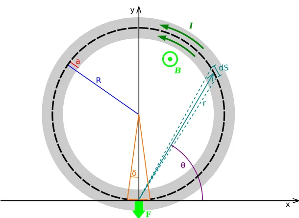
3.2 Diagram for calculating the Lorentz force on a circular, current-carrying hoop . . . . 38
3.3 Collimated plasma arches, in the laboratory and in the solar atmosphere . . . 42
3.4 Cartoon of the gobble effect . . . 43
3.5 Vacuum magnetic field lines; single hydrogen plasma loop . . . 46
3.7 Dual-gas plasma loop traces . . . 49
3.8 Curve length versus time for a number of different dual-gas plasma sections . . . 50
3.9 Loop addition . . . 51
3.10 Dependence of flow speed on current . . . 52
3.11 Numerical derivatives of loop lengths . . . 53
3.12 Example ofIcap(t)with sinusoidal fit . . . 55
3.13 Numerical solutions for the simplified hoop force model . . . 56
3.14 Dependence ofκon ion mass . . . 57
4.1 Magnetic data for single nitrogen loops: left-handed versus right-handed . . . 62
4.2 Sketch, photo, and magnetic field vectors for left- and right-handed nitrogen loops . 64 4.3 Nitrogen loops’ vector fields at earlier times . . . 65
4.4 Evolving plane of magnetic field vectors for a hydrogen loop . . . 67
4.5 Bessel functions and boundary matching . . . 69
4.6 “Taking data” from an infinite, straight flux tube . . . 70
4.7 Flux tube “walk throughs” . . . 71
4.8 Data and model current and magnetic field magnitude versus time . . . 72
4.9 Flux tube model and experimental data . . . 73
4.10 Proposed next refinement for flux tube model . . . 74
5.1 Initial arched plasma for different magnetic field configurations . . . 78
5.2 Magnetic field lines due to a pair of adjacent solenoids energized with the same polarity 78 5.3 Evolution of a plasma with a “half” vacuum field . . . 79
5.4 Ejection of plasma for want of an axial magnetic field . . . 80
5.5 Three-footpoint structures . . . 81
5.6 Pairs of loops of different species . . . 83
5.7 Magnetic fields of loop pairs . . . 84
6.1 Gas released at nozzles outside arched vacuum field . . . 87
A.1 Vacuum field versus time . . . 91
A.2 Properties of the vacuum field in a single-loop setup . . . 92
A.3 Properties of the vacuum field in a dual-loop setup . . . 93
A.5 Measuring the vacuum field with the magnetic probe array . . . 95
A.6 Second set of vacuum field measurements with the magnetic probe array . . . 96
A.7 Magnetic fields calculated for a pair of iron-less solenoids . . . 98
B.1 Gas valve output for hydrogen and nitrogen . . . 100
B.2 Cartoon of particles in a gated reservoir . . . 102
B.3 Fast gas valve output into a test chamber as a function of charging voltage . . . 103
B.4 Current delivered to the fast gas valve from the 400µF capacitor bank . . . 104
B.5 Two versions of the electrical circuit for the fast ion gauge . . . 105
B.6 Time-resolved test chamber pressure . . . 106
B.7 Varying the distance from the gas outlet to the FIG . . . 106
B.8 FIGIeandIcat increasing distances from the outlet . . . 107
B.9 Pressure at increasing distances from the outlet . . . 107
B.10 Pressure calibration for FIG . . . 108
C.1 Sample current and voltage traces . . . 109
C.2 Representative functions forR(t)andI(t). . . 110
C.3 LanddL/dt . . . 110
C.4 dΦ/dt . . . 111
D.1 Five traces of the same hydrogen plasma loop . . . 114
D.2 Shot-to-shot variation in nitrogen and hydrogen loops . . . 115
D.3 Detachment from cathode . . . 116
D.4 Helicity-based variation in loop traces . . . 118
D.5 3D curves modeling plasma loop axes . . . 119
D.6 Measurement uncertainty due to designation of dual-gas boundary . . . 121
D.7 Three helices . . . 122
D.8 Plot ofE(x) . . . 123
E.1 Image differences . . . 126
E.2 IV differences . . . 128
E.3 Magnetic differences . . . 129
F.1 Analytic and numerical solutions for the simplified hoop force model with linear current131
F.2 Numerical solutions’ loop lengths with their first and second derivatives . . . 132
F.3 Numerical solution to full hoop force . . . 133
F.4 Numerical solution without flows . . . 133
G.1 Contour plot of Alfven speeds for hydrogen plasmas . . . 136
G.2 Contour plot of Alfven speeds for nitrogen plasmas . . . 136
G.3 Contour plot of Alfven speeds for argon plasmas . . . 137
H.1 IV properties surveyed . . . 139
H.2 Survey results . . . 139
H.3 Voltage slopes . . . 140
H.4 Additional survey results . . . 140
H.5 “Speedy” optical collimator signals (implying delayed voltage data) . . . 141
List of Tables
2.1 Commonly used static optical filters . . . 26
3.1 Plasma densities calculated fromκ . . . 57
3.2 Neutral gas velocities and ion thermal velocities . . . 58
B.1 Rough estimates of valve outputs for different species, relative to argon . . . 101
B.2 Predictions for gas valve outputs from the simplified Maxwell-Boltzmann model . . 102
C.1 Summary of solar and coaxial gun electrical parameters . . . 112
Chapter 1
Introduction
“If there turn out to be any practical applications, that’s fine and dandy. But we think it’s important that the human race understands where sunlight comes from.”
—Nobel Laureate William Fowler, 1983 [2]
“The sun is a mass of incandescent gas . . .”
—They Might Be Giants, 1993 (“Why Does The Sun Shine?”)
“The sun is a miasma of incandescent plasma . . .”
—They Might Be Giants, 2009 (“Why Does The Sun Really Shine?”)
1.1
The big picture
To those who are unfamiliar with it, “the fourth state of matter” may sound like a creation of science fiction or fantasy authors, akin to “the sixth sense”. To be sure, many authors in these genera do employ plasma-based creations, from radiating life forms to futuristic technologies. Plasma weaponry is a particularly popular option. AndStar Trekaficionados know plasmas have an integral role in the warp drive of a faster-than-light starship — that is, if you believe Gene Rodenberry, the creator of that universe.
composed of plasma. This includes astrophysical jets whose lengths are measured in light years, the diffuse interstellar medium, huge discs of particles accreting around stars or black holes, the stars themselves, and more.
There is one star, of course, with which our planet has a very intimate relationship. Our Sun is plasma through and through, from its core where fusion takes place to its surface covered in arched magnetic plasma structures. Some of the structures are unstable and erupt, sending large quantities of magnetized plasma out into the solar system. If those outgoing solar “storms” encounter Earth, they not only produce dazzling auroras, but can also damage satellites and power grids. Under-standing the physics of what causes eruptions can help us predict and respond to inclement “solar weather.”
Back here on earth, nuclear fusion devices attempt to create plasmas that are hot and dense enough to replicate what happens naturally in the solar core — i.e., produce fusion energy — but without the benefit of a star’s gravity to help with the confinement. One approach to the problem is to corral the plasma in 3D magnetic field configurations — for example, donut-shaped or cruller-shaped toroidal configurations, known as tokamaks and stellerators. At the boundary between the hot, confined plasma and the cool wall of the surrounding metal vacuum chamber are important structures known as divertors.
Both divertors and solar coronal phenomena involve plasmas whose magnetic field lines connect them to a boundary. The physics of these plasma systems can be difficult to capture in computer models, and in some cases, direct measurements of phenomena are complicated or impossible. For-tunately, because the relevant magnetohydrodynamic (MHD) equations for describing magnetized fluids (which will be discussed in detail later in this chapter) have no built-in dependence on the size of the system, we can construct laboratory experiments that experience the same physics, while providing reproducibility, diagnostic accessibility, and some parameter tuning.
Alongside theoretical models, computer simulations, and observations of naturally occurring plasma systems, these experiments allow us to further advance our knowledge of fundamental plasma physics.
1.2
Introduction to plasmas
Figure 1.1: a.) A variety of plasmas are plotted according to their densities and temperatures. The orange star marks the conditions of the plasma experiments described in this dissertation, while the blue star marks Standard Temperature and Pressure (graph c⃝2010 Contemporary Physics Ed-ucation Project, used with permission). b.) A charged particle moving in a uniform magnetic field follows a circular or helical path. It is free to move in the direction parallel to the field, but movement in the perpendicular direction is restricted to the radius of its circle (the size of which depends on its speed in the perpendicular direction). c.) A wire carrying an electric current creates a magnetic field that circles around it.
that the vertical axis, indicating temperature with a logarithmic scale, ranges from 100 to 1,000,000,000 Kelvin. The horizontal axis, indicating density with a logarithmic scale, ranges from103 to1033
particles per cubic meter. The blue star marking the temperature and pressure conditions consid-ered “standard” by chemists and other scientists around the world1lies in bottom right eighth of the graph, where the label reads: “Solids, liquids and gases. Too cool and dense for classical plasmas to exist.” Human beings are far more familiar with the first three states of matter.
In addition to being much hotter and less dense than the first three states of matter, plasmas are also ionized (their defining feature). Some percent of the atoms have lost one or more electrons, resulting in a soup of positively and negatively charged particles, all whizzing around one another.2
Since moving, charged particles are influenced by electric and magnetic fields (Figure 1.1b), and in
1
E.g., the 293 K and2.5×1025m−3specified by the National Institute for Standards and Technology
2
Francis Chen points out that not just any ionized gas can be considered a plasma, since there is a small percentage of ionization in any gas. He defines a plasma as “a quasi-neutral gas of charged and neutral particles that exhibits collective behavior” [3]. Roughly speaking, “quasi-neutral” means that one must zoom in to very small scales (relative to the size of the plasma) in order to find a “chunk” that doesn’t have equal numbers of ions and electrons.
Figure 1.2: a.) Velocity distribution functionsfp+(v)andfe−(v)for ions and electrons, respectively, that have equilibrated at the same temperature. b.) Even within a single species, if there is a source of heating but insufficient collisions to distribute that energy among all the particles, a non-Maxwellian distribution may arise, and the temperature would not be well defined.
turn generate electric and magnetic fields (the latter shown in Figure 1.1c), phenomena emerge that simply do not exist for neutral gases.
The high temperatures, low densities, and ionization can result in conditions quite unintuitive for plasma physics neophytes. Examples, some of which are illustrated in Figures 1.2 and 1.3, include:
• that a plasma with a temperature in the tens of thousands of degrees doesn’t melt the experi-mental apparatus with which it comes in contact (because the energy density is so low);
• that ions and electrons occupying the same volume might be at different temperatures (be-cause interspecies collisions transfer far less energy than intraspecies collisions, due to the difference in mass between ions and electrons); but if they are at the same temperature, the electrons are going much faster than the ions3;
• that the temperature of a species might not even be well defined (because there may not even be enough intraspecies collisions to yield a Maxwell-Boltzmann distribution of velocities), or may not be isotropic (because the presence of a magnetic field is a source of anisotropy);
• that the magnetic field can be thought of as a curious type of rubber band that the plasma may drag, stretch, or even snap.
Note that some of those effects can coexist; others cannot. In short, plasmas yield a very rich (and sometimes confusing) physics. There are many different regimes, and there are infamously many
3
According to the Maxwell-Boltzmann equation, a group of particles with mass m and temperature T have
f(v) = 4/(√π)(m/2kT)3/2v2e−mv2/(2kT) as the distribution function for the magnitude of their velocities. The integral∫v2
different types of waves (each with different components of the plasma vibrating in different ways). Fortunately, there are also plenty of sets of equations to choose from to help sort it all out.
1.3
Plasma regimes, especially magnetohydrodynamics
The most complete description of a plasma involves keeping track of the speed and location of every single particle, and does this for all, say,1020particles in the volume of interest. This would be a rather unenviable assignment: lots of tedium, little opportunity to see the big picture.
Instead, consider “grouping” particles with similar characteristics, and describing the plasma by means of a distribution functionf(x,v, t). (Integrated, this gives the number of particles at timet
with positions and velocities in phase space (i.e., the six-dimensional space ofxandv) between the limits of the integral.) From this starting point, one can use conservation of particles in phase space to derive the Vlasov equation
∂f ∂t +v·
∂f ∂x+
∂
∂v·(af) = 0. (1.1)
The only hitch is that collisions cause particles to appear and disappear in phase space, so in order to take collisions into account the zero on the right-hand side needs to be replaced with a “collision operator” that glosses over the details a bit.
These are the sorts of tradeoffs that one must consider: by making assumptions or glossing over details, equations can be derived that are simpler, easier to understand, and easier to apply. It is a good trade to make, so long as the system to be described is outside the realm where those details are important and those assumptions become untrue. The Vlasov equation would not be a good tool for a system whose interesting physics happens at the level of those collisions, but in all other cases, it works great.
From the Vlasov equation and the distribution function, one can take moments and make ju-dicious assumptions about the time scales of the phenomena being studied to achieve a still more approachable description of the plasma: the two-fluid approach, in which the ions and electrons are mathematically represented not as individual particles, but with each species’ collective qualities: density, mean velocity, pressure, etc. The two-fluid equations relate these quantities and their time and spatial derivatives to one another and to other quantities such as electric and magnetic fields.
densities and velocities in favor of their cumulative density and their relative velocities (i.e., electric current). After integrating over a few more quantities, the result is magnetohydrodynamics. Magne-tohydrodynamics (MHD) is the system of equations for describing a magnetized fluid in terms of its density (ρ), center of mass velocity (U), electric current density (J), pressure tensor (P), resistivity (η), electric field (E), and magnetic field (B).
MHD comprises the continuity equation
∂ρ
∂t +∇ ·(ρU) = 0, (1.2)
the equation of motion4
ρDU
Dt =J×B− ∇P, (1.3)
Faraday’s law
∇ ×E=−∂B
∂t , (1.4)
Ampere’s law
∇ ×B=µ0J, (1.5)
Ohm’s law
E+U×B=ηJ, (1.6)
and a slew of assumptions about the characteristics of the system under consideration. These in-clude assumptions about length scale (large enough that the plasma is quasi-neutral), characteristic velocities (slow relative to the speed of light), relationship between the pressure and density gra-dients (parallel), time scale (longer than the cyclotron periods of both the electrons and ions), and what you’re going to do with Ohm’s law (always take its curl). Yet another approximation — a very useful one, as it turns out — is possible when the resistivity is very low, so that the right-hand side of Ohm’s law can then be set to zero. This is known as ideal MHD.
For plasmas that satisfy all of those assumptions and conditions, ideal MHD is a very good description. For those that don’t, the equations above will not accurately predict or explain the plasma’s behavior, and other equations will be needed. The plasmas created in the Bellan Group are, in fact, primarily in the ideal MHD regime. (It is worth noting, though, that the boundary between different regimes can be surprisingly thin, and plasmas sometimes cross it without warning [4, 5].
4
Figure 1.3: Cartoon of frozen-in flux. When the plasma moves, the frozen-in magnetic flux moves with it, modifying the externally generated magnetic field.
One of the benefits of experiments over computer simulations, though, is that when conditions arise such that the expected mathematical description no longer applies, the system just does something surprising, rather than something unphysical.)
It can be shown that in the limit of zero resistance that defines ideal MHD, the magnetic fluxΦ
satisfies the equation
DΦ
Dt = 0. (1.7)
Since its convective derivative is zero, the flux does not change in the frame of the moving plasma. Rather, the plasma and the magnetic flux move together, as illustrated in Figure 1.3. This is known as the ”frozen-in flux” condition. When it is satisfied, there is a great intuitive advantage to thinking of the plasma in terms of its magnetic topology.
1.3.1 Magnetic flux tubes
A magnetic flux surface is determined by tracing out the path of one or more magnetic field lines. In a toroidal system, such as a tokamak or stellerator, some magnetic field lines close upon themselves after traversing the device a finite number of times; the ratio of times a field line is “wrapped” around the major radius to the number of “transits” along the major radius is given by a rational number. Other field lines never close upon themselves; in this case, the ratio of wraps to transits is irrational. A single, nonclosing field line ergodically fills an entire three-dimensional surface; these are called irrational surfaces. Rational surfaces exist between irrational surfaces and are formed from a collection of infinitely many closed field lines. [6]
character-ized by magnetic field lines linking the boundary to the plasma volume of interest.5 Like a rational surface, an open flux surface is formed from a collection of magnetic field lines, typically chosen based on the symmetry of the system.
Magnetic flux tubes are examples of open flux structures, typically defined by the central axis of a “rope” of twisted magnetic field lines, and they can act a conduit for the transportation of particles and energy between the locations at different ends of that rope. That the flux tube is twisted implies that the curl ofBis finite, so magnetic flux tubes also carry finite current.
Since magnetic fields cause charged particles with velocities perpendicular to the field to un-dergo cyclotron orbits about the direction of the field, these charge carriers are essentially limited to travel along magnetic flux surfaces (to which the magnetic fields are parallel). That is, current flows along flux surfaces.
Depending on the specific orientation of the current and the magnetic field lines, a pressure gradient may exist such that the flux tube is in equilibrium (i.e.,DU/Dt= 0on the left hand side of Equation 1.3). In the case where the current and the magnetic field are exactly parallel, all the terms in the equation of motion are identically zero. This is a “force-free” flux tube. If, on the other hand, there is a finite angle betweenJandB, then this will be balanced in equilibrium by∇P, and the flux tube can be filled with higher density plasma6.
1.3.2 Helicity
Another feature of the flux tube that can be important is whether those twisted magnetic field lines defining the flux tube have a right-handed twist or a left-handed twist. If the twist is right-handed, then the curl of the twist points in the same direction along the flux tube as the magnetic field lines themselves. I.e., current and magnetic field are approximately parallel. If the twist is left-handed, then they are approximately antiparallel. The helicity7 of a magnetic flux tube — and a plasma in general — significantly affects how it interacts with its surroundings. And “the surroundings” of magnetic flux tubes can be quite diverse.
5
A note on terminology: In the solar physics community, the terms “open magnetic field line” and “closed magnetic field line”bothrefer to field lines in the solar corona that connect to the adjacent bounding surface (i.e., the photosphere). The latter return to the photosphere within a solar radius or two, while the former connect to the solar wind, fulfilling the requirement that∇ ·B= 0somewhere far out into the solar system, or beyond.
6In the case of isotropic pressure, the pressure tensorPreduces to the standard gas pressureP. 7
Helicity is actually much more complex than just the handedness of the twist. For one thing, helicity is a scalar quantity, defined asK=∫A·Bd3rfor systems of closed flux. (For open flux systems, gauge ambiguity results in a
1.4
The use of laboratory experiments to elucidate fundamental plasma
physics relevant to solar and astrophysical phenomena
Magnetic flux tubes — and, more generally, magnetic field structures that intercept a boundary — are important to a wide variety of plasma systems. Examples include solar coronal phenomena (e.g., solar coronal loops, coronal mass ejections, and prominences) [7] [8], astrophysical jets [9], spheromak formation8[10], and divertors in magnetic fusion confinement devices [11] [12]. Many of these systems can exhibit rapid dynamic evolutions. Many also pose challenges for computer simulations and/or direct observation.
Computational models often assume reduced dimensionality [13] [14], zero velocity at the boundary [15], and/or periodic boundary conditions [16]. By definition, these models cannot in-vestigate boundary interactions other than those which are assumed. Furthermore, questions have been raised about force-free assumptions [17] often used in solar coronal models, and about the mechanisms for transporting magnetic flux into the corona [14] (another aspect of models that tends to be specified, rather than derived).
While theoretical analyses that assume a force-free state or an equilibrium state are invaluable for situations in which that is indeed the case, they necessarily fail to consider phenomena for which it is not. Many cases of interest involve plasma that is neither uniformly distributed nor stationary. As a result, the rich dynamics of this regime can be difficult to capture.
Direct solar observations also have limitations; coronal events are not reproducible and cannot be measuredin situ. Although advancements have been made in measuring the solar coronal mag-netic field [18, 19, 20], the field is typically calculated from models that assume it is potential or force-free above the photosphere [8]; results differ [21] and may not represent the real system [22]. By contrast, laboratory plasmas are diagnostically accessible and can be highly reproducible, allowing systematic study of configurations where field lines intercept boundaries and exhibit, for example, solar-like dynamics [23]. In addition to work at Caltech, such experiments are in operation at Los Alamos National Laboratory [24], UCLA [25], and Princeton Plasma Physics Laboratory [26], to name a few.
8
1.5
Overview of this dissertation
This dissertation, of course, is about the progress that has been made at Caltech toward this end. To facilitate future reference to the data presented herein, shot numbers are typically included in cap-tions. To facilitate recognition of symmetries and other important features, plasma loop images are rotated to be apex up — except in discussions of the experiment setup. (Gravity is not a factor in the loops’ evolution, but human perception is strongly biased by human eyes’ horizontal orientation.)
Chapter 2
Experiment details
“Experiment can simulate computation: Resolves all scales, includes all correlations, includes all MHD and kinetic effects, “CPU time”<1 second.”
— presentation by physicist Stewart Prager (CMPD/CMSO plasma winter school, 2008)
This chapter describes the experiment setup at Caltech used to create all of the laboratory plas-mas that are the topic of this dissertation.
The setup comprised a modestly sized, pulsed-power, magnetized plasma gun; installed in a much larger vacuum chamber; outfitted with a varied — and ever-changing — collection of di-agnostics. A fiber optic timing system handled all of the experiment triggers. High-speed data acquisition and several types of computer software were used to acquire, process, and analyze the data.
The resulting plasma structures were typically tens of centimeters in size, and with lifetimes measured in microseconds.
2.1
Vacuum system
The stainless steel vacuum chamber is a total of 2 meters long and 1.5 meters in diameter, making it considerably larger than the plasma. As a result, the plasma effectively exists in a “half infinite space”. This is in contrast to plasma confinement devices that traditionally have a conducting wall very close to the plasma (in order to suppress instabilities and maintain steady state operation), and it allows the plasma to evolve dynamically in the ways it “sees fit” to do.
Figure 2.1: Illustration of the vacuum chamber (with a 5’ graduate student shown for scale). The inset shows three viewing angles commonly used for photography and spectroscopy of the plasma. (3D model of the vacuum chamber input to Google SketchUp by Gunsu Yun)
(visible through the first window). The figure inset illustrates common viewing angles for the ex-periment’s high-speed cameras and spectroscopic lines of sight.
The vacuum chamber is typically maintained at a pressure of5×10−8to3×10−7 Torr. The vacuum system is oil-free, so pump oil will not contaminate the chamber. When pumping the chamber down from atmospheric pressure, a Varian Megasorb pump is used down to about 100 mTorr, after which a cryopump1takes over, achieving and maintaining high vacuum. The cryopump is connected to the large port on the bottom of the chamber via a gate valve. The gate valve is used to isolate the chamber from the pump for such purposes as regenerating the pump without bringing
the chamber up to atmosphere, measuring gas valve output via pressure increase in the unpumped chamber, and protecting the pump in the event of an unexpected vacuum break.
A Tribodyne pump is used to evacuate the gas lines for the magnetized plasma gun before each set of experiments (prior to their being filled with the gas species of choice for that set). The same pump is also used to evacuate the cryopump after it has been regenerated.
2.2
Magnetized plasma gun
2.2.1 History and overview
The magnetized plasma gun used for these experiments is the fourth “solar” gun at Caltech. It was first installed in the vacuum chamber in 1999 by Freddy Hansen, and was described in detail in Chapter 5 of his thesis [27]. Modifications have been made to its gas and main power delivery systems since, but much of the operation has remained the same.
Its Mark I and Mark II predecessors were installed on the chamber from 1996 to 1997 and 1997 to 1999, respectively. The Mark III gun, similar to the Mark II and originally built to be used in tandem with it, was not deployed until 2011, when it was installed on a smaller vacuum chamber added to the lab that year. A fifth gun is currently under construction; it is scheduled for installation on the main vacuum chamber in 2012, in place of the Mark IV gun.
A different model of plasma gun is located on the opposite end dome of the main chamber. This model has eightfold radial symmetry, with an inner circular cathode and an outer annular anode. Essentially a coplanar spheromak gun2, it was installed on the chamber in 2001 by Scott Hsu [28]. It replaced a coaxial spheromak gun installed in 1998 by Jimmy Yee [29]. A second coplanar gun was recently installed on the small chamber, opposite the Mark III gun, by Vernon Chaplin.
Thus, by the end of 2012, eight different plasma guns will have been operated in the Bellan Group laboratories over the years.3 For the most part, all of these guns operate by the same basic sequence:
1. Establish a vacuum magnetic field.
2. Release neutral gas in the vicinity of the magnetic field lines.
2
As mentioned in Chapter 1, spheromaks are an “innovative confinement concept” for fusion energy and take advan-tage of the plasma’s tendency to self-organize.
3The addition of the smaller vacuum chamber allows a maximum of four guns to be installed and ready for use at
3. Apply high voltage across the magnetic field lines to ionize the gas.
The geometry of the gun and the specifics of these three elements, however, yield highly disparate plasmas that may undergo very different physical processes.
The current (Mark IV) gun is shown in Figure 2.2. It is sometimes called a “quad gun” due to the outward fourfold symmetry; the copper electrode at the front of the gun is a circle divided into four quarters, and behind each electrode is an identical set of components. When the main power supply is connected, though, the gun is at most bilaterally symmetric. For all the experiments described there, the top two quarters are electrically connected to one another, together forming a cathode; the bottom two quarters compose the anode.
There is one opening in each quarter of the electrode through which gas may be released into the chamber. Coaxial with each gas nozzle is a coil that can be pulsed to produce a vacuum magnetic field (also known as a “potential field” or a “stuffing flux”).
2.2.2 Vacuum magnetic field system
The four magnetic field coils are pulsed with the same two electrolytic capacitor banks that were installed by Hansen. Each bank is equipped with a fast charging unit for convenience. One bank energizes either or both of the two top magnetic field coils. The other bank energizes either or both of the two bottom magnetic field coils.
Each coil can produce a magnetic field pointing in toward or out from the vacuum chamber. This polarity is determined by the polarity with which the coil leads are attached to the capacitor bank cables; switching the leads reverses the direction current flows through the coils and the resulting magnetic field. The leads to a coil can also be detached completely.4
The typical magnetic fields produced have a magnitude of 0.3–0.4 T, measured at the electrode surface directly in front of the coil/nozzle axis, and a lifetime on the order of milliseconds. Thus, they are unchanging on the time scale of a microsecond plasma shot. Detailed measurements (of which there are several) of the spatial and temporal properties of the vacuum field, and how they vary with capacitor bank charging voltage, are described in Appendix A.
By adjusting the charging voltage, energizing a different selection of the coils, and/or switching coil polarities, one can create a variety of different magnetic field configurations that in turn guide different plasma structures.
4
a.) b.) c.)
d.) e.) f.)
Figure 2.2: A collection of views of the solar “quad” gun: a.) Electrode dimensions
b.) Photograph of the electrode (focused on the “near” half, as defined by proximity to the side of the chamber from which the plasma is photographed), with an arm that houses an array of magnetic probes in the foreground. This was taken from inside the chamber with a slightly wide-angle lens. (The ceramic bolt covers at the top and bottom of the photo are, in fact, parallel.)
c.) CAD drawing of the internal components of the gun and its position in the vacuum chamber port (created by Paul Bellan and included here with permission). Green sections are magnetic field coils. Red sections are iron. The long, central structures outlined in black are gas lines.
d.) Illustration of the gun, when configured to make a single hydrogen plasma loop; the purple arches represent the vacuum magnetic field lines (though they are not to scale).
e.) A single hydrogen plasma loop, photographed through the first window, just as it reaches the arm of the magnetic probe array.(shot 5772)
The most straightforward setup is to energize a pair of vertical coils with opposite polarities (Figure 2.2d). The resulting field is akin to that of a horseshoe magnet, and may be parallel or antiparallel to the direction of the current, which flows from anode on the bottom to the cathode on the top. When the two are parallel, the plasma will have right-handed helicity; when they are antiparallel, it will have left-handed helicity. These individual loops of plasma are the topic of Chapter 3; an example is shown in Figure 2.2e.
To make a pair of plasma loops, as shown in Figure 2.2f, four coils are energized. This can be done in such a way that two loops have the same handedness (both right or both left) or the opposite handedness (one of each). These are called cohelicity and counterhelicity setups, respectively, and are discussed in Chapter 5, along with other, more “exotic” magnetic field structures.
It is important to note that the correlation between the vacuum field structure and the plasma structure can vary from being very high to quite low, depending on the extent to which the vacuum field is “compatible” with the requirements for plasma breakdown and current conduction — i.e., the presence of neutral gas.
2.2.3 Gas delivery
When high voltage is applied to the electrodes, breakdown occurs via an avalanching of electrons, starting with a few stray “primary” electrons that are accelerated from cathode to anode by the electric field. These electrons can ionize neutrals via collisions, provided they both A.) can gain sufficient energy between collisions, and B.) encounter neutrals before encountering the anode.
Therefore, in order to produce a plasma, neutral gas must be present at an appropriate density in the vicinity of the electrodes of the magnetized plasma gun at the time that high voltage is applied
across the electrodes. (In most cases, this is equivalent to the gas being in the vicinity of the arched vacuum magnetic field lines that stretch from one gas nozzle to another.) This requirement is known as the Paschen criterion. More precisely, it states that the voltage required for breakdown is a function of the productP d whereP is the pressure of the gas and dis the distance between the electrodes. This function has the form
Vmin(P d) =
BP d
ln (P d) +C (2.1)
whereBandCare constants that are different for different species of gas [10]. Examples of Paschen curves are shown in Figure 2.3.
In order to satisfy the Paschen criterion without filling the chamber with neutral gas (in opposi-tion to the goal of letting the plasma evolve into a vacuum), gas is supplied to the gun by means of two fast gas valves powered by a pulsed power supply.
Figure 2.4a shows a diagram of the gas valve interior. When the gas valve is closed, the alu-minum diaphragm is held against the o-ring underneath it by a combination of the spring and the “back pressure” of the gas supplied to the valve. Gas can flow around the diaphragm into the plenum, but not into the outgoing gas line. To open the valve, a current pulse from the power supply is sent through the coil of wire, inducing a mirror current in the diaphragm and generating a repulsive force
between the two. The diaphragm jumps up, opening the valve briefly before the spring and/or back pressure pushes it closed again. Gunsu Yun estimated that about one fifth of the molecules in the plenum escape [30], but this depends on the species of the gas and the back pressure.
In 2006, two gas valves of the design in Figure 2.4a were installed on the quad gun, in place of the single older model valve put in by Hansen. The new setup, shown in Figure 2.4b, makes it possible for two different species of gas to be used to make the same plasma, either as two halves of the same loop (Chapter 3) or as two single-gas loops, one of each species (Chapter 5).
The new gas valve power supply, built by Dave Felt, allows the two valves to be triggered individually, so as to accommodate the different sound speeds of different neutral gases and, hence, different travel times between the valves and the gun. It contains two 50 µF capacitors, one for each valve; both charge off a single charging supply, but a second supply could be added to allow the valves to be triggered from different voltages. Shreekrishna Tripathi measured the current pulse height as a function of charging voltage and found it to be very linear (Figure 2.4c). Rory Perkins measured the total amount of neutral gas released per valve per pulse, and found it to be about half that of the previous valve that supplied all four nozzles5.
More details about gas valve operation can be found in Appendix B.
2.2.4 Main power system
High voltage is supplied from a 59 µF capacitor that is charged to 3–6 kV, then connected to the electrodes via a krytron-switched ignitron and low-inductance cables. The preset timing program ensures that the resulting electric field is set up only after the vacuum magnetic field has been established and neutral gas is present in the vicinity. (An extended description of the timing system, which is shared with the spheromak experiment, is given by Yun [30].)
Breakdown occurs by means of the electron avalanche process discussed in the previous sec-tion. This process occurs over one to several microseconds and varies from shot to shot, creating a “jitter” in the time between the application of high voltage and the sequence of steps in the plasma’s evolution (which in most cases is very repeatable once initiated). The capacitor then acts as a cur-rent source [31], driving a curcur-rent through the resulting plasma structure (among other paths). A detailed discussion of the current and voltage profiles can be found in the next section.
5This measurement was taken at back pressures of 60 psi for argon and nitrogen and 100 psi for hydrogen. It may be
Figure 2.5: Main power system grounding setup, as updated in 2005. (diagram by Dave Felt and Shreekrishna Tripathi; used with permission)
The main power system was repaired/improved in 2005 by Dave Felt and Shreekrishna Tripathi after a short developed in the high-voltage charging supply. An Ultravolt 10 kV supply was installed in place of the faulty unit, and the grounding of the experiment was updated to the setup shown in Figure 2.5.
2.3
Diagnostics
2.3.1 System overview
The vacuum chamber is outfitted with a suite of diagnostics, many of which can be used for either the solar gun or the spheromak gun. Those that are featured prominently in this dissertation are described in detail below. Other available systems include (but are not limited to):
• a 12-channel, high-resolution (∼5pm/pixel) spectroscopic system [30];
• a set of four x-ray photodiodes, three of which are filtered for specific energy ranges (15–62 eV, above 83 eV, above 200 eV) [32];
• a VUV (vacuum ultraviolet) to soft x-ray (SXR) pinhole camera [31];
• an array of broadband EUV (extreme ultraviolet) vacuum photodiodes [32];
Many of these systems are connected to a VME data acquisition system6, which has 96 channels and is typically run at a 100 MHz sampling rate. Once started, the system takes data continuously until it receives a “stop” signal, at which point it reports the most recent 217samples per channel with a range of 12 bits per sample — i.e., the last 1.3 ms. Thus, the VME can be triggered off the main timing system used for experiment triggers and still capture all of the data (and more), regardless of the microsecond jitter due to breakdown variation.
Other diagnostics that are more sensitive to that jitter, such as the spectrometer and various imaging systems, were triggered off a second, parallel timing system. This system is a clone of the first, but is initiated by light from a collimator aimed at the electrodes, allowing the diagnostic timing system to be triggered by the formation of the plasma itself. For nearly all applications (the exceptions being studies of the very early times in plasma formation before emission is high enough to trigger the collimator), this is preferable because it allows data from one shot to be almost perfectly synchronized or given a predetermined offset relative to the data from another shot.
2.3.2 Current and voltage
The high-voltage capacitor is equipped with a Rogowski coil that was used to measure its output cur-rent. A Tektronix P6015 high-voltage probe was used to measure the voltage across the electrodes. The current and voltage signals were then transmitted to the VME through an optical transmitter and receiver7, for purposes of electrical isolation.
Sample data are shown in Figure 2.6 for a 4 kV, single-loop hydrogen plasma. Note that the voltage trace has a near-constant slope during the lifetime of the plasma loop (the 5µs or so after breakdown). This feature is an artifact of an isolation transformer in the circuit between the optical receiver and the VME; this element was added to eliminate a ground loop but resulted in perfor-mance limitations at lower frequencies [32]. In fact, the voltage remains nearly constant during this time period. This was demonstrated by Xiang Zhai, who recently built a new high-voltage probe that is optically coupled and totally isolated from earth ground.
Because the capacitor acts as a current source, currents during early times tend to be the same to within 10 percent, even for different species; an example of this is shown in Figure 2.7. There are indications, however, that most of this current does not actually flow through the bright, clearly defined plasma structure.
6
Components of the VME system are: eight 12-channel DAQ boards (SiS GmbH SIS3300), one control board (SIS3820), and accompanying computer control code that interfaces with IDL.
Figure 2.6: Sample IV data for a 4 kV single-loop hydrogen plasma. Smoothed current and voltage traces are shown in light red and light blue, respectively, while unsmoothed traces are shown in the darker colors. Smoothing was done with a boxcar average. The vertical dashed line indicates breakdown time, according to the optical collimator signal. Time is given relative to the entire VME data set.(shot 9090)
Magnetic measurements of single plasma loops (detailed in Chapter 4) find the magnetic field peak magnitude to be 0.1–0.2 T, with the “sine-like” components peaking at 200–350 G. Ampere’s law tells us that at the edge of a current channel of radiusA,
Bazimuthal=
µ0I
2πA = 1750 to 3500G (2.2)
forI = 35kA andA=2–4 cm. This implies that only about one tenth — and at most one fifth — of the total current output from the capacitor flows through the loop. Similar values can be calculated from magnetic measurements of the spheromak gun plasmas [33, 31], which are measured with a different set of diagnostics.
The hypothesis that only a fraction of the capacitor current flows through the plasma loop is also consistent with the continued ringing of the current even after that loop detaches or is otherwise disrupted. (The elimination of that current path — with its associated resistance and inductance — does not typically appear to impede the overall current flow, nor correspond to an increase in the magnitude of the voltage across the electrodes.) Calculations for the change in magnetic flux due to plasma loop expansion also suggest loop currents on the order of kA, rather than tens of kA (Appendix C).
Somewhat surprisingly, though, the highly consistent scaling of loop evolution with output cur-rent (which will be discussed in Chapter 3) seems to suggest this fraction is consistent across differ-ent plasma species and differdiffer-ent output currdiffer-ents.
2.3.3 Magnetic probe array
The principle of a “B-dot” probe is straightforward: when the magnetic fluxΦthrough the center of a coil of wire changes, an electromotive forceE is induced in the coil according to Faraday’s law:
E=−NdΦ
dt =−N
d dt
∫
S
B·dA (2.3)
whereN is the number of turns in the coil,S is the surface encompassed by a turn, and Bis the magnetic field through the infinitesimal section of that surfacedA. If S is flat and small enough relative to the scale of the magnetic field thatBis approximately constant over the entire surface, then this reduces to
E =−N AdB⊥
which can be integrated to findB⊥(t), the time-dependent component of the magnetic field perpen-dicular to the coil surface, as a function ofE(t).
Hence, by integrating the voltage measured across the ends of a tiny coil past which a plasma is passing with its frozen-in flux (therefore causing the coil to “see” a changing flux), one can measure the plasma magnetic field normal to that coil. By using three orthogonal coils, one can measure the three-dimensional magnetic field.
A 12-channel probe array was built, installed, and calibrated by Shreekrishna Tripathi, using commercial chip inductors, based on the design by Carlos Romero [34]. The 12 channels are ar-ranged in four clusters of orthogonal triplets, mounted in a plastic tube, which is then housed in a 1 cm quartz tube. This assembly is attached at a 90 degree angle to a metal tube extending from the same end dome as the gun. (This setup allows the probe array to be moved in toward or away from the electrode, as well as rotated in the plane parallel to the electrode.) The signals from the inductors are conveyed to the VME via BNC cables, and thence to the IDL routine that integrates them numerically.
Figure 2.8 provides several views of the magnetic probe array and its orientation relative to the electrode. In order to calculate the probes’ location in space, one must also know:
• that the probe arm rotation point is located43.7±0.4cm from the center of the electrodes, at a 23 degree angle below horizontal8, and
• how far from the electrode the probe arm is extended.
The vacuum fittings for the metal tube and the curvature of the end dome limit the probe’s travel toward the electrode; the closest it can get is 9.5 cm. It can be moved out away from the electrode many tens of centimeters, and/or rotated up and out of the plasma entirely.
The three orthogonal directions measured by the probe array system areBr,Bθ, andBz, using
the natural cylindrical coordinate system of the rotating probe arm. (One must be careful, however, not to confuse these with the coordinates relative to the cylindrical symmetry of the chamber.) Since therθzcoordinate system rotates with the probe arm, it is preferable to express measured magnetic fields in terms of the Cartesian coordinate system with its origin at the center point of the electrodes,
zpointing into the chamber, andxandy being the horizontal and vertical axes, respectively. The magnetic fields measured by the probes in clusternare then written
Bxn=Brncosθ−Bθnsinθ
Byn =Brnsinθ+Bθncosθ (2.5)
Bzn=Bzn
whereθis the angle of inclination from horizontal. These measurements are associated with location
xn=−40.2 +lncosθ
yn=−17.2 +lnsinθ (2.6)
zn=z >9.5
where distances are in centimeters andln=[46.3, 44.3, 42.3, 38.3] is the distance from the rotation
point of the arm to the midpoint of cluster [1, 2, 3, 4], respectively.
2.3.4 Imaging
Because the plasma lifetime is only on the order of microseconds, meaningful images can only be captured with ultra-high-speed cameras. Three cameras were employed for this work:
Imacon 200: This camera9uses an eight-way optical beam splitter to send incoming light to eight
high-resolution microchannel plate image intensifiers, each gated with high-speed electronics and coupled to a CCD. Exploitation of a fast charge transfer process allows each intensified CCD to record a second image in quick succession, allowing the system to capture up to 16 frames in less than a microsecond. The images have a 10-bit dynamic range and a 1200 x 980 resolution.
Princeton Instruments cameras: These two identical single-frame, Peltier-cooled gated ICCD cameras10 are mounted on the same stand, perpendicular to one another. Placing a 50/50 beam splitter at the intersection of their lines of sight enables two captures of the plasma from a single perspective. (This can be used to take simultaneous images using different optical filters, or for cre-ating a two-frame “movie”.) Alternately, placing a mirror a few inches offset from the intersection creates parallel lines of sight that can be used to generate 3D pictures. The images have a 16-bit dynamic range and a 576 x 384 resolution.
9DRS Technologies
wavelength (nm) bandwidth (nm) transmission (%)
400 10 50
480 10 46
485 10 50
656.5 1.2 45
Table 2.1: Commonly used static optical filters
Due to its ability to capture short movies of each individual plasma shot, the Imacon is the workhorse11 of the Bellan plasma lab’s main experiment chamber. It is not particularly suitable for quantitative studies, though, due to its signal-to-noise ratio and a variable relative gain among the CCDs that is different each time the camera is powered up. For quantitative measurements, the Princeton cameras’ low noise and high dynamic range are ideal; they are also often deployed to capture a second perspective of the plasma in addition to Imacon view.
Typical imaging is done with exposure times of 10–100 ns (depending what lens and whether any optical filters are being used) and an interframe time of 200–400 ns.
2.3.5 Dual-gas plasmas
Creating a plasma from two different species of neutral gas has turned out to be a valuable diagnostic technique. Because different atoms have different atomic transitions, optical filters can be used to selectively image the different plasma species, enabling different sections of the plasma to be tracked from frame to frame. Furthermore, because the experiments are highly reproducible, filtered and unfiltered images can be taken of separate shots and then used together. Figure 2.9 illustrates this with an Imacon frame from three different shots, two with optical filters.
In addition to the static filters listed in Table 2.1, the recent purchase of a VariSpec liquid crystal
Figure 2.9: Unfiltered, 400-nm-filtered, and 656-nm-filtered images of nitrogen/hydrogen single loops.(shots 5019, 5027, 5024)
tunable filter with a 7 nm bandwidth enables a filtered image to be obtained for any wavelength in the visible range.
2.4
Software
As mentioned previously, IDL plays a key role in the acquisition, processing, analysis, and presen-tation of data from the VME. It has been used to write programs for several other tasks related to the plasma experiment.
2.4.1 Calculations of magnetic field lines
Because the topology of the vacuum magnetic field generated by the gun has such an incredibly important role in the dynamics of the plasma, and because the gun can be operated with such a variety of coil configurations, a program was written that calculates magnetic field lines due to the presence of one or more circular current-carrying wires.
The user specifies the number, radius, current, and locations12of the wire hoops, as well as the starting points for any magnetic field lines that are to be drawn. The paths of the field lines are then calculated via the fourth-order Runge-Kutta method13[35]:
sn+1 =sn+
h
6(k1+ 2k2+ 2k3+k4) (2.7)
wheresnandsn+1are adjacent points along the field line,his the step size between adjacent points,
andk1throughk4, defined as
k1 =
B(sn)
|B(sn)|
k2 =
B(sn+h2k1)
|B(sn+h2k1)|
k3 =
B(sn+h2k2)
|B(sn+h2k2)|
k4 =
B(sn+hk3)
|B(sn+hk3)|
12
The hoops’ axes of symmetry are all oriented in the same direction, though if there were a need for arbitrarily oriented hoops, this could easily be modified. A stack of coaxial loops can be used to estimate the field of a coil.
13
Figure 2.10: Magnetic field due to a pair of adjacent wire hoops carrying oppositely directed cur-rents
are essentially “samples” of slopes in the vicinity of the direction the magnetic field is going (of which a weighted average is taken for the actual “jump” to the next point).
The program successfully produces closed field lines for reasonable step sizes. These can then be plotted in such a way as the user finds enlightening, projected onto various planes, and so on. Figure 2.10 shows an example for a pair of adjacent coils.
2.4.2 Loop-tracing
In order to quantify and compare the evolution of individual plasma loops, IDL routines were written to facilitate image tracking of the loop axis. One routine displays each image in the series taken by the Imacon camera, asks the user to trace out the location of the axis, and records the resulting mouse clicks. Figure 2.11 shows a typical set of traced loop images.
Figure 2.12: The same shots from Figure 2.9, illustrating various image combination methods. First, the red-filtered shot was a.) subtracted from or b.) averaged with an unfiltered shot. Next, both the red- and blue-filtered shots were either c.) subtracted from or d.) averaged with the unfiltered shot. Finally, since averaging or subtracting multiple shots darkens images, the examples from (c–d) were brightened in the GNU Image Manipulation Program to yield the images in (e–f), respectively.
2.4.3 Image processing
IDL was also used to create color images of the plasma from the grayscale camera photos, via color composites, color tables, and various scaling schemes for each of these.
Composites were made from two or more images taken with or without different optical filters, as was done for the dual-gas plasmas in Figure 2.9. There are infinitely many different ways the ma-trices of pixel values representing the images can be combined. Some of the more useful examples include (in no particular order)
• colorizing an unfiltered image with a filtered image by subtracting the filtered image from one or more of the color channels of the unfiltered image (where the latter was converted to, say, a black and white RGB image),
• combining the same two images by averaging the filtered image with one or more of the channels of the black and white image,
• using one of the above methods, but with one unfiltered and two or more filtered images,
Figure 2.13: A composite of two filtered images of a hydrogen loop, using the H-alpha and H-beta filters.(shots 5778 and 5780)
• using weighted averages or otherwise scaling matrices depending on how bright the source images are,
and many more. Some examples are shown in Figure 2.12. Of course, the same techniques can also be applied to multiple images of single-species plasmas taken at various wavelengths, such as the hydrogen loop in Figure 2.13.
While quantitative studies with the Princeton camera have been done, in which pixel values are measured precisely and emission ratios are estimated based on the properties of the different filters that were used, making composite images is usually a matter of finding the most suitable settings to faithfully and effectively communicate the information about the plasma contained in the camera images. Different image combination methods may highlight different parts of that information, while both still being valid.
Even when only unfiltered images have been taken of a particular plasma, there are image pro-cessing questions such as how best to translate the 10 or 16 bits of data per pixel into the 8 bits of a standard image. One can use linear scaling or logarithmic scaling. One can use the entire range of data or scale to the middle 90 percent of the pixels (setting the brightest five percent to white and
Figure 2.15: Views of the same hydrogen/argon plasma with a.) 5%/95% linear scaling, b.) loga-rithmic scaling, c.) full range linear scaling, d.) full range linear scaling plus a color table, and e.) the red filter on the second Princeton camera plus full range linear scaling plus a color table. (shot 5214)
the darkest five percent to black). One can also apply color tables. Different methods result in an image that enhances or suppresses different parts of the plasma, as illustrated in Figure 2.15.
In addition to IDL and the various programs associated with laboratory instruments (such as the Princeton and Imacon cameras), additional software that has been used to prepare and present the data in this dissertation includes:
• the GNU Image Manipulation Program
• Inkscape
• QCAD, Solidworks, SketchUp
• Mathematica
• LibreOffice, OpenOffice, Microsoft Office
• QtiPlot
• Python and various key libraries (e.g., matplotlib and numpy)
Chapter 3
Plasma flows in arched magnetic flux
tubes due to MHD forces
“Shield generators?” “Online.” “Plasma flow?”
“Stable.” “Lunch?”
“Salami sandwiches.”
— exchange between Chakotay and Harry Kim (Star Trek Voyager)
Magnetic flux tubes are important features in a diverse range of plasma environments, from the solar atmosphere to the interior of a tokamak. The quad gun, operated in “single-loop” mode, produces individual arched flux tubes that are highly reproducible, thereby facilitating quantita-tive investigations. They are also, unless sufficiently constrained by a strapping field1[27], highly dynamic