Seismic Performance of Steel Bridge Bent Welded Connections.

(1)

ABSTRACT

COOKSON, KENDRA ANN. Seismic Performance of Steel Bridge Bent Welded Connections. (Under the direction of Dr. Mervyn Kowalsky.)

The objective of this research is to evaluate the seismic performance of steel bridge bent welded connections. Little is known about these types of systems in regards to there application in seismic regions such as Alaska. The focus of the research was with regard to use of these structures in the State of Alaska.

The research includes both an experimental and analytical portion. The experimental portion consisted of four full scale subassembly bridge bents tested under seismic loading. The current practice in Alaska, a fillet welded bridge bent, was evaluated as well as 2 additional weld configurations. The two additional weld configurations are a complete joint penetration weld with a reinforcing fillet and a simple complete joint penetration weld. All four

specimens were tested under reverse cyclic loading applied by a hydraulic actuator. The analytical portion consisted of applying the concepts of direct displacement based design in order to evaluate the test results.

(2)

Seismic Performance of Steel Bridge Bent Welded Connections.

by

Kendra Ann Cookson

A thesis submitted to the Graduate Faculty of North Carolina State University

in partial fulfillment of the requirements for the degree of

Master of Science

Civil Engineering

Raleigh, North Carolina 2009

APPROVED BY:

_______________________________ ______________________________

Dr. James Nau Dr. Tasnim Hassan

(3)

DEDICATION

To all the people who helped keep me going,

Without your love and support this would have never been possible.

Special thanks to my parents, Pamela and John

(4)

BIOGRAPHY

(5)

ACKNOWLEDGMENTS

The research described in this thesis has been funded by the Alaska Department of Transportation. The project was coordinated with Elmer Marx of AKDOT, whose participation was much appreciated.

I would like to acknowledge the support and guidance provided by my committee members, Dr. Tasnim Hassan, Dr. James Nau, and Dr. Mervyn J. Kowalsky.

The experimental program was carried out at the Constructed Facilities Laboratory (CFL) at NCSU and I would like to extend my appreciation for the support of the entire technical staff at the CFL. Special thanks are extended to CFL Technician Mr. Jerry Atkinson for his continuous support during the construction and testing of the specimens and to Mr. Randy Dempsey from NCDOT for his participation in the construction of the test units.

In general, I would like to express my most sincere gratitude to all the graduate and

(6)

TABLE OF CONTENTS

LIST OF TABLES ... x

LIST OF FIGURES ... xi

CHAPTER I ... 1

1.1 Description of bridge type ... 1

1.2 The Connection ... 4

1.3 Database of bridges ... 7

1.4 Seismic Hazard ... 9

1.5 Need for research ... 10

1.6 Problem description and scope of the research ... 10

1.7 General organization ... 11

CHAPTER II ... 13

2.1 Introduction ... 13

2.2 Specimen Design ... 13

2.3 Test Setup... 21

2.4 Pin Supports ... 21

2.5 Out of Plane Support ... 23

2.6 Application of lateral load ... 24

2.7 Instrumentation ... 26

(7)

2.7.2 String potentiometers ... 31

2.7.3 Optotrack... 32

Obtaining strain from Optotrack ... 34

2.8 Test Procedure ... 39

2.9 Test unit construction ... 40

2.10 Test 1 ... 42

2.11 Test 2 ... 47

2.12 Test 3 ... 54

2.13 Test 4 ... 60

2.14 Summary ... 65

CHAPTER III ... 68

3.2 Force Displacement Hysteresis ... 68

3.3 Force displacement envelopes. ... 70

3.4 Damping ... 72

3.5 Local buckling ... 75

3.5.1 Test 1 ... 75

3.6 Test 2 ... 78

3.6.1 Test3 ... 85

(8)

3.7 Strain Profiles... 91

3.7.1 Test 1 ... 91

3.7.2 Test 2 ... 105

3.7.3 Test 3 ... 119

3.7.4 Test 4 ... 124

3.8 Curvature... 138

3.9 Summary ... 149

CHAPTER IV ... 151

4.2 Goals ... 151

4.3 Minimum Spectral Demand to Require Seismic Design ... 152

4.4 Minimum Spectral Demand to Develop Strength of Column Sections ... 157

4.5 Sample Calculation of SD1 ... 159

4.6 Design Graphs ... 163

4.7 Example uses of graphs ... 184

4.7.1 Example 1 ... 184

4.7.2 Example 2 ... 186

4.8 Example of interpolation between graphs... 187

4.9 Summary ... 189

(9)

5.1 Summary of Tests ... 191

5.2 Conclusions ... 193

5.3 Future work ... 194

REFERENCES ... 196

APPENDICES ... 198

6.1 Pin support detail drawings ... 199

6.2 Actuator Shoe Detail Drawing ... 209

6.3 Randy Dempsey Certificates of Qualification ... 210

6.4 Test 2 Quality Control Documents ... 217

6.4.1 Test 2, Welding Procedure Specification Report ... 217

6.4.2 Test 2, June 13, 2008 Quality Control Report ... 219

6.4.5 Test 2, Quality Control Report Commentary ... 230

6.4.6 Test 2, Ultrasonic Testing Report ... 232

6.5 Test3 Quality Control Documents ... 233

6.5.2 Test 3, August 5, 2008 Quality Control Report ... 235

(10)

6.5.6 Test 3, Quality Control Report Commentary ... 251

6.6 Test4 Quality Control Documentation ... 254

6.6.2 Test 4, September 15, 2008 Quality Control Report ... 256

6.7 Test 1: Strain gauge hysteresis ... 266

6.8 Test 1: Optotrack Hysterics ... 271

6.9 Test2: Strain gauge hysteresis ... 275

6.10 Test 2: Optotrack strains ... 279

6.11 Test 4: Strain gauge hysteresis ... 287

(11)

LIST OF TABLES

CHAPTER 1

Table 1.1: Sampling of Alaska Bridges ... 7

Table 2.1: Sampling of Alaska Steel Bridges ... 14

Table 2.2: Test 1 summary... 43

Table 3.1: Maximum loading information ... 69

Table 3.2: Plastic hinge length [inches] ... 142

Table 3.3: Test 1 Intermediate steps ... 144

Table 3.4: Test 2 intermediate steps ... 145

Table 3.5: Test 4 intermediate steps ... 147

(12)

LIST OF FIGURES

CHAPTER 1

Figure 1.1: False Pass City Dock Bridge in Alaska ... 2

Figure 1.2:76th Ave underpass in Alaska ... 2

Figure 1.3: Bodenburg Creek Bridge in Alaska... 3

Figure 1.4: Glacier Fork of Salmon Creek Bridge in Alaska ... 3

Figure 1.5: Bodenburg Creek Bridge weld detail ... 4

Figure 1.6: 76th Ave underpass weld detail ... 5

Figure 1.7: Lowell Creek Bridge weld detail... 6

Figure 2.1: Moment diagram of two bent bridge ... 15

Figure 2.2: Plan view of CFL lab floor hole spacing ... 17

Figure 2.3: Cap beam, strong wall and actuator diagram ... 17

Figure 2.4: Test specimen ... 20

Figure 2.5: Elevation view of pin support ... 22

Figure 2.6: Top view of pin support ... 22

Figure 2.7: East west view of lateral support frames ... 23

Figure 2.8: North south view of lateral support frames ... 24

Figure 2.9: Actuator attached to strong wall ... 25

Figure 2.10: Drawing of actuator shoe ... 26

Figure 2.11: Elevation of test unit and loading directions ... 27

(13)

Figure 2.13: Tests 2 through 4 strain gauge layout ... 30

Figure 2.14: String potentiometer locations... 31

Figure 2.15: General marker layout ... 33

Figure 2.16: Graphical representation of strain calculation ... 34

Figure 2.17: Cell Diagram ... 37

Figure 2.18: Positive curvature in Celli ... 37

Figure 2.19: Buckling profile ... 38

Figure 2.20: Typical load history ... 40

Figure 2.21: Piles in place ... 41

Figure 2.22: Cap beam being put on top of piles ... 41

Figure 2.23: Overhead welding of a test specimen ... 41

Figure 2.24: Test 1 connection detail ... 42

Figure 2.25: South column, southeast face. ... 45

Figure 2.26: South column failure, full length of crack. ... 45

Figure 2.27: Test1 force displacement hysteresis ... 46

Figure 2.28: Test 1 base displacement during loading ... 46

Figure 2.29: Test 2 connection detail. ... 48

Figure 2.30: Test 2 force displacement hysteresis ... 51

Figure 2.31: Test 2 base displacement during loading ... 51

(14)

Figure 2.33: Close up of local buckling on north column ... 53

Figure 2.34: South column local buckling region ... 53

Figure 2.35: Test 3 detail ... 54

Figure 2.37: North pile first crack along north face arrows on cap beam show extent of crack ... 59

Figure 2.38: South column crack on north east after µ1.5-2. ... 59

Figure 2.39: South pile crack through weld ... 59

Figure 2.40: North column crack propagated through weld ... 59

Figure 2.41: North Pile after µ31 ... 60

Figure 2.42: South pile after µ31 ... 60

Figure 2.43: Microphone layout at top of pile ... 61

Figure 2.44: Microphone layout of pile bases ... 61

Figure 2.46: Local buckling of south column ... 63

Figure 2.47: Crack on south column ... 64

Figure 2.48: Close up of crack after testing ... 64

Figure 3.1: Test 1 hysteresis ... 69

(15)

Figure 3.5: Cycle 1 envelopes ... 70

Figure 3.8: Graphical representation of damping ... 72

Figure 3.9: Equivalent Viscous Damping ... 74

Figure 3.10: Map of LED markers for Test 1 ... 76

Figure 3.11: South face pile profiles for Test 1 ... 76

Figure 3.12: North face pile profiles for Test 1 ... 77

Figure 3.13: Map of LED markers for Test 2 ... 78

Figure 3.15: North face pile profiles for Test2 ... 79

Figure 3.16: North face local buckling onset during µ1.52 for Test 2 ... 81

Figure 3.17: Optotrack strain profiles at onset of buckling for North face at ... 82

Figure 3.18: Optotrack strain hysteresis 2” from top of ... 82

Figure 3.19: South face local buckling onset during µ3-1 for Test 2 ... 83

Figure 3.20: Strain profile at onset of buckling for South face at... 84

Figure 3.21: Optotrack strain hysteresis at 8" from top of ... 84

Figure 3.22: Map of LED marker for Test 4 ... 86

(16)

Figure 3.25: Local buckling onset on North face during µ2-1 of Test 4 ... 88

Figure 3.26: Optotrack strains on North face 3” from top of pile for Test 4 ... 88

Figure 3.27: Local buckling onset of South face during µ3-2 of Test 4 ... 89

Figure 3.28: Optotrack strain hysteresis 7” from top of pile for Test 4 ... 89

Figure 3.29: Optotrack strain profile during onset of buckling at given cap beam displacements ... 90

Figure 3.30: Test 1, north column north, face push direction ... 92

Figure 3.31: Test1, north column, north face, pull direction ... 92

Figure 3.32: Test1, north column, middle face, push direction ... 93

Figure 3.33: Test1, north column, middle face, pull direction ... 93

Figure 3.34: Test1, north column, south face, push direction ... 94

Figure 3.35: Test1, north column, south face, pull direction ... 94

Figure 3.36: Test1, south column, north face, push direction ... 95

Figure 3.37: Test1, south column, north face, pull direction ... 95

Figure 3.38: Test1, south column, middle face, push direction ... 96

Figure 3.39: Test1, south column, middle face, pull direction ... 96

Figure 3.40: Test1, south column, south face, push direction ... 97

Figure 3.41: Test1, south column, south face, pull direction ... 97

(17)

Figure 3.43: Test1, south column, south face, pull direction ... 99

Figure 3.44: Test1, south column, north face, push direction ... 100

Figure 3.45: Test1, south column, north face, pull direction ... 100

Figure 3.46: Test 1, horizontal strain profile 6" from top of cap beam in push direction .... 101

Figure 3.47: Test 1, horizontal strain profile 6" from top of cap beam in pull direction ... 101

Figure 3.48: Test 1, horizontal strain profile 10" from top of cap beam in push direction .. 102

Figure 3.49: Test 1, horizontal strain profile 10" from top of cap beam in pull direction .... 102

Figure 3.54: Test 2, north column, north face, push direction ... 105

Figure 3.55: Test 2, north column, north face, pull direction ... 106

Figure 3.56: Test 2, north column, south face, push direction ... 106

Figure 3.58: Test 2, south column, north face, push direction ... 107

Figure 3.59: Test 2, south column, north face, pull direction ... 108

Figure 3.60: Test 2, south column, south face, push direction ... 108

Figure 3.61: Test 2, south column, south face, pull direction ... 109

(18)

Figure 3.66: Test 2, horizontal profile 6" from bottom of cap beam, push direction ... 113

Figure 3.67: Test 2, horizontal profile 6" from bottom of cap beam, pull direction ... 113

Figure 3.81: Test 3, north column, south face, pull direction ... 121

(19)

Figure 3.89: Test 4, north column, south face, pull direction ... 126

Figure 3.90: Test 4, south column, north face, push direction: ... 127

Figure 3.98: Test 4, horizontal strain profile 6" from bottom of cap beam in push direction ... 132

(20)

(21)

Figure 3.112: Test 2 curvature profile of south column in push direction ... 139

Figure 3.113: Test 2 curvature profile of south column in pull direction ... 139

Figure 3.114: Test 4 curvature profile of south column in push direction ... 140

Figure 3.115: Test 4 curvature profile of south column in pull direction ... 140

Figure 3.116: Test 1 strain profile for maximum curvature at µ 1.52 ... 144

Figure 3.117: Test 1 strain profile for maximum curvature at µ 1.5-1 ... 144

Figure 3.118: Test2 strain profile for maximum curvature at µ1.52 ... 146

Figure 3.119: Test2 strain profile for maximum curvature at µ1.5-3 ... 146

Figure 3.120: Test 2 strain profile for maximum curvature at µ23 ... 146

Figure 3.121: Test2 strain profile for maximum curvature at µ21 ... 146

Figure 3.122: Test 4 strain profile for maximum curvature at µ1.53 ... 148

Figure 3.123: Test 4 strain profile for maximum curvature at µ1.5-3 ... 148

Figure 3.124: Test 4 strain profile for maximum curvature at µ21 ... 148

Figure 3.125: Test 4 strain profile for maximum curvature at µ2-2 ... 148

Figure 4.1: 6 sec Corner Point Period Far Field, double bending ... 154

Figure 4.2: 12 Sec Corner Point Period Far Field, double bending ... 155

Figure 4.3: 16 Sec Corner Point Period Far Field, double bending ... 155

Figure 4.4: 6 sec Corner Point Period near Field, double bending ... 156

Figure 4.5: 12 Sec Corner Point Period near Field, double bending ... 156

(22)

(23)

(24)

Figure 4.47: 16 Sec Corner Point Period, Near Field, ... 182 Figure 4.48: 16 Sec Corner Point Period, Near Field, ... 183 Figure 4.49: 16 Sec Corner Point Period, Near Field, ... 183 Figure 4.50: S1 map of Alaska ... 187 Figure 6.1: Pin assembly ... 199 Figure 6.2: Lower base assembly detail ... 200 Figure 6.3: Lower base assembly detail continued ... 201 Figure 6.4: Upper base assembly detail ... 202 Figure 6.5: Upper base assembly detail continued ... 203 Figure 6.6: Pin shoe pieces detail ... 204 Figure 6.7: Pin shoe detail ... 205 Figure 6.8: Angle detail ... 206 Figure 6.9: Pin ... 207 Figure 6.10: Pin sleeve detail ... 208 Figure 6.11: Actuator shoe detail ... 209 Figure 6.12: Certificate of test and approval of welding process and qualification of

(25)

(26)

(27)

(28)

(29)

(30)

(31)

(32)

(33)

(34)

(35)

CHAPTER I

Introduction

CHAPTER 1

1.1 Description of bridge type

(36)

Figure 1.1: False Pass City Dock Bridge in Alaska

(37)

Figure 1.3: Bodenburg Creek Bridge in Alaska

(38)

1.2 The Connection

The connection between the pipe pile and cap beam is typically a field fillet weld. The details of the connection will change from bridge to bridge but they all are always a field fillet welds. The following figures are of actual Alaska bridge details. Figure 1.5 shows a weld detail for Bodenburg Creek Bridge. It has a ⅜” fillet weld between the pile and a top plate, then another ⅜” field fillet weld between the top plate and cap beam. In Figure 1.6 a detail of the 76th Avenue underpass details a field fillet weld connecting the pile to the pile cap and another ⅜” field fillet connecting the pile cap to the cap beam. In Figure 1.7, the weld detail for the Lowell Creek Bridge is shown as a ⅜” field fillet weld and does not contain the pile top plate as in other connections. While all these examples show a ⅜” field fillet weld, Table 1.1shows a database of bridges with different connection details.

(39)

(40)

(41)

1.3 Database of bridges

The following table is a representative sampling of bridges in Alaska provided by the Department of Transportation. Of

each type of bridge listed, there are at least 50 to 60 bridges throughout the state. There are also numerous marine structures that

exhibit similarities to this light weight steel system. Note that all welds are field fillet welds.

Table 1.1: Sampling of Alaska Bridges

Name Weld

Type

Weld Size

[in]

Pile Diam.

Pile thickness

[in]

Pile Height

above ground

[ft]

# of Piles

per bent

Cap Beam # of

Spans

Span Length

[ft]

Location

Figure reference Latitude Longitude

208 Field

Fillet ¼ 12” unknown 10 4 HP14x73 3 75 57.618 -152.315 N/A

1196 Field

Fillet ¼ 12” 0.833 14 4 HP14x73 3 33 59.478 -139.608 N/A

1754 Field

Fillet ¾ 30”. unknown 16.5 4 2W36x280 3 50 61.150 -149.700

Figure 1.1and Figure 1.6

1820 Field

Fillet ⅜ 16” unknown 20 4 2HP10x57 3 35 60.178 -149.365 Figure 1.4

1136 Field

(42)

Table 1.1: Sampling of Alaska Bridges Cont.

Name Weld

Type

Weld Size

[in]

Pile Diam.

Pile thickness

[in]

Pile Height

above ground

[ft]

# of Piles

per bent

Cap Beam # of

Spans

Span Length

[ft]

Location Figure

reference

1945 Field

Fillet

5

⁄16 20”. 0.625 20 3 2W18x36 23 30 54.852 -163.408 Figure 1.1

1714 Field

Fillet ⅜ 12” 0.375 unknown 2 W24x84 1 74 61.560 -149.038

Figure 1.3 and Figure

(43)

1.4 Seismic Hazard

(44)

1.5 Need for research

The aforementioned small, light frame steel bridges are found throughout Alaska and the entire Pacific Northwest. Canada and Washington State both have structures similar to those found in Alaska. Despite their popularity, little has been done by way of research regarding the performance of such structures.

In British Columbia, Steunenbrug, Sesmith and Stiemer investigated the seismic behavior of steel piles to precast cap beam connections (Steunenbrug et al., 1998). The system they investigated was a steel pipe pile welded to an embedded steel plate in a precast concrete cap beam. The steel plate is anchored in the beam by means of reinforcing bars welded to the plate. They tested one full size pile segment under reverse cyclic loading. The connection between the plate and the pipe pile section was a complete joint penetration weld preformed overhead to simulate field welding. The specimen failed in the desired mode of plastic hinging in the pile. The connection exhibited strength and ductility, reaching a displacement ductility over eight.

1.6 Problem description and scope of the research

(45)

should be able to sustain large inelastic deformations. All other members should be designed to remain elastic while resisting the overstrength moments coming from adjacent members.

Little is known about the seismic performance of steel bridge bent structures in high seismic regions. In particular, the performance of the welded connection between the piles to cap beam is of great interest. In order for a plastic hinge to form in the piles the weld joint must remain elastic. This research aims to asses the current design practice in Alaska. If it is determined that the current design performs well, then the addition of field variables, such as misalignment of the cap beam over the piles, will be added to the tests. On the contrary, if the current practice is deemed unacceptable, designing a detail that will allow for plastic hinges to form in the piles will be the focus. The overall goal of this research is to obtain a weld detail that will allow the structure to adhere to capacity design principles such that plastic hinges form in the piles and all other regions remain in the elastic range. In line with this goal, four full-scale subassembly bridge bents were constructed and tested under reverse cyclic loading at North Carolina State University Constructed Facilities Laboratory (CFL). Analysis of the test results yielded information on the strains, curvature as well as the plastic hinge length. Using direct displacement based design, analysis was done to determine the level of seismic intensity that would cause the structure to fail.

1.7 General organization

(46)

Chapter II contains a description of the specimen design, test setup and

instrumentation. Information related to test fixtures, application of load as well as general overview of tests.

Chapter III presents the analysis of the test data. Information such as load displacement hysteresis, strain profiles and curvature profiles can be found.

Chapter IV contains seismic analysis of the results from tests 2 and 4. Demand and capacity analysis are performed. Design charts and examples are located in this chapter.

(47)

CHAPTER II

Experimental

Program

CHAPTER 2

2.1 Introduction

The experimental program consists of specimen design, test setup, and

instrumentation. An overview of each test is given, highlighting the major events of each test, force displacement hysteresis and photos.

2.2 Specimen Design

(48)

determined using the typical AKDOT diameter to thickness ratio of 32 resulting in a thickness of ½” for the columns.

Table 2.1: Sampling of Alaska Steel Bridges

Column Section Column Height

[ft] Cap Beam section

12" CIP concrete 10 HP 14x73

12"x5/6" CIP 14 HP 14x73

30"d concrete 16.5 2W36x280

36" 16 N/A

16" 20 2W36x280

16"x 0.5" 10 2HP14x89

20"x 0.625" 20 2W18x36

(49)

Figure 2.1: Moment diagram of two bent bridge

In accordance with capacity design principles, the plastic hinge is to form at the top of the columns while the cap-beam remains elastic; plastic hinges may also form at the base or below grade. For a given column cross section, the following calculations were conducted: The over strength column moment was found using Equation (2.2), where φo is an over strength factor chosen as 1.3. The moment at the centerline of the cap beam was found using Equation (2.3) and then adjusted by Equation (2.4) to find the moment at the face of the column. From here a moment demand of 625kip-ft for a double HP section was obtained. The yield moment of one HP 14x89 is 546 kip-ft as shown in Equation (2.1). Since there are two HP sections, the total beam elastic moment capacity is 1092 kip-ft. Comparing this to the plastic moment input from the column, which from Equation (2.4) is 566 kip-ft, the over

Point of Inflection

Specimen

(50)

strength factor is 1092/566 = 1.9. This is significantly greater than 1; therefore, the design meets capacity design requirements.

(

3

)

(

)

elastic cap beam x y

131

50 546 kip-ft

M

=

S f

=

in

ksi

=

(2.1)

(

4

)

(

)(

)

overstrenth capacity of column

112in

50ksi 1.3

607kip-ft

o x y

M

=

Z f

φ

=

(2.2)

(

)

Centerline

Centerline of cap beam Top of column Clear

139"

607k-ft

639 k-ft

132"

H

M

H

=

(2.3)

(

)

Clear

Cap Beam at column face Centerline Centerline

10 ' 4"

2

2 _639kip-ft

_566kip-ft

11' 8"

2

2 L

M

L

−

=

−

(2.4)

(51)

actuator locations on the strong wall, a small adjustment to the height was made resulting in a height of 11’-7 ⅜” as shown in Figure 2.3.

3' 3'

S

tr

o

n

g

W

al

l

Figure 2.2: Plan view of CFL lab floor hole spacing

11'-73₈" 11'-8"

Actuator

(52)

To be able to test the specimens to high levels of ductility, the actuator stroke was checked such that a displacement ductility of 8 could achieved. Displacement ductility is defined in Equation (2.5), where the # can be any integer value; such that a ductility of 2 is twice the yield. The yield displacement, ∆y, is defined by Equation (2.6), where, ∆’y is defined by Equation (2.7) and Equation (2.8), Mp is the plastic moment from Equation (2.9) and M’y is the yield moment from Equation (2.10). With a yield displacement of 1.75 inches, µ8 is equal to 18 inches, within the 20 inch actuator stroke in both the push and pull directions.

#

_y

µ

=

× ∆

(2.5) 470 kip-ft

' 1.31 in = 1.75 in

' 360 kip-ft

p

y y

y

M M

∆ = × ∆ = (2.6)

(

)

2

' 0.000229 / in 131.125 in

' 1.31 in

3 3

y y

L

φ

∆ = = = (2.7)

(

)

(

)

'

4

4285kip-in

' 0.000229 / in

29000ksi 685in

y y

M EI

φ

= = = (2.8)

(

3

)

(

)

1foot

112in

50ksi

= 470kip-ft

12in

p x y

M

=

Z f

=



_



_





(2.9)

(

3

)

(

)

1 foot

' 85.7in 50ksi 360kip-ft

12 in

y x y

M =S f =   =

  (2.10)

(53)

(54)

11'-73₈"

HP14x89

HSS 16x1₂

typical 16'

1/2" Typical

Top & Bottom

3/4" Stiffner Plates 8 per end of

cap beam

(55)

2.3 Test Setup

The test setup was designed to allow the application of lateral loads to the cap beam while avoiding transverse or out of plane displacement. The three major components of the test setup were the two pin supports, the out of plane frames, and the application of the lateral load.

2.4 Pin Supports

In order to have the structure displace as it would in the field, pin supports were utilized to mimic the point of inflection above the foundation. As mentioned before, these supports where designed for use in another project and exceeded the capacity needed for these tests. The supports consisted of a number of W-sections, two shoes and a steel pin. An elevation drawing of the supports can be seen in Figure 2.5. A 5 ½ inch pin is inserted through two sleeves with interior diameters of 5.502 inches. The shoes rest on rocker bearings, and are bolted to the base. The base consists of four W14x159; two on the bottom spaced 3 feet center to center with two more stacked perpendicular 2 feet 4 inches center to center, as seen in Figure 2.6. The bottom two W-sections are secured to the strong floor with four Dywidag post-tensioning bars with a diameter of 1-3/8 inches postensioned to

(56)

Figure 2.5: Elevation view of pin support

Figure 2.6: Top view of pin support

Base

Shoe Base

Rocker Shoe

Sleeve

(57)

2.5 Out of Plane Support

When applying the lateral load to the test unit, out of plane movement is possible. In order to minimize this movement, guide frames were used. The out of plane support

consisted of four columns, two cross beams, 2 K braces and four support rollers. In Figure 2.7 a view of the cross beam and columns can be seen. The K bracing as well as the roller supports can be seen in Figure 2.8.

Figure 2.7: East west view of lateral support frames

Cross Beam

(58)

Figure 2.8: North south view of lateral support frames

2.6 Application of lateral load

The lateral cyclic load was applied using a 220 kip actuator with a 220 kip capacity in compression and 160 kip in tension. The actuator was placed horizontally and hung off a strong wall as seen in Figure 2.9. Chains were used to keep it horizontal between tests, but removed during loading. Due to the geometry of the test unit an adaptor piece, or shoe, was needed to connect the actuator to the cap beam, as seen in Figure 2.10. The shoe consisted of two 1 inch thick plates, labeled plate A and B, held apart by plates C and D. Plate A has hole spacing that matches up with the end of the actuator and was attached using 4, 1-½ in

diameter threaded rods. Plate B has spacing to match the end plate of the cap beam and was K bracing

(59)

attached using four 1 in diameter A490 structural steel bolts. For dimensions and detail drawings see Appendix 6.2.

(60)

D

A

B

C C

Plate A

Plate B

D

Figure 2.10: Drawing of actuator shoe

2.7 Instrumentation

(61)

PUSH

PULL

Actuator

S

tr

o

n

g

W

al

l

North

South

(62)

2.7.1 Strain Gauges

(63)

CB N-Top CB S-Top

CB S-Bottom CB N-Bottom

N-N-4 N-N-4-T

N-N-12

N-N-20

N-N-70

N-M-4

N-M-12

N-M-20

N-M-70 N-S-70 N-S-20 N-S-12

N-S-4-T

N-S-4 S-S-4

S-N-4-T

S-N-12

S-N-20

S-N-70

S-M-4

S-M-12

S-M-20

S-M-70 S-S-70 S-S-20 S-S-12

S-S-4-T S-S-4

North South

(64)

CB S CB N

N-N-3

N-N-11

N-N-19

N-N-70 N-S-70

N-S-19 N-S-11

N-S-3 _S-S-3

S-N-11

S-N-19

S-N-70 S-S-70

S-S-19 S-S-11 S-S-3

North South

N-N-26 N-S-26

N-N-34 N-S-36

S-N-26

S-N-34 S-S-34

S-S-26

(65)

2.7.2 String potentiometers

String potentiometers ranging from 1 to 50 inches in length were used to measure the displacement in the direction of loading. They were extended using a leader and attached to the test unit with aluminum angles secured with epoxy to the surface. In tests 1 and 2, four string potentiometers were used; two were on the cap beam, one at mid-height and one at the base. Tests three and four had only one string potentiometer at the cap beam and one at the base. The string potentiometers were used to track the displacement of the cap beam and monitor any movement of the base supports.

String potentiometer

(66)

2.7.3 Optotrack

The Optotrack system is a motion capturing system. The system consists of a camera, markers, strobers and data acquisition. The markers are light emitting diodes (LED) that emit light that is collected by the camera. The markers are attached to a strober and the strober is connected to the data acquisition. The camera is also connected to the data acquisition. Only one LED is activated at a time and a series of markers will activate in succession, called ‘strobing’. ‘Strobing’ occurs in the same sequence each time; therefore each marker has its own marker time period when it emits light that is collected by the camera. The camera will collect the data and send it to the data acquisition. The data acquisition system recognizes the marker based upon its marker period and records the location of each marker at user defined intervals.

(67)

data collected was used to calculate the cap beam displacement, pile longitudinal strain, and pile curvature.

4" 4"

(68)

Obtaining strain from Optotrack

The engineering strain over a gauge length is the change in length divided by the original length. To use the Optotrack data to perform this calculation, an initial length, Lo, and a time dependent length L’ is obtained as shown in Figure 2.16. In order to calculate the strain, the change in length is found using Equation (2.11) and the strain is found using Equation (2.12).

L

_o

L'

(69)

'

_o

L

∆ =

−

(2.11)

o

L

ε

=

∆

(70)

Obtaining curvature from Optotrack

Average curvature in the ith cell, in Figure 2.17, in positive bending as shown in Figure 2.18, is calculated using Equations (2.13) through (2.16). ∆Ni and ∆Si are the change in length on the north and south sides of the column measured from the Optotrack markers for ith cell. Di is the horizontal distance between markers and Gi is the vertical gauge length for celli.

i N i

N

L

G

∆

=

−

(2.13)

i s i

S

L

G

∆

=

−

(2.14)

i i

i

S

N

D

θ

=

∆

+ ∆

(2.15)

i i

i

G

θ

(71)

G

_i

D

_i

Cell

_i

Figure 2.17: Cell Diagram

Cell

_i

L

N S

(72)

Determining Local Buckling with Optotrack

The local buckling of the piles can be found with the Optotrack data directly. First, a plot of the pile profiles is plotted to narrow down the data range in which local buckling is occurring. In Figure 2.19 marker 2 has moved farther to the right than marker 1, indicating local buckling. Once local buckling has been identified a plot of the pile profile is made to confirm that buckling has indeed occurred.

1

2

3

4

5 X

(73)

2.8 Test Procedure

Each specimen was tested quasistatically. The process consisted of pushing and pulling in load control mode at quarter yield intervals to the first yield force. Subsequent cycling was in displacement control to reach prescribed ductility levels. A typical loading history can be seen in Figure 2.20. The lateral force at first yield F’y was found through sectional analysis. The yield force was applied. Then the displacement from the Optotrack readings for the first yield displacement, ∆’y was determined using Equation (2.17) through (2.19). From there the different ductility levels are calculated using (2.20) where x is the ductility level of interest. Each ductility level is cycled through three times, where each cycle consists of a push and a pull on the specimen. The terminology used to identify the ductility levels are µ## where the first number indicates the ductility level and the second number (the subscript) is the cycle number of that ductility. If the subscript is positive that indicates a push cycle and a negative number indicates a pull.

'

p

y y

y

M

∆ =

× ∆

(2.17)

p x y

M

=

Z

×

f

(2.18)

'

_y _x _y

M

=

S

×

f

(2.19)

y

x

(74)

-20

-15

-10

-5

0

5

10

15 D

is

p

la

c

m

e

n

t

[i

n

c

h

e

s

]

µ1

µ1.5 µ2

µ3

µ4

25, 50, 75

and 100% F

y

Figure 2.20: Typical load history

2.9 Test unit construction

(75)

The construction of the test units needed to simulate field conditions to the extent possible. The construction sequence of each specimen followed that of a real bridge. First the piles were put in place on the supports and held vertically as seen in Figure 2.21. The cap beam was brought in overhead and placed on top of the piles as seen in Figure 2.22. Lastly an overhead weld was placed connecting the cap beam to the piles as seen in Figure 2.23, thus mimicking the actual construction of a bridge bent.

Figure 2.21: Piles in place Figure 2.22: Cap beam being put on top of piles

(76)

2.10 Test 1

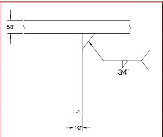
The objective of test 1 was to assess the behavior of a bent that was designed and built using the best ‘current-practice’ of AKDOT. From the typical drawings obtained from AKDOT, it was determined that a fillet weld is the common connection between the pipe column and cap beam for these types of structures. A detail of the weld connection can be seen in Figure 2.24. The size of the fillet weld chosen below was determined by a desire to match the throat thickness with the column wall thickness. A simple check of the weld in bending predicted a failure of the weld prior to developing the full strength of the column section. While increasing the weld size to meet the bending strength of the section was an option, determining the level of performance of the current practice was the goal of test 1. In Table 2.2 a summary of the events that occurred in the test can be seen.

1/2"

3/4"

5/8"

(77)

Table 2.2: Test 1 summary

Ductility Cycle

Load [kips]

Displacement [inches]

Plan view* Notes

µ

2

1

74 6.4

N

South column

Crack appeared to originate at the

bottom of weld

µ

2

-1

59 7.1

N

South column

Crack in heat affected zone below weld and

opened up approx. ¼ “

*Red lines in plan view indicate location, beginning and end of crack

The yield displacement, ∆’y, for this test was 2.49 inches; the equivalent yield

displacement, ∆y, using Equation (2.17) is 3.24 inches. As a result the defined ductility values were µ1 (3.24 in.), µ1.5 (4.86 in.), µ2 (6.48 in), µ3 (9.72 in.), and µ4 (12.96 in.) using

Equation (2.20). In this test, the load controlled cycles showed no damage to the specimen. The same observation was made for the µ1 cycles. During the µ21 cycle, an initial crack was seen in the weld throat. The crack occurred at the bottom of the weld at a load of 74k and displacement of 6.42 inches; seen with in the box A in Figure 2.25. The failure occurred in

(78)

The force-displacement response of test 1 can be seen in Figure 2.27. It should be noted that the cycles in the push and pull direction do not appear to be to the same

displacements, this is because the base moved during the test; the structural displacement is the cap beam displacement minus the base displacement. The force-displacement hysteresis shows the structural displacement. Figure 2.28 shows the base displacement during the test. The base movement yielded slightly different displacements from one cycle to the next. The base displacement was reduced in subsequent tests by removing the rocker bearings beneath the shoes of the pin supports and using an impact wrench to tighten the bolts that hold the shoes in place.

(79)

Figure 2.25: South column, southeast face.

(80)

-150 -100 -50 0 50 100 150

-10 -5 0 5 10

Displacement [inches] F o rc e [ k ip s ]

µ1.5 µ2

µ1

µ-1.5 µ-1

Figure 2.27: Test1 force displacement hysteresis

-10 -5 0 5 10

-2 -1.5 -1 -0.5 0 0.5

Base Movement [inches]

C a p B e a m D is p la c e m e n t [i n c h e s ]

(81)

2.11 Test 2

(82)

2"

1/4"

1/2"

UT 45°

3/4"

Continuous weld for cyclic loading

3/16"

Backer ring min. thickness

5/18"

Figure 2.29: Test 2 connection detail.

Ductility Cycle

Load [kips]

Displacement

[inches] Plan view* Notes

µ

3

1

Loaded past ductility 3to a displacement of 16”, approx. µ5

µ

3

-1

-91 9.72

N

(83)

Table 2.3: Test 2 summary continued

µ

4

1

71 12.96

Buckling on both columns (see

Figure 2.33

µ

4

2

62 12.96

N

South column

Crack at the toe of the weld or a little

below

µ

4

2

62 12.96

N

North Column

Crack lengthen from µ3-1

µ

4

-2 _-58 _12.96

Crack in buckling region of south

column.(see Figure 2.34)

*Red lines in plan view indicate location, beginning and end of crack. Blue lines indicate extent of crack at previous ductility level.

Because of concerns over the construction quality of the specimens, quality control and quality assurance were incorporated into the process. Randy Dempsey, an employee of NCDOT, volunteered conduct the quality assurance. His credentials can be found in

Appendix 6.3. The results for Test 2 quality control can be found in Appendix 6.4

(84)

(9.72 in.), and µ4 (12.96 in.). This specimen experienced significantly less displacement at base. The structural displacement was carefully monitored, and the resulting loading is more symmetrical than test 1. Note that there are minor differences between the displacements for a given ductility level, which are not significant from a performance perspective. The complete force deformation response can be seen in Figure 2.30 and the base displacement can be seen in Figure 2.31. Unfortunately, this specimen was subjected to an accidental ‘overload’ cycle that pushed the specimen to a ductility of 5 when it was intended to be going to ductility 3. From the force displacement response, the maximum load was reached

(85)

-125 -75 -25 25 75 125

-20 -10 0 10 20

µ1µ1.5 µ2

µ3 µ4 µ5 µ-1 µ-1.5 µ-2 µ-3 µ-4

Figure 2.30: Test 2 force displacement hysteresis

-20 -15 -10 -5 0 5 10 15 20

-0.20 0.00 0.20 0.40 0.60 0.80

Base Movement [inches]

C a p B e a m d is p la c e m e n t [i n c h e s ]

(86)

From the start of the test through µ2 no major events occurred. It was decided that a UT inspection during the test could give us more information about what is happening at the connection. The UT inspection was preformed after the µ2 cycles and the load was removed from the specimen for the safety of the technician. As previously noted, between µ2 and µ3 the structure was accidentally loaded to µ5, after which the target load history was continued. Although the first crack was noted at µ3-1, it is possible that the initial damage occurred in the overload cycle to µ5. The crack was noted on the north pile near the neutral axis and can be seen in Figure 2.32. Both columns began to show significant signs of local buckling at the beginning of µ41. A photo of the north column with local buckling near the top can be seen in Figure 2.33. The south column began cracking at base of the local buckling during µ42 as seen in Figure 2.34.

(87)

Figure 2.33: Close up of local buckling on north column

(88)

2.12 Test 3

Test 2 was a significant improvement over test 1, although still not as robust as desired. For test 3, it was desired to determine if the reinforcing fillet played a

complimentary role in its behavior; therefore this specimen had only the full penetration weld. A drawing of the detail can be seen in Figure 2.35. A summary of events can be seen in Table 2.4.

2"

1/4"

1/2"

UT 45°

Continuous weld for cyclic loading

3/16"

Backer ring min. thickness

5/8"

(89)

Ductility Cycle

Load [kips]

Displacement

[inches] Plan view Notes

Over load -100 Unknown

Specimen was loaded past 50%Fy to an unknown load and displacement

µ11 50 3.24

N

North column

µ1.5-2 -61.5 4.86

N

South column

Green arrows show area where

small cracks were seen

µ1.5-2 -61.5 4.86

N

North column

Red line growth of crack and blue

(90)

Table 2.4: Test 3 summary continued

µ2-1 85 12.96

N

North column

Red lines are new crack that

formed

µ2-2 -70 12.96

South Column crack from µ

1.5-2 propagated through weld in

location shown previously

µ23 76

North column crack from µ2-1

propagated through weld in

location shown previously

µ31 -58 9.72

N

South column

New crack on south column shown in red.

(91)

-125 -75 -25 25 75 125

-20 -10 0 10 20

L

o

a

d

[

k

ip

s

]

µ1 µ1.5 µ2

µ3

µ-1

µ-1.5

µ-2

µ-3

(92)

displacement impossible. ∆’y for test 2 was 2.49 inches resulting in ∆y of 3.24 inches. As a result the defined ductility values were µ1 (3.24 in.), µ1.5 (4.86 in.), µ2 (6.48 in), and µ3 (9.72 in.). During the overload a fracture of the weld on the north column occurred at the joint of the weld and the cap beam, as seen in Figure 2.37. The next crack that formed was during µ 1.5-2 on the south column in the northeastern quadrant, as well as some small cracking on the south side of the south column shown in Figure 2.38. The crack in the weld of the north column grew in length and opened during µ 1.5-2 as seen in Figure 2.39. The cracks already formed on both columns continued to grow both in length and width during

(93)

Figure 2.37: North pile first crack along north face arrows on cap beam show extent of crack

Figure 2.38: South column crack on north east after µ1.5-2. The crack is extent of the crack is shown on cap bean with marker

Figure 2.39: South pile crack through weld

Figure 2.40: North column crack propagated through weld

Crack propagation

(94)

Figure 2.41: North Pile after µ31

Figure 2.42: South pile after µ31

2.13 Test 4

With the marginal performance of test unit 3 and the loading error in test 2 (which otherwise performed reasonably well) a repeat of test 2 was selected for test 4. There were two primary questions to be answered: (1) Is the performance of test 2 repeatable, and (2) What, if any, impact did the load history have? A detail of the connection can be seen in Figure 2.29. A summary of the events in test 4 can be seen in Table 2.5. Another difference to note is that Test 4 incorporated the use of sound equipment in order to facilitate the

Cap beam distortion

(95)

detection of cracks and their locations. A series of 10 microphones was employed to monitor acoustic emissions during the test. The goal was to identify the location of any potential damage, and to distinguish between emissions due to pin rotation versus potential damage induced by cracking. The microphone layout is shown in Figure 2.43. With the microphones, it was straightforward to identify emissions due to pin rotation. For example, the

microphones placed at the bottom of each column, as shown in Figure 2.44, registered pin rotations. Even though all microphones registered the pin rotation emissions, those at the bottom measured the highest amplitude.

2 3

4

5

7 8

9

10

North

Figure 2.43: Microphone layout at top of pile

6 1

North

(96)

Ductility Cycle

Load [kips]

Displacement

[inches] Plan view Notes

µ

3

-2 _-90 _-9.91 Local buckling of _{columns near}

weld

µ

3

2 ₆₆ _9.91

N

South column

Crack formed and opened.

Failure of structure.

*Red lines in plan view indicate location, beginning and end of crack.

(97)

-150 -100 -50 0 50 100 150

-20 -10 0 10 20

F

o

rc

e

[

k

ip

s

]

µ1 µ1.5 µ2 µ3

µ-1

µ-1.5

µ-2

µ-3

(98)

Figure 2.47: Crack on south column

(99)

2.14 Summary

In this chapter the experimental program was presented. This presentation consisted of the specimen design and construction, test procedure, instrumentation and an overview of each test. The specimen design was based on actual bridges in Alaska, capacity design principles and the restriction of the CFL lab. The final design was 2 HSS round piles 16” in diameter with a double HP14x89 cap beam whose dimensions and configuration can be seen in Figure 2.4. The construction of the test specimens was accomplished to reproduce field conditions as closely as possible. This process consisted of overhead welding and quality control monitoring throughout the construction sequence. The test procedure for these tests was reverse cyclic loading applied by means of a 220 kip actuator. The test units were pushed and pulled in load control until yield force by increments of quarter yield force. Once the unit has been subjected to the yield force, subsequent cycling was done to reach

(100)

the surface changes of the piles as well. The data from the Optotrack was used to calculate strains, curvature, and local buckling.

Summaries of the four tests were presented in this chapter, highlighting the major events that occurred in each test. For each test the weld detail, summary table, force displacement hysteresis and photos were presented.

Test 1, the current practice in Alaska, was a fillet weld connection between the cap beam and pipe pile. The test unit failed at a ductility of 2 and its failure was in the weld itself. With the poor performance of the current practice, the focus of the study moved to finding an acceptable connection that would conform to design capacity principles such that the inelastic action occurs in the piles and the joint remaining elastic. In order to keep the connection simple as to make it practical and economical, an enhanced welded connection was the focus. With several alternatives considered, a complete joint penetration weld with reinforcing fillet was selected for Test 2. Test unit 2 reach an ultimate ductility of 4, giving it a higher deformation capacity than test unit 1. It is important to note that a loading error occurred during the test from µ2-3 to what should have been µ31. Following the error in loading significant strength degradation occurred with over 20% loss of maximum load occurring at µ33. The failure of the test unit was still in the joint, with significant cracking on both piles at or near the toe of the weld.

(101)

large amount of welding in order to achieve a full penetration weld and a ¾” reinforcing fillet, may have adversely affected the material around the weld known as the heat affected zone. In order to determine if this was the case it was decided to proceed with a test of just the complete joint penetration weld for Test 3. Test unit 3 reached an ultimate displacement ductility of 3. It is important to note that a loading error occurred prior to reaching yield load and may have had an unfavorable effect on the performance of the unit. The failure in Test 3 occurred in the weld itself with significant cracking on both piles.

(102)

CHAPTER III

Analysis of Test Results

CHAPTER 3

3.1 Introduction

The following is a presentation of the analysis of the results from the four tests. The analyses presented in the chapter are the force displacement hysteresis and envelopes, damping, strain profiles, local buckling, and curvature with plastic hinge results.

3.2 Force Displacement Hysteresis

(103)

-150 -100 -50 0 50 100 150

-20 -10 0 10 20

µ1.5 µ2

µ1

µ-1.5 µ-1

Figure 3.1: Test 1 hysteresis

-125 -75 -25 25 75 125

-20 -10 0 10 20

Displacment [inches] F o rc e [ k ip s ]

µ1µ1.5 µ2

µ3 µ4 µ5 µ-1 µ-1.5 µ-2 µ-3 µ-4

-150 -100 -50 0 50 100 150

-20 -10 0 10 20

Displcement [inches] L o a d [ k ip s ]

µ1µ1.5µ2

µ3

µ-1

µ-1.5

µ-2

µ-3

-150 -100 -50 0 50 100 150

-20 -10 0 10 20

µ1µ1.5µ2 µ3

µ-1

µ-1.5

µ-2

µ-3

Table 3.1: Maximum loading information

Test 1 Test 2 Test 3 Test 4

Load

[kips] Ductility

Load

[kips] Ductility

Load

[kips] Ductility

Load

[kips] Ductility Max load 96.50 21 -102.44 3-1 -103.34 overload -100.44 3-1

90% max 86.85 N/A -92.20 3-2 93.01 11 90.40 32

(104)

3.3 Force displacement envelopes.

The force-displacement response envelopes are shown below. These graphs show the peaks on the hysteresis plots from the origin to maximum displacement. Graphs are shown for the first, second, and third cycle envelopes. Clearly, test 2 had the largest drift capacity of all four tests. Comparing the three cycles it is clear that as the cycles progressed the structure showed a decrease in the load carrying ability; most notably in the high levels of ductility. Tests two and four have similar behavior, as expected, since they have the same connection detail.

-150 -100 -50 0 50 100 150

-20 -10 0 10 20

F

o

rc

e

[

k

ip

s

]

-0.14 -0.07 0 0.07 0.14

Drift

Test 1 Test 2 Test 4

(105)

-150 -100 -50 0 50 100 150

-20 -10 0 10 20

F

o

rc

e

[

k

ip

s

]

-0.14 -0.07 0 0.07 0.14

Drift

Test 1

Test 2 Test 4

Figure 3.6: Cycle 2 envelopes

-150 -100 -50 0 50 100 150

-20 -10 0 10 20

F

o

rc

e

[

k

ip

s

]

-0.14 -0.07 0 0.07 0.14

Drift

Test 1

Test 2 Test 4

(106)

3.4 Damping

The hysteretic damping values for each test are presented here. The damping values were calculated using Jacobsen’s approach (Jacobsen, 1930), where the damping is defined as the area contained within one complete cycle of the force displacement response divided by the rigid plastic response that encloses it, shown in Figure 3.8, then multiplied by 2/π.

Displacement

F

o

rc

e

Plastic Response

A_H

Figure 3.8: Graphical representation of damping

(107)

damping for the test units it is necessary to add the elastic viscous damping to the hysteretic damping. A common value for the elastic damping of steel frames are between 2 and 5%, and 2% was selected for the calculations. The elastic damping is based on tangent stiffness and the hysteretic damping is based on secant stiffness. For this reason the elastic damping must be corrected based on nonlinear time-history analysis in order to be combined with the hysteretic damping. The correction factor κ can be seen in Equation (3.2), where λ is equal to -0.617 based upon the Ramberg-Osgood model to represent ductile steel structures (Priestley et al. 2007). The final step is to add the two damping value using Equation (3.3). The results are shown Figure 3.9 where it is evident that there is little difference among the tests. The design equivalent viscous damping for steel frame buildings based upon the Ramberg-Osgood model is included for reference, calculated as a percent using Equation (3.4).

0.4 40 (0.53 0.8)

JAC

hyst

µ

ξ

µ

  

− + 

 

 

 

= +

 

 

(3.1)

λ

κ

=

µ

(3.2)

eq el hyst

ζ =κζ +ζ (3.3)

1 0.05 0.577

eq

µ ξ

µπ  ₋ 

= +  

(108)

0 2 4 6 8 10 12 14 16 18 20

1 1.5 2 2.5 3 3.5 4

Ductility

E

q

u

iv

a

le

n

t

V

is

c

o

u

s

D

a

m

p

in

g

%

Test 2 Test 4 Steel Frame

`

Figure 3.9: Equivalent Viscous Damping

(109)

3.5 Local buckling

The onset of local buckling was of interest to identify. In order to accomplish this identification, pipe pile deformation profiles were created from the Optotrack data. These pile profiles depict an outline of the pile during the test at any given point in time. More information on how the local buckling was identified can be found in section 0on page 38.

3.5.1 Test 1

Using the locations of the LED markers on the North and South face of the South column, plots of the pile profiles are shown in Figure 3.11 and Figure 3.12. Looking at Figure 3.12 it appears that there may be local buckling occurring at the top of the column at

(110)

1 2 3 5 6 7 8 9 10

11 12 13 14 15

16 17

18 19

20

21 22 23 24 25

4 0 5 10 15 20 25

-10 -5 0 5 10

X-axis Y -a x is S o u th F a c e N o rth F a c e

Figure 3.10: Map of LED markers for Test 1

0 5 10 15 20 25