On Genetic Map Functions

(1)

On Genetic

Map

Functions

Hongyu Zhao*

and Terence

P. Speedt

*Department of Biostatistics, University of California, Los Angeles, California 90024 and tDepartment of Statistics,

University of California, Berkeley, Californ.ia 94720

Manuscript received June 12, 1995

Accepted for publication December 20, 1995

ABSTRACT

Various genetic map functions have been proposed to infer the unobservable genetic distance between

two loci from the observable recombination fraction between them. Some map functions were found

to fit data better than others. When there are more than three markers, multilocus recombination

probabilities cannot be uniquely determined by the defining property of map functions, and different methods have been proposed to permit the use of map functions to analyze multilocus data. If for a given map function, there is a probability model for recombination that can give rise to it, then joint recombination probabilities can be deduced from this model. This provides another way to use map

functions in multilocus analysis. In this paper we show that stationary renewal processes give rise to most

of the map functions in the literature. Furthermore, we show that the interevent distributions of these renewal processes can all be approximated quite well by gamma distributions.

G

ENETIC maps consist of different kinds of markers positioned along a chromosome, with their rela- tive locations measured in the map units known as centi- Morgans. During meiosis, crossing over occurs after ho- mologous chromosomes pair and duplicate, resulting in a four-strand structure. Each crossover involves two strands of different origins (nonsister pairs). The genetic map distance in Morgans between a pair of markers on the same chromosome is the average number of crossovers occurring between these markers during meiosis on one chromatid. Because crossovers are not observable, a genetic map function r = M ( d ) is often used to infer genetic distance ( d ) from the observable recombination fraction ( r )

.

In his 1919 paper, HALDANE made three contributions to the study of genetic map functions, as well as defining them. By assuming no crossouer interference (STURTEVANT 1915; MULLER 1916), he derived the map function r = '/*(1 - e-") with inverse d = -

'/'

log(1 - 2 r ) ; he also proposed the empirical inverse map function d = 0 . 7 ~

+

0.3( - '/2 log(1 - 2 r ) ) to account for crossover inter-

ference in the data then available, and he introduced a differential equation method that permitted the con- struction of a variety of map functions.

A commonly used measure of the degree of crossover interference is the coincidence coefficient C involving three markers. Letting

pili*

be the probability of il recombinations in the first interval and

&

recombinations in the second interval, i l ,

4

= 0, 1, Cis defined by

C = P I 1

( P I 0

+

P l l ) (pol

+

Pll).

Corresponding author: Terence P. Speed, Department of Statistics, University of California, Berkeley, CA 94720.

E-mail: [email protected]

Genetics 142: 1369-1977 (April, 1996)

The case of C = 1 corresponds to no crossover interference, while C

<

1 and C

>

1 correspond to positiue and negative crossover interference, respectively. Because the

p,,

can be directly estimated from recombination data in most experimental organisms, C is often used as an empirical index of the degree of crossover interference.

One implicit assumption underlying the use of a genetic map function for one organism is that the func- tional relationship between genetic distances and recombination fractions does not vary across the genome in this organism. This assumption implies that Cshould only depend on the map lengths of the intervals between three markers of interest, say d and h. Noting

{ M ( d )

+

M ( h ) - M ( d

+

h ) ) / 2 , we have

that

p10 +

p11 = M ( 4 ,

pol

+

PI,

= M ( h ) , and

pll

=

Letting h

-,

0, and assuming limbo M ( h ) / h = 1, we obtain the differential equation

" ( d ) = 1 - 2 C ( d ) M ( d ) . (1)

Different choices of C( d ) lead to different map functions, which will be discussed later.

(2)

1370 H. Zhao and T. P. Speed

(GEIRINGER 1944; SCHNELL 1961). The underlying assumption is that the distance between two disjoint intervals is irrelevant to the joint recombination probabilities in these two intervals. However experimental results suggest that the degree of interference varies with the distance between two intervals: the smaller the distance, the stronger the interference. Thus, the above approach is not consistent with experimental results. Nevertheless, this assumption can be and has been used to calculate joint recombination probabilities from map functions. LIBERMAN and KARLIN (1984) proved that a necessary condition to guarantee that the recombination probabilities obtained in this way are nonnegative is that ( -l)kM‘k)(0) 5 0 for all k. They

(inappropriately) termed map functions that always give rise to nonnegative recombination probabilities “multilocus feasible” and showed that many map functions that were found to fit data well did not satisfy these criteria.

If crossovers are viewed as a stochastic point process along the chromatid and a given map function can be realized from a crossover process, multi-locus recombination probabilities compatible with the map function can be obtained by assuming crossovers are generated from this point process. Two classes of point processes have been studied extensively in the literature in the context of modeling crossover interference: renewal processes, reviewed in BAILEY (1961) and MCPEEK and SPEED

(1995), and count-location processes, studied by KARLIN and LIBERMAN (1978) and RISCH and LANGE (1979).

In this paper, we show that for most map functions in the literature there exist stationary renewal processes that give rise to them, and so these map functions are compatible with the analysis of multilocus data via this approach. Moreover, the interevent distributions of the stationary renewal processes corresponding to most map functions can be closely approximated by gamma distributions.

A special class of stationary renewal processes, called chi-square models, which have chi-square interevent distributions with even degrees of freedom, was found to give good fit to data from a variety of organisms (ZHAO et al. 1995b). This class of models, which evolved from an ordinary renewal process model for crossovers on a single meiotic product proposed by FISHER et al. (1947), was mainly studied because of its mathematical tractabil- ity (MCPEEK and SPEED 1995). It was reintroduced by

Foss et al. (1993) from a biological perspective, moti-

vated by observations from experiments on gene conver- sion although there are now serious doubts concerning the appropriateness of this motivation (see FOSS and STAHL 1995). The chi-square model was conveniently denoted as

Cx(

Co) m, which corresponds to a chi-square renewal density with 2(m

+

1) degrees of freedom. US- ing the method of maximum likelihood, chi-square models were fitted to different organisms by ZHAO et aZ.

(1995b). The estimates of m for Drosophila ( m = 4) and

Neurospora ( m = 2) were the same as those obtained by FOSS et al. (1993), who estimated m from the observed ratio of Cx to Co. S. LIN and T. P. SPEED (unpublished results) fitted chi-square models to data on six loci from the CEPH consortium map of human chromosome IO, which was analyzed by WEEKS et al. (1994) using other models, and estimated the parameter m to be 3. Their results suggested the presence of crossover interference during human meiosis. MCPEEK and SPEED (1995) compared the fit of the stationary renewal process model with gamma interevent distributions (the gamma model) with that of other models using one large data set of Drosophila and found that the gamma model gives a better fit than all other models. This fact, together with the observation that for most map functions the interevent distributions for the corresponding stationary renewal processes can be closely approximated by gamma distributions, suggest that to some degree the chi-square model, and more generally, the gamma model, is able to capture the important features of the unobservable crossover process.

After raising the question “What is a genetic map function?”, SPEED (1995) discussed in detail many is- sues related to map functions. It should be pointed out that other methods have also been proposed to extend map functions to handle multilocus data (OWEN 1953;

MORTON and

MACLEAN

1984).

MAP FUNCTIONS AND STATIONARY

RENEWAL PROCESSES

(3)

interference can be distinguished: chiasma interference, where chiasmata on the four-strand bundle do not occur independently of each other, and chromatid interfa- ence, where the choices of nonsister pairs involved in different chiasmata are not independent.

The observation of crossover interference on the meiotic products (single strands) can be the result of chiasma interference alone, the result of chromatid interference alone, or the result of both types of interference. It is interesting to note that the operation of two types of interference can lead to no apparent crossover interference. Consider the case when the chiasma process follows a stationary renewal process with interevent distribution being the gamma distribution with shape parameter and there is complete positive chromatid interference, i.e., the strands involved in one chiasma are never involved in the closest chiasmata to its left and to its right. It is easy to see that the distance between two crossovers on a single meiotic product from this process follows the gamma distribution with shape parameter 1, i.e., the exponential distribution. Therefore crossovers on a single strand appear to occur independently of each other. This example shows that

two types of interference cannot be separated based on single-strand recombination data, where meiotic products from a single meiosis are recovered separately. Therefore tetrad data, where all meiotic products from a single meiosis are recovered together, are often used to detect chromatid interference. Since there is no strong and consistent evidence of chromatid interference (WHITEHOUSE 1982), it is generally assumed that there is no chromatid interference (NCI) in the models proposed in the literature.

The assumption of NCI imposes certain constraints on both recombination and tetrad probabilities (SPEED et al. 1992; ZHAO et al. 1995a). These constraints further impose constraints on map functions (SPEED 1995):

0 5 M ( d ) 5

%,

M ' ( d ) 2 0 ,

M " ( d ) 5 0.

It is also obvious that if the chiasma point process is simple and stationary in the map distance metric, then M ( 0 ) = 0 and " ( 0 ) = 1 (DALEY and VERE-JONES 1988, Section 3.3). We will consider map functions that are defined on a finite interval [O, L] and those defined [O,

00) separately. By imposing one more condition, we say a function M defined on [O, 00) satisfies condition (A) if

M ( 0 ) = 0, (AI)

M ' ( d ) 2 0, for all d, (A2)

Apart from (A5), these conditions are necessary under the assumptions of NCI and that the chiasma process is a simple stationary point process. Condition (A5) postulates that two markers that are very far apart on the same chromosome can be considered very loosely linked, effectively behaving like markers on different chromosomes and segregating independently. More- over, we have the following theorem to characterize this class of map functions. The proof is given in the

Theorem 1: Let Mbe the map function for a stationary

renewal chiasma process satisfymg NCI on a chromosome arm of infinite length. Then M satisfies (A). Conversely, suppose that a function M from [O, 00) into [O, satisfies (A). Then there is a stationary renewal chiasma process whose map function is M and whose renewal density is -M".

For a map function M defined on [O, L] where L

<

00, we say that M satisfies condition (B) if APPENDIX.

M ( 0 ) = 0, (B1)

M ' ( d ) 2 0, for all d , (B2)

" ( 0 ) = 1, (B3)

M " ( d ) 5 0, for all d, (B4)

M ' ( L ) = 0, (B5)

M ( L ) = I/*. (B6)

We say that Msatisfies condition (B)

'

if it satisfies ( B l )

-

(B4) and

M ' ( L )

>

0, (B5)

M ( L )

<

I/*. (B6)'

For map functions defined on [O, L ] , we have the following analogue of Theorem 1 with the proof given in the APPENDIX.

Theorem 2: Let M be the map function for a station-

ary renewal chiasma process satisfying NCI on a chromosome arm of finite length. Then M satisfies (B) or (B)' for any L. Conversely, suppose that a function M from [O, L] into [O, satisfies (B) or (B)'. Then there is a stationary renewal chiasma process whose map function is M and whose renewal density is - M" when d 5 L.

VARIOUS MAP FUNCTIONS

In this section, we apply our two theorems to some map functions in the literature to see if there are stationary renewal processes that can give rise to them.

HALDANE

(1919): MGi(r) = 0.7r

+

0.3(-1/2 log(1 -

2 r ) ) . It is easy to see that " ' ( 0 ) = 0, limr1,2 " ' ( r ) = a, ("I)'

>

0, ( M - ' ) (0) = 1, lim,.+1,2 ("I) = 03, and ( M " l ) r r z 0. So M , satisfies condition (A), and there is a stationary renewal process giving rise to MHz.

(4)

1372 H. Zhao and T. P. Speed

1.5 -

1.0 -

.- b

z

s

0.5 -

0.0 -

0.0 0.5 1

.o

1.5 2.0

Genetic Distance (Morgan)

FIGURE 1.-Comparison between the interevent density

( - M k ) of the stationary renewal process corresponding to

the Kosambi map function and two gamma densities:

gamma(4,2) and gamma(2u,u), where u is 1/(2 log(2) - 1)

=

2.6.

the interval [O, 1 / 4 ~ ] , and it is easy to check condition (B) in this case, with I , = '/47r. Thus there is a stationary renewal process having it as a map function, although the chromosome arm is rather short.

KOSAMBI (1944): MK( d ) = tanh ( 2 d ) . Since

nil,(

d )

e - 2 d ) S , it is easy to check that (A) is satisfied. The interevent distribution for the corresponding stationary renewal process is 16(e2d - e - 2 d ) / ( e 2 d

+

e?)'. KOSAMBI

(1944) found that this map function gave good fit to Drosophila data. FISHER et al. (1947) noticed that the Kosambi map function is very close to the map function from a renewal process with interevent distribution being chi-square with four degrees of freedom. Both - M ' i and the density of gamma(4,2) are plotted in Figure 1. The density of a gamma(b,g) variable is [ b ( b ~ ) ~ ' e - " ] / T ( g ) . The mean and variance of -M'k are and log(2)

/2

-

'/+

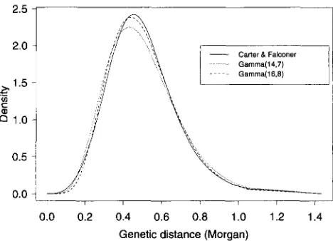
The density of gamma(2u, u ) , where u = 1/(2 log(2) - l ) , which has the same mean and variance as -M';c, is also plotted in Figure 1. CARTER and FALCONER (1951):

K;,(T-)

= 1/4(tan"(2r)

+

tanh-'

(27)).

Here McF( d ) is the solution of the differential equation M ' ( d ) = 1 - 16M4(d). This map function

was found to fit mouse data better than other map functions (CARTER and FALCONER 1951). Since M'&(d) = -64M&;( d ) (1 - 16M&( d ) )

,

and M,, 5 (A) is satis-

fied. The corresponding stationary renewal process has interevent distribution 64M;?.,(d) (1 - 16M&(d)). The Carter and Falconer map function -M'&(d) together with the density of gamma(14,7) and gamma(l6,S) are plotted in Figure 2. It was found that Cx( C O ) ~ and Cx( C O ) ~ give the best fit for two mouse data sets in BLANK et al.

(1988) and TODD et al. (1991) (ZHAO 1995); the choice of the Carter and Falconer map function would be equiv- alent to using the

CX(CO)~

model.

STURT (1976): M s ( d ) = 1/2(1 - (1 - $',)e

1,

0 5 d 5 L. This map function arises via a count-location

= 4(2"

+

e-2d)-2, and M ' k ( d ) = -16(e2fi - e - 2 d ) / ( e 2 d

+

- d ( Z L - I ) / I ,

2.5

2.0

2. 1.5

6

1.0

.-

v)

C

0.5

0.0

0.0 0.2 0.4 0.6 0.8 1.0 1.2 1.4

Genetic distance (Morgan)

FIGURE 2.-Comparison between the interevent density

(-Mcl.) of the stationary renewal process corresponding to the Carter and Falconer map function and two gamma densi-

ties: gamma( 14,7) and gamma(16,8).

chiasma process that begins with an obligatory crossover event on the arm, followed by a Poissondistributed number of crossover events having mean 2L - 1. The total genetic length is thus L. This map function fails (B5) but satisfies (B6), and so no stationary renewal process can give rise to it.

+

w & M F $ ( ~ T )

+

w.&lk1(27), where wH =

p

(1 - 2 p ) ( l

p )

(1 - 2p)/3, WM (1 -

p ) ( l

- 2 p ) ( l - 4p), and

M i ' , M i ' , M;:, and M&' are the inverse of the Haldane, Kosambi, Carter-Falconer, and Morgan map functions. It is easy to check that for any

p,

wH, wK, w , ~ , and whf cannot all be positive. Indeed MR does not satisfy our necessary conditions (WEEKS 1994). Following RAO et

al.'s idea, we might try to define a map function from a set of n

>

2 map functions by letting " ' ( 7 ) =

wt(p)

MY1(r), where

wL(p)

is a polynomial in

p

of order n - 1, and M ( d ) reduces to

Mi(

d ) when

p

=

p ,

for given 0

< pl

< p, <

-

*

p,

<

1. But it can be shown that for no

p

can the

w,(p),

i = 1, 2,

. . .

, n,

so defined all be positive. Therefore this approach to obtaining empirical map functions from existing map functions would seem questionable.

m o

(1977): Mi1(?") = wHkfb'(27)

+

WKMK'(27)

- 4p)/3, WK = -4p( 1 -

p )

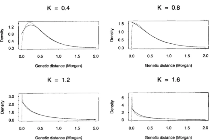
( 1 - 4p), wcp = 32p( 1 -

FEUENSTEIN (1979): M,( d ) = ' / n (1 - +?2(K"L)ri)

/

(1 -

( K - l ) e 2 ( K - 2 ) d ) . When K

>

2, lim&m & ( d ) = ( K -

1) f and so no stationary renewal process exists with this mapping function. Because Mk-(d) = ( K -

2)2e2("d/(1 - ( K - l ) e 2 ( K - 2 ) " ) 2 , M,(d) = 2 ( K -

2)5e2(K-Z)d (1

+

( K - l)e2(K-2)" ) / ( I - ( K - l ) e Z ( w d 3

1.

>

(5)

K

=

0.4 K

=

0.8

0

0”

0.4

0.0

1.2 ._

E 0.8

0.0 0.5 1.0 1.5 2.0 Genetic distance (Morgan)

K

= 1.2

0.0 0.5 1.0 1.5 2.0

1.5

p

1.0

0”

0.5 0.0

0.0 0.5 1.0 1.5 2.0 Genetic distance (Morgan)

K

=

1.6

0.0 0.5 1 .o 1.5 2.0

FIGURE 3.-Comparison between the interevent density ( - M i , solid curve) of the stationary renewal process corresponding

to the Felsenstein map function and the gamma density (dotted curve) having the same mean and variance for K = 0.4, 0.8, 1.2, and 1.6.

close agreement between Felsenstein’s family and the gamma family.

KARLIN and LBI- (1978, 1979): Mcl,(d) = [1 - c(1 - d / L ) ] . This class of map functions arise from the count-location process, where c(s) = x k z o C k S k is a

probability generating function of a count variable c

with distribution ( c k ) , and d(1) = 2L. McL is only well defined for finite L, It is easy to check that ( B l )

-

(B4) are satisfied. Because M,,.(L) = 1/2 (1

-

cg) and M ,

( L ) = c1/2L, from Theorem 2, there is a corresponding stationary renewal process for Mc12 only if (1) ~0 = 0 and q = 0, or (2) re

>

0 and el

>

0.

DISCUSSION

In constructing genetic maps, map functions have been used to infer the unobservable genetic distance between two markers from the observable recombination fraction between these markers. Different genetic map functions embody different degrees of crossover interference among the crossovers. It has been observed that different organisms have different degrees of crossover interference, it so is not surprising that different map functions have been found suitable for different organisms. The major disadvantage of using map functions is that joint recombination probabilities cannot be uniquely determined in terms of them when there are more than three markers. Various approaches have been proposed to extend map functions to handle multilocus data.

One widely adopted approach, which was suggested

by GEIRINGER (1944) and SC:HNEI.L (1961) and thor-

oughly studied by LIRERMAN and KARLJN (1984), em-

bodies the assumption that for a pair of noncontiguous intervals, the probabilities for joint recombination pat- terns across these intervals do not depend on the distance between these two intervals, something that is not consistent with observations. Those map functions that can be extended to multilocus data through this a p proach have been (inappropriately) called “multilocus feasible” (LIBERMAN and KARLIN 1984). This criterion excludes many functions that were found to fit well to recombination data, such as the Kosambi map function.

In this paper, another approach is proposed to extend map functions for the analysis of multilocus data. If for any given map function, we can find a point process model that gives rise to this map function, then multilocus joint recombination probabilities can be obtained in a way that is completely compatible with the map function. Stationary renewal processes can give rise to many map functions. From this perspective, most map functions that are not multilocus feasible ac- cording to KARLIN and LIBERMAN can in fact be extended to permit the analysis of multilocus data.

Another measure of interference, called S4 by Foss et al. (1993), is formally defined as

S4( d ) = lim lim

PI

1

k.0 k.0 ($10

+

P I 1

1

( P O I

+

p 1 J

where the

pi,a2

are as in the definition of C, with one interval having map length h, the other interval map length k, and the two intervals being separated by a map distance d. It seems that S, captures more important aspects of crossover interference than does C

(6)

1374

n = l

H. Zhao and T. P. Speed

n = 3

2.0

n

0.0 0.5 1.0 1.5 2.0 2.5 3.0 Genetic distance (Morgan)

n = 5

3.0 2.5

2.0

2 1.5

._

0"

1.0

0.5 0.0

0.2 0.4 0.6 0.8 1.0

Genetic distance (Morgan)

0.2 0.4 0.6 0.8 1.0 1.2 1.4

n = 6

0.0 0.2 0.4 0.6 0.8

FIGURE 4.-The interevent density of the stationary renewal process corresponding to the map function M that satisfies M' =

1 - (2M)"for n = 1, 3, 5, 6.

mined from a map function, it can be calculated given a particular way of generalizing map functions to multilocus data and compared to empirical estimates. For the count-location processes, S, is constant for all d, whereas S4 has various forms for the stationary renewal processes. The values of S4 as a function of d were estimated from a large Drosophila data set and were very close to the S4 values under the chi-square model (Foss et al. 1993, MCPEEK and SPEED 1995).

Map functions cannot and should not be expected to reflect chiasma or crossover interference in anything but the most superficial way. Indeed, a map function could arise from both the stationary renewal process and the count-location process, although the interference differs greatly between these two classes of models. For example, the map function M ( d ) = d/ (1

+

2 d ) could arise from a stationary renewal process with interevent distribution 4(1

+

2 d ) - ' , and it could also arise from a count-location model with ck = ' / 2 k , where iz

2 0 (LIBERMAN and KARLIN 1984). Under the count- location model, the length of the chromosome defined by c = ( c k ) is so M ( d ) is only defined on

[o,

1/2], while d can range from 0 to 00 for the stationary renewal

process model.

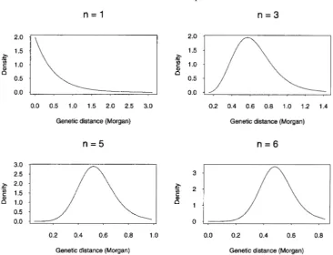
Note that for the stationary renewal processes corresponding to most map functions discussed, the interevent distributions can often be well approximated by gamma distributions. Recall that the Haldane, Kosambi, and Carter and Falconer map functions are all solutions to the differential Equation 1 with C ( d ) = (2M)"". It can be shown that map functions M obtained via this

approach always satisfy (A). Figure 4 displays plots of

(7)

interference is generally considered valid. The use of map functions and stationary renewal processes requires that the degree of interference be the same across the chromosome, which is an obvious simplifica- tion. But a large amount of data will probably be necessary to permit the detection of nonstationarity of the underlying process.

In summary, we have shown that for most genetic map functions, there is a corresponding stationary renewal process, and that these map functions can be extended to permit the analysis of multilocus data by calculating joint recombination probabilities from their corresponding renewal processes. This provides another way of generalizing a given map function to the multilocus situation, although it seems unlikely that there are efficient methods to estimate genetic distances and other parameters from multilocus recombination data under completely general renewal processes. The calculation of multilocus recombination probabilities for stationary renewal chiasma processes is discussed in the APPENDIX. However, comparisons between the interevent distribution of general stationary renewal processes and that of chi-square distributions suggest that this class of renewal processes provides sat- isfactory approximations to the renewal processes corresponding to most genetic map functions in the literature. With the limited amounts of data currently available, it will probably be hard to distinguish these models, although we can look forward to many refine- ments in the future.

This work was supported by National Institutes of Health grant H G 0109341. The authors thank two referees for their helpful comments.

LITERATURE CITED

BAILEY, N. T. J., 1961 Introduction to the Mathematical Theory of Genetic Linkage. Oxford University Press, London.

BLANK, R. D., G. R. CAMPBELL, A. CALABRO and P. D. EUSTACHIO, 1988 A linkage map of mouse chromosome 12: localization of

Igh and effects of sex and interference on recombination. Genet- ics 120: 1073-1083.

CARTER, T. C., and D. S. FALCONER, 1951 Stocks for detecting linkage in the mouse and the theory of their design. J. Genet. 50:

CARTER, T. C., and A. ROBERTSON, A,, 1952 A mathematical treat-

Proc. Roy. SOC. B 139: 410-426.

ment of genetical recombination using a four-strand model. COBBS, G., 1978 Renewal process approach to the theory of ge-

netic linkage: case of no chromatid interference. Genetics 89:

DALEY, D. J., and D. VERE-JONES, 1988 A n Introduction to the Theory of Point Processes. Springer-Verlag, New York.

FELLER, W., 1971 An Introduction to Probability Theory and Its Applica- tions. Vol. 2, Ed. 2. John Wiley, New York.

FELSENSTEIN, J., 1979 A mathematically tractable family of genetic mapping functions with differents amount of interference. Ge- netics 91: 769-775.

FISHER, R. A,, 1947 The theory of linkage in polysomic inheritance. Phil. Trans. Roy. SOC. B. 233: 55-87.

FISHER, R. A., M. F. LYON and A. R. G. OWN, 1947 The sex chromosome in the house mouse. Heredity 1: 335-365,

FOSS, E., and F. W. STAHL, 1995 A test of a counting model for chiasma interference. Genetics 139: 1201-1209.

FOSS, E., R. WDE, F. W. STAHLand C. M. STEINBERG, 1993 Chiasma 307-323.

563-581.

interference as a function of genetic distance. Genetics 133:

GEIRINGER, H., 1944 On the probability theory of linkage in Mende- lian heredity. Ann. Math. Statist. 15: 25-57.

HALDANE, J. B. S., 1919 The combination of linkage values, and the calculation of distances between the loci of linked factors. J.

Genetics 8: 299-309.

JENNINCS, H. S., 1923 The numerical relations in the crossing over of the genes with a critical examination of the theory that the genes are arranged in a linear series. Genetics 8: 393-457. KARLIN, S., and U. LIBERMAN, 1978 Classification and comparisons

of multilocus recombination distributions. Proc. Natl. Acad. Sci.

KARLIY, S., and U. LIBERMAN, 1979 A natural class of multilocus recombination processes and related measure of crossover interference. Adv. Appl. Prob. 11: 479-501.

KOSAMBI, D. D., 1944 The estimation of the map distance from recombination values. Ann. Eugen. 12: 172-175.

LIBERMAN, U., and S. KARLIN, 1984 Theoretical models of genetic map functions. Theor. Pop. Bio. 25: 331-346.

LUDWIG, W., 1934 Uber numerische beziehungen der crossover- werte untereinander. Z. indukt. Abatamm. Vereb. 67: 58-95. MATHER, K., 1935 Reductional and equational separation of the

chromosomes in bivalents and multivalents. J. Genet. 30: 53-78. MATHER, K , 1936 The determination of position in crossing over.

J. Genet. 33: 207-235.

MATHER, K, 1937 The determination of position in crossing over. 11. The chromosome lengthchiasma frequency relation. Cytologia, Jub. Vol., 514-526.

MCPEEK, M. S., and T. P. SPEED, 1995 Modeling interference in genetic recombination. Genetics 139: 1031-1044.

MORGAN, T. H., and C. B. BRIDGES, 1916 Sex-linked inheritance in Drosophila. Carniegie Institute of Washington.

MORTON, N. E., and C. J. MACLEAN, 1984 Multilocus recombination frequencies. Genet. Res. 44: 99-108.

MUILER, H. J., 1916 The mechanism of crossing over. Am. Nat. 50:

OWEN, A. R. G., 1953 The analysis of multiple linkage data. Heredity

RAO, D. C., N. E. MORTON, J. LINDSTEN, M. HULTEN, and S. YEE, 1977 A mapping function for man. Hum. Hered. 27: 99-104. RISCH, N., and K LANGE, 1979 An alternative model of recombina-

tion and interference. Ann. Hum. Genet. 43: 61-70.

SCHNELL, F. W., 1961 Some general formulations of linkage effects in inbreeding. Genetics 46: 947-957.

SPEED, T. P., 1995 What is a genetic map function? in Genetic M a p ping and DNA Sequencing, edited by T. P. SPEED and M. S. WATER-

MAN. Springer-Verlag, New York.

SPEED, T. P., M. S. MCPEEK and S. N. EVANS, 1992 Robustness of the no-interference model for ordering genetic markers. Proc. Natl. Acad. Sci. USA 89: 3103-3106.

STAM, P., 1970 Interference in genetic crossing over and chromosome mapping. Genetics 92: 573-594.

STURT, E., 19783 A mapping function for human chromosomes. Ann. Hum. Genet. 4 0 147-163.

STURTEVANT, A . H., 1915 The behavior of chromosomes as studied through linkage. Z. lndukt. Abstammungs. Vererbugsl. 13:

TODD, J. A., T. J. AITMAN, R. J. CORNALL, S . GHOSH, J. R. HALL el al., 1991 Gr netic analysis of autoimmune type 1 diabetes mellitus in mice. Nature 351: 542-547.

WEEKS, D. E., 1994 Invalidity of the Rao map function for three loci. Hunt. Hered. 4 4 178-180.

WEEKS, D. E.,

1s.

M. LATHROP and J. Om, 1993 Multipoint mapping under ge letic interference. Hum. Hered. 43: 86-97.

WHITEHOUSE, H. L. K , 1982 Genetic Recombination: Understanding the Mechanism. John Wiley, New York.

ZHAO, H., 1995 StatisticalAnalysis of Genetical Interfmence. PhD thesis, University of California a t Berkeley, Berkeley.

Z ~ O , H., M. S., MCPEEK and T. P. SPEED, 1995a Statistical analysis of chromatid interference. Genetics 139: 1057-1065.

ZHAO, H., T. 1’. SPEED and M. S. MCPEEK, 1995b Statistical analysis of crossover interference using the chi-square model. Genetics

139: 1045-1056. 681-691.

USA 75: 6332-6336.

193-221, 284-305, 350-366, 421-434.

7: 247-264.

234-287.

(8)

1376 H. Zhao and T. P. Speed

APPENDIX

Proof of Theorem 1: Suppose the crossovers are

from a stationary renewal chiasma process with interevent density J: Without loss of generality, we may as- sume the mean interevent distance is p = 1/2, so the metric is simply genetic distance. For any point .;3f1, say, on the chromosome, the chance that the first crossover after .?Il occurs in the small interval (y,y

+

dy) is

The probability of no crossovers occurring before .?I2, which is map distance d from is

Po

= Jdrn

( 2

[ f ( t ) d t } d Y .

Using Mather's formula (MATHER 1935), which asserts that the recombination fraction r between any two markers is

where

Po

is the probability of zero crossovers occurring between these markers, we have

M ( d ) = r = 2

{

1 -

2

Jdm

[

f ( t ) d t d y } .

It is easy to verify that M so defined satisfies (A). Conversely, if M satisfies (A), then

Iom

( - M " ( t ) ) d t =

M ( 0 )

= 1.

Thus -M" is a probability density function on [0, m)

.

If the interevent distribution in a stationary renewal process is -MIr, then their mean is

[r

( - t M ' ( t ) ) d t = JOE

[

( - M " ( y ) ) d y d t

= Jorn M ' ( t ) d t =

Thus, the map function generated from the stationary renewal chiasma process with interevent distribution

-M" is

1

(1 - 2

p

Jm

( - M " ( t ) d t ) d y ) = M ( d ) .

2 d y

Proof of Theorem 2: Note that

and (B6)' are true. The first part of this theorem can then be proved as in Theorem 1.

If M ( L )

<

and M ' ( L )

>

0, we may define an extended map function M,(d) on [0, 00) as follows:

( M ( d ) if d

<

I,

where a = - M ( L ) and

a0

= M ' ( L ) . It can be verified that M E ( d ) so defined satisfies (A) in Theorem

1. So there is a stationary renewal process whose corre-

sponding map function is M f i ( d )

,

which coincides with

M ( d ) on [0, L ] . If M ( L ) = and M ' ( L ) = 0, it can be easily shown that the stationary renewal process with renewal density -MIr gives rise to M.

Calculating rnultilocus recombination probabilities for

stationary renewal chiasma processes: Suppose that

Yo,

Y,

,

. . .

, 'I(, are n

+

1 consecutive loci along a chromosome, defining n genomic intervals I, = [ -?lo, . . V I ),

. . .

,

Z

,

= [ . 3 n - l , . Y n ) of map lengths d l , d2,

. . .

, d,,, respectively. Extending the notation introduced earlier, we denote by

pfl,,

,4, the joint recombination probability of having zl = 0 or 1 recombination across interval

4 ,

j = 1,

. . .

, n. The question we address here is the calculation of all such probabilities p =

(pi,,

, .+,) when the underlying chiasmata form a renewal process stationary in the genetic distance metric and NCI is assumed. To do so we make use of the so-called linkag values, denoted by z =

( . z j , . ,

J ,

where z~,, , ,~~ is the probability of finding no chias mata in the union

U{4$

= l} of those intervals for which

2; = 1, see SPEED et al. (1992) for fuller details. We also make use of some well known facts from renewal theory and refer to FELLER (1971) for derivations. Suppose that we have a stationary renewal process with interevent density f and mean interval length p. The distance of an arbi- trary but fixed point on the chromosome to the next chiasma to its left (respectively right) is called the backward (respectively forward) recurrence length (tradition- ally called "time"), and if these are denoted by ,8 and

4,

then

where F is the cumulative distribution function (c.d.J )

corresponding to J:

Now let us consider the calculation of the linkage values z = (G,, , .J. For n = 2 this is quite straightfor- ward. Suppose that we want to calculate zIo, the probability of no crossovers in Zl. We regard 71, as the arbi- trary but fixed point in the preceding discussion, and put u = d l and u = 0 in (2), obtaining the formula zl,, = 1 - F*(dl ), where F* is the c.d.5 corresponding to

f*

= p" (1 - F ) . Similarly, = 1 - F * ( d 2 ) , zI 1 = 1 - F*(dl

+

d 2 ) , and zoo = 1. All of these expressions are

easily computed as long as Fy: is tractable.

(9)

Map Functions

z = ( A quick run through all eight possibilities re- veals that all but zlol can be obtained in the manner just illustrated with n =

2.

For example, zloo = 1 - P ( d 1 ),

roll = 1 -

P ( 4

+

4 ) ,

etc. It turns out that the calculation of zlol, in general requires summing a series of multiple integrals, and that the only known cases in which these integrals simp19 into something tractable are variants on thinned Poisson processes. Let us see why.

First we recall that zlol is the probability of no chiasmata in either 1, or 13; there may be zero, one or more in 12, where the count is not constrained. Thus an initial reduction of zlol is as follows:

m

ZlOl = 2111

+

< k ,

k= 1

where zlll is the probability of no chiasmata in Il U I2

U I3 ( = 1 - F* ( dl

+

4 +

& ) ), and

ck

is the probability of k chiasmata in

I2

and none in Il or Is. We now give an expression for <k that, in general, does not simplify,

and we remark that we know of no substantially simpler alternative expressions in the literature on renewal processes.

If there are to be k 2 1 chiasmata in I,, we may

denote the forward recurrence interval length from X I

to the first event by

yl

, and the k subsequent interevent distances by

p,

y3,

. . .

,

y k , y k + l . Further we may denote

by

yo

the backward recurrence distance to the first event to the left of .Wl. With this notation we can readily check that the probability ( k is the ( k

+

2)-fold integral

of the joint density of

( y o , y l ,

. . .

,

y k , y k + l ) over the range

y k + l

>

4 +

&}.

The joint density of yo,

.

. .

,

y k + l is the

product

{ Y O

>

dl1

n

{ y l

+

'

+

y k

<

41

{ y l

+

'

+

y k

+

P"f*(YO

+

J l )

x

n;:;

f ( Y J >

and so our assertion is demonstrated: zlol is an infinite sum of multiple integrals and will have a tractable expression only when these sums and integrals simplify. For each n 2 3 there is one or more G,. , .2, requiring such expressions, and so far it is only the class of chi- square renewal processes (ZHAO et d . 199513) and a