Copyright1998 by the Genetics Society of America
Assessing the Impact of Secondary Structure
and Solvent Accessibility on Protein Evolution
Nick Goldman,* Jeffrey L. Thorne
†and David T. Jones
‡*Department of Genetics, University of Cambridge, Cambridge CB2 3EH, United Kingdom,†Program in Statistical Genetics, Department of Statistics, North Carolina State University, Raleigh, North Carolina 27695-8203 and
‡Department of Biological Sciences, University of Warwick, Coventry CV4 7AL, United Kingdom
Manuscript received October 5, 1997 Accepted for publication February 17, 1998
ABSTRACT
Empirically derived models of amino acid replacement are employed to study the association between various physical features of proteins and evolution. The strengths of these associations are statistically evaluated by applying the models of protein evolution to 11 diverse sets of protein sequences. Parametric bootstrap tests indicate that the solvent accessibility status of a site has a particularly strong association with the process of amino acid replacement that it experiences. Significant association between secondary structure environment and the amino acid replacement process is also observed. Careful description of the length distribution of secondary structure elements and of the organization of secondary structure and solvent accessibility along a protein did not always significantly improve the fit of the evolutionary models to the data sets that were analyzed. As indicated by the strength of the association of both solvent accessibility and secondary structure with amino acid replacement, the process of protein evolution—both above and below the species level—will not be well understood until the physical constraints that affect protein evolution are identified and characterized.
W
IDELY used models of sequence evolution pro- ofKimura (1983). In macroevolutionary applications, theJukes-Cantor(1969) model may often be sufficient vide notoriously poor fits to actual sequence data(e.g., Goldman 1993;Goldman andYang 1994). For for accurate reconstruction of phylogenies.
Nevertheless, the limitations of widely used models example, the infinite sites model of population genetics
assumes that distinct mutational events never affect the of sequence evolution often prevent more refined and informative questions from being addressed. A key to same site in a DNA sequence. This assumption cannot
modelling and understanding the evolutionary process be reconciled with the data: this model predicts that at
is identification and characterization of the constraints most two nucleotide types will be represented in a
col-that evolution “perceives” as proteins diverge. Selective umn of a sequence alignment, yet it is often the case
constraints on protein structure would be expected to that an actual aligned data set contains one or more
give rise to associations between patterns of amino acid alignment columns where three or sometimes all four
replacement and structure. In this article, we extend our nucleotide types are represented. For these data sets,
earlier approach (Thorneet al. 1996) for characterizing the infinite sites model can be rejected by inspection.
these associations by increasing the number of second-More sophisticated models (e.g., Jukes and Cantor
ary structures distinguished by the evolutionary model 1969; Hasegawaet al. 1985;Yang 1994) are typically
and by considering solvent accessibility (i.e., whether or employed when sequences from different species are
not a residue is near the surface of a protein and rela-being compared. These may be superior to the infinite
tively exposed to solvent). We also add a more realistic sites model in that they cannot be rejected by inspection,
description of secondary structure organization along but these also tend to be rejected by goodness-of-fit tests
a protein sequence. such as the one proposed by Goldman(1993).
There is a tradition of studies (e.g.,Overingtonet al. Although their assumptions may be violated and there
1990;Lu¨ thyet al. 1991;Tophamet al. 1993;Wakoand may be statistical grounds for rejecting them, simple
Blundell1994) that attempts to associate amino acid models of sequence evolution may still be adequate
replacement patterns and protein secondary structure for investigating the questions to which they are often
or solvent accessibility, but these studies were performed applied. In population genetics, the infinite sites model
without direct consideration of evolution and their may be good enough for testing the neutral hypothesis
findings are therefore difficult to apply to evolutionary questions. The work ofKoshi andGoldstein(1995) is more interpretable from an evolutionary perspective
Corresponding author: Nick Goldman, Department of Genetics,
Uni-but was not aimed at the study of evolution and instead
versity of Cambridge, Downing Street, Cambridge CB2 3EH, UK.
E-mail: [email protected] addressed prediction of secondary structure and solvent
Figure1.—Observed and predicted secondary structure length distributions. Open bars are empirically observed frequencies
of secondary structure lengths. Solid bars are predicted frequencies. The predicted frequencies for Figures 1 (A–D) assume a geometric length distribution. The predicted frequencies for Figures 1 (E–G) are those used by the HMM. For coils, the HMM uses the geometric distribution depicted in (D). (A) Observed and geometric distributions of helix lengths (n51339). (B) Observed and geometric distributions of sheet lengths (n51862). (C) Observed and geometric distributions of turn lengths (n54482). (D) Observed and geometric distributions of coil lengths (n55113). (E) Observed and HMM distributions of helix lengths (n51339). (F) Observed and HMM distributions of sheet lengths (n51862). (G) Observed and HMM distributions of turn lengths (n54482).
accessibility. Other recently proposed models incorpo- and coil. For each secondary structure type, we further divide sites into those that are relatively exposed to rate variation of preferred amino acid residues among
sites (e.g.,Brownet al. 1993;Bruno1996) but are not solvent and those that are buried.
Having two accessibility classes, buried (b) and ex-designed to facilitate study of the relationship between
protein structure and evolution. With the approaches posed (e), for each of the four secondary structure types (H, E, T, C) gives rise to a model with protein sites that described here, associations between protein secondary
structure, solvent accessibility, and the pattern of pro- belong to one of eight categories (Hb, He, Eb, Ee, Tb, Te, Cb, Ce). We use a hidden Markov model (HMM) tein evolution can be investigated from within a
likeli-hood inference framework. approach (seeChurchill1989;Asaiet al. 1993;White
et al. 1994; Yang 1995; Felsenstein andChurchill
We assume that each site in a protein belongs to one
of several categories. The categories need to be prede- 1996) to describe organization of these eight categories along a protein sequence, and we describe the length termined, but the category to which each site belongs
namic programming-based similarity search (Gotoh1982) to
these changes is both relatively complicated and
com-find sequences of.30% identity with the sequence of known paratively realistic when contrasted with previous
ex-structure. Each family found in this manner is aligned via the plicit models of protein sequence evolution. In the sec- multiple sequence alignment method ofTaylor(1988).
tions that follow, we first describe the model. We then Secondary structure assignments and solvent accessibility scores are calculated for the protein of known structure with investigate several data sets to understand how much
the DSSP program (KabschandSander1983) and are
extrap-various features of the model improve its fit.
olated across each aligned sequence family by assuming that all residues in an alignment column share the secondary struc-ture and solvent accessibility classification of the homologous MATERIALS AND METHODS
residue in the protein with experimentally determined ture. Residues inserted into the middle of a secondary struc-BRKALN database:Fixed parameters of the model were
estimated as described below from a database of structure- ture element are assigned that secondary structure, and inser-tions elsewhere are defined as having unknown secondary related amino acid sequence alignments. The BRKALN
data-base maintained by D.T. Jones (unpublished results) contains structure. Using the January 1995 release of PDB and release 25.0 of OWL resulted in the BRKALN database containing amino acid sequences classified into families of closely related
sequences for which the tertiary structure of at least one mem- 207 families of sequences.
The DSSP assignments that occur in the BRKALN database ber has been experimentally determined. The database is built
by extracting nonhomologous sequences from the Brookha- are classified as follows: H, helix; E, sheet; S and T, turn; all others (i.e., B, “.”, G, and I), coil. The decision to classify S ven Protein Databank (PDB;Bernsteinet al. 1977). Low
reso-lution (.2.6A˚ ) and NMR structures are excluded. Each se- and T as a separate turn category instead of as coil (as in
Thorneet al. 1996) was made because the DSSP assignments
quence is compared to the OWL nonredundant protein
Figure 2.—Examples of permitted transitions among the 38 HMM states. Arrows indicate the permitted transitions among
the states illustrated and are labelled with the parameter combinations that define the transition probabilitiesrij. Thicknesses
of arrows are approximately proportional to the values of the correspondingrij. (A) Twelve sheet states. (B) Four turn states.
(C) Two coil states. (D) All permitted transitions from the Eb3state. The HMM may progress to either of the next sheet states
and rates that are qualitatively similar to one another. DSSP can leave the sheet. This arrangement of 12 sheet states is illustrated in Figure 2A. The manner of controlling the distri-solvent accessibility values were converted to two states, buried
(accessibility,10%) and exposed (accessibility$10%). Rela- butions of secondary structure lengths is described below. The choice of six position-specific sheet states each for bur-tive accessibility was estimated by using a fully extended
Gly-X-Gly tripeptide as the reference state. This resulted in approx- ied and exposed was made with a likelihood ratio testing procedure that took into account the number of parameters imately half of the sites in known structures of the BRKALN
database being classified as buried and half as exposed. There being estimated and the improvement in goodness-of-fit as the number of position-specific states increased. We use nEto
is scope for more refined solvent accessibility schemes to be
explored in the future. represent the number of position-specific states for each of buried and exposed sheet. Similar considerations suggested Replacement processes: Each combination of secondary
structure and accessibility status is associated with a particular that the helix states Hb and He each be expanded into nH5
10 states (Hb1, Hb2,..., Hb10and He1, He2,..., He10) and that the
amino acid replacement process. As is the case for most widely
used models of nucleotide substitution and amino acid re- turn states Tb and Te be expanded to Tb1, Tb2, Te1, and Te2
(nT52). Only two coil states (denoted Cb1and Ce1) are in
placement, our models of amino acid replacement are
Marko-vian with respect to time. To specify the process of evolution the HMM (nC 5 1) because coil represents a collection of
diverse minor secondary structure elements (including but for a specific replacement category k that is one of the eight
in our model, there are parameters ak
ij, the relative rate of not limited to loops) that together have approximately a
geo-metric length distribution. In summary, this led to 38 hidden change from type i to j. Slight modifications (Joneset al. 1992;
Goldmanet al. 1996;Thorneet al. 1996) of the approach by states comprising 10 buried and 10 exposed helix states, six
buried and six exposed sheet states, two buried and two
ex-Dayhoffet al. (1972, 1978) are used to base estimates ofakij
on observed amino acid replacement counts. These counts posed turn states, and one buried and one exposed coil state. The model requires that all sites with a particular secondary are made by comparing pairs of sequences in the BRKALN
database that are 85% or more identical and by recording the structure and accessibility status experience the same amino acid replacement process, regardless of relative position within number of times for replacement category k that amino acid
type i is observed in one sequence of the pair and type j is their secondary structure element. For example, a buried site that begins a helix (Hb1) and a buried site in the third position
observed at the corresponding site in the other.
Hidden Markov model:Neither the secondary structure nor of a helix (Hb3) share the same replacement process. Thus,
each of the 38 HMM states corresponds to a particular one the solvent accessibility at one site in a protein is independent
of that at nearby sites. In fact, secondary structures at adjacent of the eight amino acid replacement categories.
The most natural way to estimate transition probabilities sites are strongly positively correlated. Accessibility status at
adjacent sites is also positively correlated, although less strongly (rij) among the 38 HMM states is to examine amino acid
sequences of known structure, count how many times a site so. We adopt a hidden Markov model (HMM) to describe the
organization of secondary structure and accessibility status in state i is followed by a site in state j, and divide this count by the number of times sites in state i are followed by sites in along amino acid sequences. The states of the model
corre-spond to the underlying but unobserved (hence hidden) sec- any category. We felt there were insufficient data in the BRKALN database to make reliable estimates of all transition ondary structure and accessibility. Transitions among the
states are modelled with a Markov process. parameters in this manner. To reduce the number of parame-ters without a great sacrifice in the utility of the model, we A very simple HMM would ignore accessibility status and
only describe the organization of the four secondary structure make assumptions that we believe are reasonable albeit not strictly correct. Because these assumptions define the form of types along a protein sequence. A consequence would be
that the number of sites in each uninterrupted stretch of a transition probabilities in our model, they are described here in detail and are illustrated in Figure 2.
secondary structure would be geometrically distributed. Figure
1, A–D, compares the length distributions predicted under If the current state is Xyi(where X is one of H, E, T, C; y
is b or e ; and i 5 1,2,...,nX), the probability that the next
this simple model for the four secondary structure types with
the empirically observed frequencies in the 207 known struc- state does not have secondary structure X is assumed to be independent of the current accessibility status (y). This proba-tures of the BRKALN database. For the secondary structure
type coil (Figure 1D), the observed and predicted length distri- bility is denoted gX
i for i51,2,...,nX21 (and X?C) and 12 rXfor i5n
X.
butions are reasonably close. For the other three secondary
structure types, the observed distribution and that predicted The probabilities gX
i can be fixed so that the expected
pro-portions of secondary structure X elements with given lengths under this simple HMM are quite different. For example, the
geometric distribution necessarily has length one as its mode, between 1 and nX21 can take any specified values. If the
desired proportion of elements of length iP{1,2,...,nX21}
but it is impossible for ana-helix to consist of just one residue.
To provide a better fit between observed and predicted is fX
i (and defining fX0 50 for all X), then setting gXi 5fXi/
(12 oi21
j50fXj) satisfies these length distribution requirements.
distributions, our HMM has states for the first, second, etc.,
positions in a secondary structure. We illustrate this with We have estimated the f X
i as the observed proportions of
sec-ondary structure elements of type X that have length exactly sheets. To represent the ith position of a sheet for iP{1,2,...,5},
we use Ebior Eei, respectively, when the accessibility status is i in the BRKALN database and applied the above formula for
the gX i.
buried or exposed. The states Eb6and Ee6denote buried and
exposed sites in position six or greater of a sheet. The probabilities rXdetermine the expected length
distribu-tions of secondary structures X for lengths i$nX. Effectively,
We constrain the HMM to enter a sheet only through either
the Eb1or Ee1states. Once in state Ebior Eei(iP {1,2,...,5}), we model the tail of the length distribution with a geometric
distribution. After selecting the value of nX, we estimate the
the HMM must continue by progressing to either Ebi11 or
Eei11or by leaving the sheet states (and entering a helix, turn, parameters rXby the values that equate the observed mean
lengths of secondary structure X elements in the BRKALN or coil state). In other words, the HMM must progress through
the sheet states in an ordered fashion (but may switch among database and the expected mean lengths. We note that our estimates of gX
i and rXare maximum likelihood estimates for
the buried and exposed states) until such time as it leaves the
sheet. Once in the states Eb6or Ee6, the HMM can remain there the case where the probabilites of lengths less than nXare
lites of lengths nXor greater are determined by attaching a TABLE 1
geometric tail to the length distribution. A comparison
be-Estimated amino acid frequencies for the eight tween the observed and predicted distributions of secondary
replacement categories structure lengths is given in Figure 1, D–G.
Given that the secondary structure W of the next state differs
from the secondary structure X of the current state Xyi, we Replacement category
assume that W and the next accessibility status z5b or e are
Hb He Eb Ee Tb Te Cb Ce
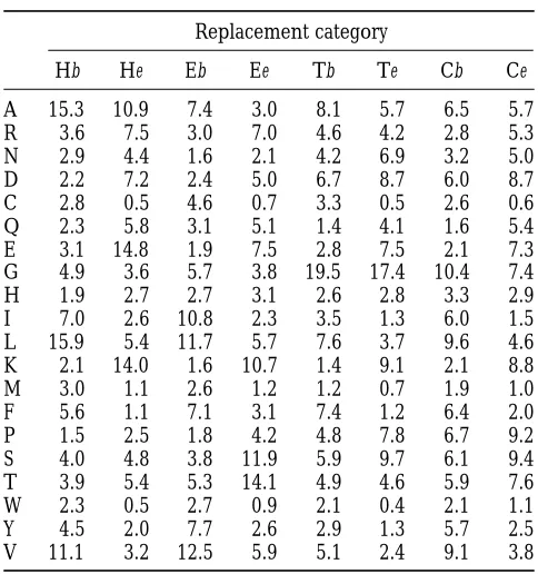
independent of the value of i. The conditional probabilities of transitions from Xyi to Wz1 are denoted aXy,Wz and were
A 15.3 10.9 7.4 3.0 8.1 5.7 6.5 5.7
estimated directly from the known structures in the BRKALN
R 3.6 7.5 3.0 7.0 4.6 4.2 2.8 5.3
database by their observed relative frequencies.
N 2.9 4.4 1.6 2.1 4.2 6.9 3.2 5.0
Given that the secondary structure of the next state is
identi-D 2.2 7.2 2.4 5.0 6.7 8.7 6.0 8.7
cal to that of the current state Xyi, we assume the accessibility
C 2.8 0.5 4.6 0.7 3.3 0.5 2.6 0.6
status of the next state is independent of i. The probability
Q 2.3 5.8 3.1 5.1 1.4 4.1 1.6 5.4
that the next site is buried, given that the current site is buried
E 3.1 14.8 1.9 7.5 2.8 7.5 2.1 7.3
and both sites have secondary structure X, is represented by
G 4.9 3.6 5.7 3.8 19.5 17.4 10.4 7.4
pX
b. The complementary probability qXb 5 12pXb is then the
H 1.9 2.7 2.7 3.1 2.6 2.8 3.3 2.9
probability that the next site is exposed, given that the current
site is buried and both sites have secondary structure X. Simi- I 7.0 2.6 10.8 2.3 3.5 1.3 6.0 1.5 larly, pX
e is the probability that the next site is exposed, given L 15.9 5.4 11.7 5.7 7.6 3.7 9.6 4.6
that the current site is exposed and both are secondary struc- K 2.1 14.0 1.6 10.7 1.4 9.1 2.1 8.8 ture X. We use qX
eto represent the complementary probability M 3.0 1.1 2.6 1.2 1.2 0.7 1.9 1.0
12pX
e. These probabilities are again estimated directly from F 5.6 1.1 7.1 3.1 7.4 1.2 6.4 2.0
the observed frequencies in the experimentally determined P 1.5 2.5 1.8 4.2 4.8 7.8 6.7 9.2
structures of the BRKALN database. S 4.0 4.8 3.8 11.9 5.9 9.7 6.1 9.4
Relative rates of amino acid replacement:One way to com- T 3.9 5.4 5.3 14.1 4.9 4.6 5.9 7.6 pare the eight estimated amino acid replacement processes W 2.3 0.5 2.7 0.9 2.1 0.4 2.1 1.1 is to determine the relative rate at which sites in the different
Y 4.5 2.0 7.7 2.6 2.9 1.3 5.7 2.5
replacement categories evolve. We normalize rates so that the
V 11.1 3.2 12.5 5.9 5.1 2.4 9.1 3.8
average site evolves at rate 1. First, note that the rate at which
amino acid i is replaced in category k isoj≠iakij, the sum of the Values listed are the parameterspkias described in the text,
replacement ratesak
ijover all amino acids that are not i. Second, given as percentages.
the overall replacement rate for category k isoipkioj≠iakij, which
accounts for amino acid frequencies by weighting the amino acid-specific rates by pk
i, the frequency of amino acid i in employed a nonparametric bootstrap resampling procedure
category k. Table 1 displays the estimated values of the pk
i. (EfronandTibshirani1993). One hundred resampled data
Finally, different replacement categories k have different sta- sets were constructed by sampling 207 randomly selected pro-tionary probabilities Ck, determined for our HMM by the tein families with replacement from the 207 families of the
equilibrium distribution of the matrixrij. Accounting for the BRKALN database. From each resampled data set, stationary
variation in stationary probabilities among replacement cate- probabilities of the eight replacement categories for our model gories, the relative rate of replacement for category k is were estimated. Likewise, replacement counts were generated from each resampled data set. Each resampled data set thereby Rk5 Rip
k iRj?iakij RlWlRipliRj?ialij
. (1)
TABLE 2 Relative replacement rates associated with a particular
second-ary structure averaged over accessibility classifications can also Relative rates of amino acid replacement be estimated. For example, the relative rate for helices is
Structure Buried Exposed Average
RH·5WHbRHb1WHeRHe
WHb1WHe Helix 0.7160.08 1.57 60.07 1.1160.06
0.7060.09 1.54 60.07 1.0960.07
5WHb(RipiHbRj?iaHbij )1WHe(RipHei Rj?iaHeij)
(WHb1WHe)RlWlRipl iRj?ialij
(2) Sheet 0.7260.05 1.20 60.18 0.8760.04
0.7160.06 1.18 60.17 0.8560.04 Similarly, relative rates for each accessibility classification aver- Turn 0.5660.05 1.30 60.09 1.0860.07 aged over secondary structures (e.g., R·b) can be estimated.
0.5560.05 1.28 60.08 1.0660.06 These estimates are shown in Table 2.
Coil 0.5160.03 1.23 60.06 0.9060.04 A concern is that one or a few proteins in the BRKALN
0.5060.03 1.35 60.12 0.9660.06 database could potentially have an especially large impact on
the relative rate estimates. The potential for a small number Average 0.6560.04 1.35 60.04 1 of protein families to have a great impact exists because the 0.6460.05 1.36 60.05 1 rate estimates are based upon amino acid replacement counts
from pairwise sequence comparisons. Protein families with many For each entry in the table, two pairs of rate estimates and sites or many sequences will tend to generate higher counts sample standard deviations are listed. The upper line of each that families consisting of a few short sequences. If these influ- entry refers to the case in which insertions relative to known ential protein families tend to evolve via comparatively atypical structures are ignored. The lower line refers to the case in evolutionary processes, the general applicability of our evo- which insertions relative to known structures are classified as
yielded estimates of relative rates of replacement for each To obtain the maximum likelihood estimate Tˆ , we use numeri-cal optimization algorithms (e.g., Swofford et al. 1996) to
category and the sample standard deviations of these estimates
were determined (see Table 2). determine the T that maximizes Pr(SuT). A slight improve-ment in model fit compared to our treatimprove-ment might be gener-A decision that we had to make when analyzing the pairwise
replacement count data was how to treat data from sites that ated via special consideration of secondary structure elements at the extreme carboxyl-terminus of proteins. For example, had unknown secondary structure or accessibility because they
were insertions relative to the experimentally determined column N of the alignment should not be the first position of an a-helix.
structure. One possibility was to ignore these data. Another
was to add these replacement count data to the exposed coil Prediction of protein secondary structure can subsequently be performed with a plug-in approach that fixes the tree at (Ce) replacement category because of the observed tendency
for insertion and deletion events to affect exposed coils. As Tˆ and uses appropriate methods to calculate the posterior distribution Pr(ciuS,Tˆ ). This has been described in more detail
the relative rate estimates in Table 2 exhibit, the treatments
yield similar outcomes. All other results presented here are for a simpler HMM of sequence evolution by Goldman et
al. (1996) and will be explored in the future for the HMM based on estimating rates by ignoring sites that are insertions
relative to known structures. introduced here.
Model comparisons:When a statistical comparison indicates Phylogenetic tree:Typically the form (topology and branch
lengths) of the phylogenetic tree relating a set of sequences that one evolutionary model is superior to a simpler model, this implies that features possessed by the complicated model is unknown but of interest. In this case, it may be treated as
a parameter of the problem and estimated using statistical and absent from the simple model may be evolutionarily im-portant. This approach has been taken in the past to compare methods. This is the approach that we adopt.
In protein structure prediction problems, it is now realized models of DNA sequence evolution (Goldman1993;Yanget
al. 1994, 1995), indicating the importance of factors such as that evolutionarily related amino acid sequences should not
be treated as though they are statistically independent of one base composition bias, transition/transversion rate ratio, and rate heterogeneity across DNA sites.
another (Benneret al. 1994;Goldmanet al. 1996). In fact,
common ancestry induces a correlation structure among se- In this study, we investigate models that range from the simplicity of sites evolving identically to the relative complexity quences that is specified by the phylogenetic tree relating
them. It has been shown that ideas developed in comparative of the full version of our new HMM in order to test the significance of the different components of the new model. We evolutionary biology (Felsenstein1985;HarveyandPagel
1991) for using phylogenetic trees to describe this correlation introduce the following notation to label the model variants. If structure can improve the results of secondary structure pre- the number of different secondary structure types recognized diction algorithms (Goldman et al. 1996). The model pre- is ss, the number of solvent accessibility classes distinguished
sented here provides a statistical basis for a protein secondary is acc, and the total number of states in the HMM is hmm, structure prediction technique that shares these benefits. then we can label models as ss/acc/hmm1(1indicating the Likelihood calculations:After estimating the relative rates use of the HMM to model dependencies between adjacent of replacementak
ij and the HMM transition probabilitiesrij sites) or ss/acc/hmm2(2indicating the disabling of the HMM;
from the BRKALN database, we can calculate the likelihood see below). Using this notation, our new HMM is denoted for a candidate phylogenetic tree T (representing both topol- 4/2/381. The following models were also considered: ogy and branch lengths). We do not re-estimate theak
ijorrij 1/1/12: This model represents the simplest case, in which
during the likelihood calculations but instead fix them at their no information on protein structure or nonindependence of estimated values. We denote the aligned data set by S, its sites is incorporated (hence, ss51 average secondary structure length (number of amino acids) by N, the first i columns of category, acc51 average accessibility state, and no meaningful the data set by Si, and the ith column itself by si. In the equa- HMM is possible). This corresponds to currently available
tions below, many of the probabilities are actually conditional methods implemented in software such as PAML (Yang1997)
uponak
ijandrijbut, for the sake of clarity, we omitakijandrij and MOLPHY (AdachiandHasegawa1995). We have
per-when this is feasible. The likelihood of the tree T is given by formed some analyses with each of three variants of this model: Pr(SuT), and this is calculated via the terms Pr(Si,ciuT) for each one derived from the work of Dayhoff et al. (1978) and
possible secondary structure category ci at site i using the denoted 1/1/1D2, one derived fromJoneset al. (1992) and
iteration: denoted 1/1/1J2, and the third derived from the BRKALN
database of this study and denoted simply 1/1/12. Pr(Si,ciuT )5
o
ci21
Pr(Si21,ci21uT)rci21ciPr(siuci,T ) (3) 4/2/81: This model adds to the 1/1/12model an HMM
recognizing four secondary structure elements, each with two for i.1. The terms Pr (siuci, T) are evaluated using the Markov accessibility categories. No special allowance is made for the
process replacement models appropriate for each secondary distributions of lengths of secondary structures (which there-structure ciand the pruning algorithm ofFelsenstein(1981). fore follow a purely geometric distribution under this model).
Because the site at the N terminus of a protein tends to be 4/1/191: This model adds to the 1/1/12model an HMM an exposed coil (Ce), we assume this is the case and start the recognizing four secondary structure elements and making iteration according to: allowance for the distributions of lengths of these structures
but does not recognize different solvent accessibilities. Pr(S1,c1uT )5Pr(s1uc1,T )Pr(c1uT)5Pr(s1uc1,T )dc1,Ce (4) For all the above models, the methods for estimating model
parameters varied slightly from those described above for the wheredc1,Ce51 if c15Ce, and 0 otherwise. This has proved 4/2/381 model because not all of the parameters of that slightly superior to using the stationary distribution (Ci) to model are meaningful for simpler versions. In all cases,
meth-describe the secondary structure probabilities at the first site
ods analogous to those described above for the 4/2/381model of sequences (results not shown), in which case Pr(S1, c1|T) were used to estimate appropriated parameters from the
is set equal to Pr(s1uc1,T )Cc1. When completed, the iteration BRKALN database (but see above regarding the 1/1/1/D2
gives the required Pr(SuT ) because and 1/1/1J2models); full details are available from the au-thors.
Pr(SuT)5
o
cN
Pr(SN,cNuT ). (5)
but sites are treated as independent of one another. This Alcohol dehydrogenase: Two data sets were formed from independence is achieved by replacing each row of the matrix the alignment available from the EBI ftp server, file (rij) with that matrix’s equilibrium distribution (Ci).
ds14642.dat (see alsoYokoyamaandHarry1993). The As with the 4/2/381 model (above), the 4/2/81 and
first (ADHAN) was formed from 16 mammalian, avian, 4/2/382models are implemented with the first site in a
pro-tein forced to be an exposed coil. For the 4/1/191model, and amphibian sequences, with the homologous se-accessibility status is not considered, and we simply treat the quence from the cod Gadus callarias added by the
au-first site as a coil. thors. The second (ADHPL) comprises 13 plant
se-quences.
Glutamate dehydrogenase (GDH): Eleven sequences, with
ANALYSIS OF EXAMPLE DATA SETS both eubacterial and eukaryotic representatives, were selected from the alignment file ds20281.dat (see also
Data sets: We analyzed 11 data sets that encompass
Telleret al. 1995). a broad range of genes, organisms, and evolutionary
G protein a subunit (GPA): Yokoyama andStarmer
divergence. When possible, we utilized previously
pub-(1992) aligned a large number of G proteinasubunit lished amino acid sequence alignments to reduce the
sequences (file ds15369.dat). We selected 18 Gia and chances that results could be biased by our own
align-Goa sequences from mammals, Drosophila melanogaster, ment procedures or prejudices. In addition, we selected
and Caenorhabditis elegans. sequences that were sufficiently similar to be likely to
Phosphoenolpyruvate carboxykinase (PEPCK): We have
share the same secondary structure.
used the alignment of 18 Lepidopteran sequences stud-Gapped positions in the alignments were treated as
ies and submitted (file ds24063.dat) byFriedlanderet missing information, as they are in the maximum
likeli-al. (1996).
hood programs of the PHYLIP package (Felsenstein
1995). In regions where the alignment was deemed rela- Model comparisons:Table 3 contains maximum log-tively unreliable, we treated the residues responsible for likelihoods obtained when analyzing each of the above the alignment difficulty as missing information. This 11 data sets with models ranging from the most simple was done to reduce the impact of alignment errors on (1/1/12, 1/1/1D2, 1/1/1J2) to the most complex the evaluation of our models. (4/2/381). To better understand which specific
fea-tures of our models are most responsible for improved
ADP-glucose pyrophosphorylase (abbreviated to ADPGP): Four
fits, we performed a series of parametric bootstrap analy-plant sequences were used, as analyzed by Goldman
ses on each data set. Each analysis was a comparison of andYang(1994) in a study of improved models of DNA
a relatively simple model (the null hypothesis H0) with nucleotide evolution.
a model that considers more aspects of protein structure
HIV-1 gp120 envelope glycoprotein (GP120): One
se-(the alternative hypothesis HA).
quence was selected from each of the eight major subtypes
We use a likelihood-ratio test with test statisticDl, the
(A–H) of HIV-1.
maximum log-likelihood for the alternative hypothesis
HIV-1 p17 matrix protein: Sequences were selected from
minus the maximum log-likelihood for the null hypoth-a number of strhypoth-ains of humhypoth-an immunodeficiency virus
esis. For the data sets analyzed here, this statistic can type 1 (HIV-1). Two data sets were studied, the first
be computed from the appropriate entries in Table 3. (P17ALL) comprising one sequence from each of the
To approximate the distribution of Dl under the null
seven subtypes (A–D, F–H) of HIV-1 for which
signifi-hypothesis, 100 simulated data sets are produced. The cantly different p17 sequences have been recognized
null model of sequence evolution is used, along with and the second (P17B) comprising eight sequences
the maximum likelihood topology and branch lengths from HIV-1 subtype B.
estimated under the null hypothesis for the original
Sucrose synthase (SUSY): Four dicotyledonous plant
se-data set, to generate each simulated se-data set. The simu-quences were used, as analyzed in a preliminary study
lated data sets have the same number of taxa and are of the effects on protein structure on sequence
evolu-the same length as evolu-the original data set. If a residue at tion byThorneet al. (1996).
a particular site in the data set has unknown type in the
Xylanase (XYLA): Seven prokaryotic sequences were
original data set because of alignment uncertainty or used, as analyzed in a preliminary study of
phylogeny-gaps, the residue at this position is also considered un-and likelihood-based methods of protein secondary
known in the simulated data set. For each simulated structure prediction byGoldmanet al. (1996).
data set,Dl can be calculated via likelihood
maximiza-tion under the null and alternative hypotheses. If the The following five data sets were derived from
multi-ple sequence alignments deposited at the EMBL-Euro- observed value of Dl for the original data set is
suffi-ciently extreme relative to the distribution of simulated pean Bioinformatics Institute (EBI) and available
elec-tronically from ftp://ftp.ebi.ac.uk/pub/databases/embl/ values, then the null hypothesis can be rejected. One measure of extremity is given by the proportion of simu-align. In each case, minor alterations were made by
TABLE 3
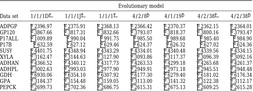
Maximum log-likelihoods for the analysis of 11 data sets under seven model variants
Evolutionary model
Data set 1/1/1D2 1/1/1J2 1/1/12 4/2/81 4/1/191 4/2/382 4/2/381
ADPGP 22396.97 22375.91 22368.13 22366.42 22370.37 22362.15 22364.01 GP120 23867.66 23817.31 23832.66 23793.07 23818.37 23800.16 23793.47 P17ALL 21009.89 2990.04 2991.75 2985.50 2989.68 2985.40 2984.90 P17B 2632.59 2627.12 2629.46 2624.37 2626.32 2627.02 2624.36 SUSY 24401.75 24348.94 24343.29 24334.01 24340.48 24339.56 24334.15 XYLA 23162.47 23144.63 23127.90 23093.86 23117.37 23096.39 23092.16 ADHAN 24366.52 24340.12 24317.73 24263.53 24299.18 24265.68 24261.37 ADHPL 23002.63 22993.03 22977.90 22949.91 22971.18 22945.51 22948.48 GDH 26930.06 26354.10 26307.92 26177.30 26279.40 26181.02 26176.34 GPA 23184.37 23154.48 23159.05 23113.00 23141.32 23122.38 23112.17 PEPCK 22699.73 22702.36 22686.75 22615.31 22675.13 22609.25 22615.28
value. This proportion is an estimate of the probability son between a null hypothesis of the 4/2/81 model and the 4/2/381model focuses on modelling realistic under H0of realizing a value ofDl at least as extreme as
that observed for the original data. Sufficiently low values length distributions for secondary structure. We found it also of interest to use the 4/1/191, 4/2/382, imply rejection of H0. Another measure of extremity is a
z-score, calculated by subtracting the mean simulated test 4/2/81, and 4/2/381models as alternative hypotheses
when the 1/1/12model was the null hypothesis. These statistic value from the actual value and then dividing by
the sample standard deviation of the simulated values. comparisons explore how much various combinations of the aforementioned four features improve upon a In our parametric bootstrap comparisons, we do not
account for uncertainty in parameters governing the model that neglects structure. The results of these para-metric bootstrap comparisons are shown in Table 4. relative rates of amino acid replacement or organization
of secondary structure and solvent accessibility. Esti- Computation times: Because of the 38 HMM states and the eight replacement categories, our 4/2/381 mates for these parameters are fixed at the values
ob-tained from the BRKALN database. Only the topology model is more computationally demanding than the 1/1/12model. Our experience is that the computation and branch lengths are estimated from the simulated
data sets. Ideally, the parametric bootstrap procedure time required for analyzing data sets is more sensitive to the number of replacement categories than to the would account for the uncertainty in all parameters
when comparing models, but this would be computation- number of HMM states. For this reason, one might expect the 4/2/381 model to require approximately ally expensive.
Parametric bootstrap comparisons between some eight times more computation than the 1/1/12model. In our experience, the actual ratio of CPU times re-models are more informative than those between
oth-ers. By combining evolution with protein structure, four quired by these two models varies somewhat between analyses. As an example, in a case where topology was potentially important features that we have incorporated
in the 4/2/381model are (1) association of secondary fixed and branch lengths were estimated, analysis of the GPA data set on a Digital Alphastation 500/400 required structure and amino acid replacement dynamics, (2)
association of solvent accessibility and replacement dy- 199 seconds of CPU time with the 1/1/12 model and 943 seconds with the 4/2/381model.
namics, (3) regional organization of secondary structure and solvent accessibility along a sequence, and (4) a relatively realistic length distribution of secondary
struc-DISCUSSION ture elements. Earlier work (Thorneet al. 1996)
indi-cated that the effect of secondary structure on amino An earlier study (Thorneet al. 1996) that considered just three structure categories (a-helix, b-sheet, and acid replacement is important. Therefore, we have
con-centrated on parametric bootstrap analyses that assess the loop) demonstrated that consideration of secondary structure can significantly improve the fit of models to remaining three features. The comparison between a null
hypothesis of the 4/1/191model and the 4/2/381model data. The belief that secondary structure is important is reinforced by the results shown in Table 4. All but investigates the effect of solvent accessibility on amino
acid replacement. The comparison between a null hy- one of the comparisons in which the null hypothesis makes no distinction between secondary structures and pothesis of the 4/2/382model and the 4/2/381model
compari-TABLE 4
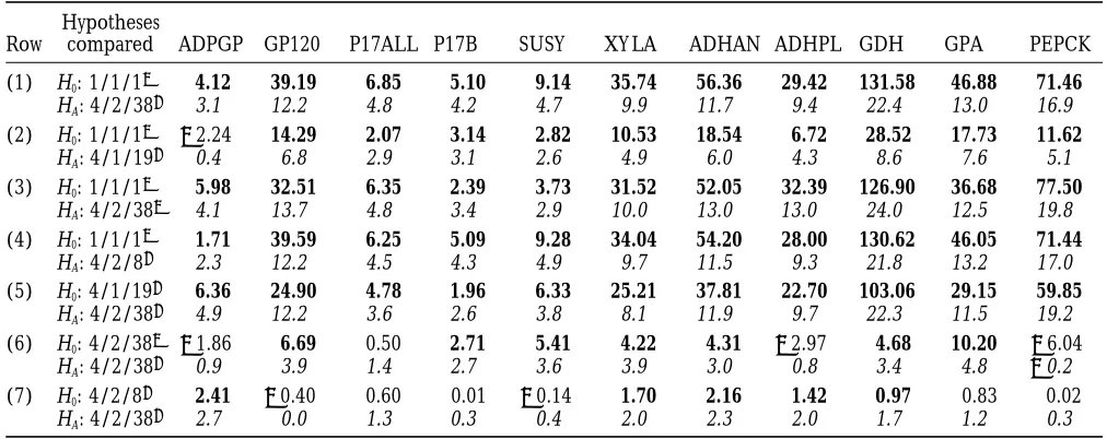
Results of parametric bootstrap analyses
Hypotheses
Row compared ADPGP GP120 P17ALL P17B SUSY XY LA ADHAN ADHPL GDH GPA PEPCK
(1) H0: 1/1/12 4.12 39.19 6.85 5.10 9.14 35.74 56.36 29.42 131.58 46.88 71.46
HA: 4/2/381 3.1 12.2 4.8 4.2 4.7 9.9 11.7 9.4 22.4 13.0 16.9
(2) H0: 1/1/12 22.24 14.29 2.07 3.14 2.82 10.53 18.54 6.72 28.52 17.73 11.62
HA: 4/1/191 0.4 6.8 2.9 3.1 2.6 4.9 6.0 4.3 8.6 7.6 5.1
(3) H0: 1/1/12 5.98 32.51 6.35 2.39 3.73 31.52 52.05 32.39 126.90 36.68 77.50
HA: 4/2/382 4.1 13.7 4.8 3.4 2.9 10.0 13.0 13.0 24.0 12.5 19.8
(4) H0: 1/1/12 1.71 39.59 6.25 5.09 9.28 34.04 54.20 28.00 130.62 46.05 71.44
HA: 4/2/81 2.3 12.2 4.5 4.3 4.9 9.7 11.5 9.3 21.8 13.2 17.0
(5) H0: 4/1/191 6.36 24.90 4.78 1.96 6.33 25.21 37.81 22.70 103.06 29.15 59.85
HA: 4/2/381 4.9 12.2 3.6 2.6 3.8 8.1 11.9 9.7 22.3 11.5 19.2
(6) H0: 4/2/382 21.86 6.69 0.50 2.71 5.41 4.22 4.31 22.97 4.68 10.20 26.04
HA: 4/2/381 0.9 3.9 1.4 2.7 3.6 3.9 3.0 0.8 3.4 4.8 20.2
(7) H0: 4/2/81 2.41 20.40 0.60 0.01 20.14 1.70 2.16 1.42 0.97 0.83 0.02
HA: 4/2/381 2.7 0.0 1.3 0.3 0.4 2.0 2.3 2.0 1.7 1.2 0.3
As described in the text, seven different hypothesis tests (rows 1–7) were performed for each of 11 data sets. Two entries are listed for each combination of hypothesis test and data set. These entries are the following: (upper) the observed value ofDl, the log-likelihood for HAminus the log-likelihood for H0, and (lower) a z-score (italic type) that measures the estimated number
of standard deviations by which the observed value ofDl exceeds the mean of the simulated values. When fewer than 5 of 100 simulatedDl values equal or exceed the observed value, the observedDl value is shown in bold type.
tures strongly reject the null hypothesis (Table 4, rows structure categories along sequences. For some data sets, the null hypothesis of no correlation could not be 1–4). Further evidence for an association between
sec-ondary structure and amino acid replacement is summa- rejected. This could reflect failure of the 4/2/381 model to incorporate information from residues that rized in Table 2. We note the surprising results that the
estimated rates for buried helix and sheet residues are are not close in the linear sequence. Methods for de-tecting long-range interactions in an evolutionary con-greater than those for buried turns and coils and that
the estimated rate for exposed helix residues is greater text are currently being developed (D. D. Pollock, unpublished results), and we hope that the information than those for other exposed residues. Because the
probability a site has a particular accessibility status is they yield can be incorporated into models used for phylogenetic inference. An alternative explanation for not independent of its secondary structure, these
pat-terns are less clear for the weighted average over buried failing to reject the null hypothesis of no correlation is that some data sets may have too few sequences or too and exposed sites. Nevertheless, it is still contrary to
intuition thata-helix andb-sheet positions experience little evolutionary divergence to provide relative cer-tainty about underlying structural environments. It is more amino acid replacements on average than coil
positions. difficult to detect regional organization of structure along a sequence if there is a high degree of uncertainty Differences in amino acid replacement dynamics
asso-ciated with solvent accessibility status have been ex- regarding the underlying structural environment at each site.
plored by KoshiandGoldstein(1995), but their
sig-nificance to protein evolution has not been statistically We have preliminary indications that secondary struc-ture predictions generated from our 4/2/381 model tested. In our study, the tests represented in Table 4,
rows 1, 3, 4, and 5, have a bearing on this question. are superior to those from the 4/2/382 model. For example, predictions of the 4/2/382model exhibit an Rows 1, 3, and 4 represent tests in which the effect of
accessibility is studied in combination with other com- abundance of unrealistically shorta-helices andb-sheets (results not shown). It may be the case that incorporat-ponents of the models. The comparison between the
4/1/191and 4/2/381models (Table 4, row 5) directly ing correlation of structure categories will be important for accurate secondary structure prediction, even for investigates the effect of incorporating accessibility into
our evolutionary model. For every data set and for all of data sets where it has little impact on the goodness of fit of models. This possibility will be a focus of future these tests, the model incorporating solvent accessibility
information is strongly preferred. research.
For six of the 11 data sets, we find that the comparison The comparison of the 4/2/382and 4/2/381models
re-ject the former. For these data sets, there is no signifi- evolutionary processes of globular and membrane pro-teins are apt to differ, and Jones et al. (1994) have cant evidence in favor of the more complex HMM that
attempts to use information regarding the distribution demonstrated that patterns of amino acid replacement in integral membrane proteins bear little resemblance of lengths of secondary structure elements. Mixed
re-sults across different data sets (Table 4, row 7) again to those in globular proteins.
In this article we have described the analysis of amino make it unclear whether this is a failing of our model
or is due to insufficient data. Detection of both struc- acid sequences under the assumption that the protein’s true structure is unknown. In the case that the tertiary tural correlation along sequences and information
per-taining to the length distributions of secondary struc- structure has been determined for a protein, the phylo-genetic estimation method can be modified to allow the ture elements might be assisted by adding more
sequences to a data set. This should in effect increase known secondary structure and accessibility informa-tion to be used. This would remove some of the sources the information pertaining to each alignment position
and make the HMM states “less hidden.” of uncertainty and should improve the estimation of phylogenies. In this way, experimentally determined Improved models of sequence evolution can lead to
improved estimates of both evolutionary relationships structures could directly assist phylogenetics instead of being ingored, or being used indirectly through their (topology) and distances (branch lengths) in
phyloge-nies (e.g.,Yanget al. 1994).NaylorandBrown(1997) influence on average properties of databases of known structures as in this article.
have recently illustrated adverse effects on phylogenetic
tree estimation from mammalian mitochondrial protein Our amino acid replacement models for the eight structural environment categories are based only on sequences when physicochemical properties of amino
acids are ignored. We hope that our new (4/2/381) analysis of database sequences. They are not varied to suit specific proteins. A promising approach for tai-model may give more reliable phylogenetic estimates
than simpler models. It directly incorporates four com- loring amino acid replacement processes to specific pro-teins has been developed by Caoet al. (1994) for an ponents representing structural features that have not
generally been considered in models of sequence evolu- evolutionary model that ignores protein structure. This technique combines parameters estimated from data-tion, instead of using physicochemical properties of
amino acids as surrogates. Two of these components, base sequences with amino acid frequencies calculated from the specific sequences being analyzed and poten-encompassing effects of secondary structure and
accessi-bility, give particularly large improvements in the fit of tially could be extended to models that consider protein structure.
models across the broad range of data sets that were
studied. All models are potentially misled by violations of their assumptions. Our model assumes that all residues of One result ofNaylorand Brown(1997) seems to
contradict our finding that buried sites evolve more an alignment are related via the same phylogeny, for example, that recombination is absent, but the HIV-1 slowly than exposed sites.NaylorandBrownclassified
sites as hydrophilic or hydrophobic on the basis of the data sets we have analyzed have potentially been subject to intra- and interspecific recombination (Robertson amino acids found in the alignment column at that site.
In the data sets we analyzed, hydrophilic sites tend to et al. 1995). Additionally, although structure is more
conserved than sequence (e.g.,ChothiaandLesk1986; be exposed to solvent and hydrophobic sites tend to be
buried. With a parsimony analysis,NaylorandBrown Russellet al. 1997), it clearly does evolve. For example, there is some evidence that the secondary structure of (1997) concluded that hydrophilic sites fit an accepted
tree topology better than hydrophobic sites. We attri- one of the proteins we have examined (GP120) can vary in different strains of HIV-1 (Hansenet al. 1996). Our bute this difference in fit (as measured by parsimony
techniques) to heterogeneity of rates among sites: slowly model currently assumes that there has been no change in protein secondary structure or accessibility since se-evolving sites generate less homoplasy than quickly
evolving sites. Therefore, their results could be ex- quence divergence. Advanced models that explicitly ad-dress the evolution of structure would be of great inter-plained if, in contrast to our results, hydrophobic
(bur-ied) sites were evolving more quickly on average than est for phylogenetic estimation, structure prediction, and the study of evolutionary processes. Although this hydrophilic (exposed) sites.
Fortunately, the two studies can be reconciled by real- would add complexity to our model, modern computa-tional statistical methods may make such developments izing that our work is based on experimentally
deter-mined structures that are exclusively globular proteins practical.
One of the most important advances in the recon-whereasNaylorandBrown(1997) studied only
inte-gral membrane proteins. Relatively unconstrained sites struction of evolutionary trees has been the consid-eration of heterogeneity of evolutionary rates among on the surface of a globular protein are apt to be
ex-posed to solvent and hydrophilic, but the relatively un- sequence sites (e.g., Yang 1994, 1996). Although this variability has been statistically modelled, typically with a constrained sites on the surface of a membrane protein
and Structure, edited byM. O. Dayhoff. National Biomedical
well characterized. Our estimates (Table 2) indicate that
Research Foundation, Washington, DC.
rate heterogeneity is strongly associated with structural Dayhoff, M. O., R. M. SchwartzandB. C. Orcutt,1978 A model
environment. Exposed sites tend to experience z23 of evolutionary change in proteins, pp. 345–352 in Atlas of Protein
Sequence and Structure, edited byM. O. Dayhoff.National
Biomed-the rate of amino acid replacements experienced by
ical Research Foundation, Washington, DC.
buried sites. A higher rate of replacement for exposed Efron, B.,andR. J. Tibshirani,1993 An Introduction to the Bootstrap.
sites is seen for each secondary structure type. The asso- Chapman and Hall, New York.
Felsenstein, J.,1981 Evolutionary trees from DNA sequences: a
ciation between accessibility status and replacement
maximum likelihood approach. J. Mol. Evol. 17: 368–376.
rates is a noteworthy feature of protein evolution but Felsenstein, J., 1985 Phylogenies and the comparative method.
has received scant attention in the field of molecular Am. Nat. 125: 1–15.
Felsenstein, J., 1995 PHYLIP (Phylogenetic Inference Package), Ver.
evolution and has not been previously exploited in
phy-3.57. Department of Genetics, University of Washington, Seattle.
logenetic studies. Felsenstein, J.,andG. A. Churchill,1996 A hidden Markov model We believe that characterizing general associations of approach to variation among sites in rate of evolution. Mol. Biol.
Evol. 13: 93–104.
patterns and rates of sequence evolution with
pheno-Friedlander, T. P., J. C. Regier, C. MitterandD. L. Wagner,1996
typic features such as protein structure is essential to A nuclear gene for higher-level phylogenetics—phosphoenolpy-understanding the process of sequence evolution both ruvate carboxykinase tracks Mesozoic-age divergences within
Lepid-optera (Insecta). Mol. Biol. Evol. 13: 594–604.
within and between populations. It is the relationship
Goldman, N.,1993 Statistical tests of models of DNA substitution.
between genotype and phenotype that drives much of J. Mol. Evol. 36: 182–198.
evolution. Protein structure is fundamental to pheno- Goldman, N.,andZ. Yang,1994 A codon-based model of nucleotide
substitution for protein-coding DNA sequences. Mol. Biol. Evol.
type and yet little previous effort has been devoted to
11:725–736.
characterizing its impact on evolution.
Goldman, N., J. L. ThorneandD. T. Jones,1996 Using evolutionary
trees in protein secondary structure prediction and other
compar-Edward Holmeskindly assisted with the HIV-1 data sets. We also
ative sequence analyses. J. Mol. Biol. 263: 196–208. thankDavid Pollock, Pietro Lio` ,and two anonymous referees for
Gotoh, O.,1982 An improved algorithm for matching biological
their helpful suggestions. N.G. is supported by a Wellcome Trust
sequences. J. Mol. Biol. 162: 705–708. Fellowship in Biodiversity Research. J.L.T. was supported by
Na-Hansen, J. E., O. Lund, J. O. Nielsen, S. BrunakandJ.-E. S.
Han-tional Institutes of Health grant P01-GM45344 and the Alfred P. Sloan
sen,1996 Prediction of the secondary structure of HIV-1 gp120.
Foundation. D.T.J. is supported by a Royal Society University Re- Proteins 25: 1–11.
search Fellowship. Software, parameter estimates, and data sets used Harvey, P. H.,andM. D. Pagel,1991 The Comparative Method in
for the analysis described above are available from the authors via Evolutionary Biology. Oxford University Press, Oxford, UK. http://ng-dec1.gen.cam.ac.uk/hmm/contents.html. Hasegawa, M., H. Kishinoand T. A. Yano,1985 Dating of the
human-ape splitting by a molecular clock of mitochondrial DNA. J. Mol. Evol. 22: 160–174.
Jones, D. T., W. R. TaylorandJ. M. Thornton,1992 The rapid
LITERATURE CITED generation of mutation data matrices from protein sequences.
CABIOS 8: 275–282.
Adachi, J.,andM. Hasegawa,1995 MOLPHY: Programs for Molecular
Jones, D. T., W. R. TaylorandJ. M. Thornton,1994 A mutation
Phylogenetics, Ver. 2.3. Institute of Statistical Mathematics, Tokyo. data matrix for transmembrane proteins. FEBS Letts. 339: 269–
Asai, K., S. HayamizuandK. Handa,1993 Prediction of protein
275. secondary structure by the hidden Markov model. CABIOS 9:
Jukes, T. H.,andC. R. Cantor,1969 Evolution of protein
mole-141–146.
cules, pp. 21–132 in Mammalian Protein Metabolism, edited by
Benner, S. A., I. Badcoe, M. A. Cohenand D. L. Gerloff,1994
H. N. Munro.Academic Press, New York.
Bona fide prediction of aspects of protein conformation: assigning
Kabsch, W.,andC. Sander,1983 Dictionary of protein secondary
interior and surface residues from patterns of variation and
con-structure: pattern recognition of hydrogen bonded and geometri-servation in homologous sequences. J. Mol. Biol. 235: 926–958.
cal features. Biopolymers 22: 2577–2637.
Bernstein, F. C., T. F. Koetzle, G. J. B. Williams, E. F. Meyer,
Kimura, M., 1983 The Neutral Theory of Molecular Evolution. Cam-M. D. Brice et al., 1977 The protein data bank: a
computer-bridge University Press, Camcomputer-bridge, UK. based archival file for macromolecular structures. Eur. J.
Bio-Koshi, J. M.,andR. A. Goldstein,1995 Context-dependent optimal
chem. 80: 319–324.
substitution matrices. Prot. Eng. 8: 641–645.
Bleasby, A. J.,andJ. C. Wootton,1990 Construction of validated,
Lu¨ thy, R., A. D. McLachlanandD. Eisenberg,1991 Secondary
non-redundant composite protein sequence databases. Prot. Eng.
structure-based profiles: use of structure-conserving scoring
ta-3:153–159.
bles in searching protein sequence databases for structural
simi-Brown, M., R. Hughey, A. Krogh, I. S. Mian. K. Sjolanderet al.,
larities. Proteins 10: 229–239. 1993 Using Dirichlet mixture priors to derive hidden Markov
Naylor, G. J. P.,andW. M. Brown,1997 Structural biology and
models for protein families, pp. 47–55 in Proceedings of the First
phylogeny estimation. Nature 388: 527–528.
International Conference on Intelligent Systems for Molecular Biology,
Overington, J., M. S. Johnson, A. S˘aliandT. L. Blundell,1990
edited byL. Hunter, D. SearlsandJ. Shavlik.AIII Press, Menlo
Tertiary structural constraints on protein evolutionary diversity: Park, CA.
templates, key residues and structure prediction. Proc. R. Soc.
Bruno, W. J.,1996 Modelling residue usage in aligned protein
se-Lond. Ser B 241: 132–145. quences via maximum likelihood. Mol. Biol. Evol. 13: 1368–1374.
Robertson, D. L., B. H. HahnandP. M. Sharp,1995 Recombina-Cao, Y., J. Adachi, A. Janke, S. Pa¨ a¨ boandM. Hasegawa,1994
Phy-tion in AIDS viruses. J. Mol. Evol. 40: 249–259. logenetic relationships among eutherian orders estimated from
Russell, R. B., M. A. S. Saqi, R. A. Sayle, P. A. BatesandM. J. E.
inferred sequences of mitochondrial proteins: instability of a tree
Sternberg,1997 Recognition of analogous and homologous
based on a single gene. J. Mol. Evol. 39: 519–527.
protein folds: analysis of sequence and structure conservation. J.
Chothia, C.,andA. M. Lesk,1986 The relation between the
diver-Mol. Biol. 269: 423–439. gence of sequence and structure in proteins. EMBO J. 5: 823–826.
Swofford, D. L., G. J. Olsen, P. J. WaddellandD. M. Hillis,1996 Churchill, G. A.,1989 Stochastic models for heterogeneous DNA
Phylogenetic inference, pp. 407–514 in Molecular Systematics, Ed. sequences. Bull. Math. Biol. 51: 79–94.
2, edited byD. M. Hillis, C. MoritzandB. K. Mable.Sinauer Dayhoff, M. O., R. V. EckandC. M. Park,1972 A model of
Taylor, W. R.,1988 A flexible method to align large numbers of Yang, Z.,1994 Maximum likelihood phylogenetic estimation from
DNA sequences with variable rates over sites: approximate meth-biological sequences. J. Mol. Evol. 28: 161–169.
Teller, J. K., P. J. Baker, K. L. Britton, P. C. Engel, D. W. Riceet ods. J. Mol. Evol. 39: 306–314.
Yang, Z.,1995 A space-time process model for the evolution of DNA
al., 1995 Correlation of intron-exon organisation with the
three-dimensional structure in glutamate dehydrogenase. Biochim. Bio- sequences. Genetics 139: 993–1005.
Yang, Z.,1996 Among-site rate variation and its impact on
phyloge-phys. Acta 1247: 231–238.
Thorne, J. L., N. GoldmanandD. T. Jones,1996 Combining pro- netic analysis. TREE 11: 367–372.
Yang, Z.,1997 PAML: a program package for phylogenetic analysis
tein evolution and secondary structure. Mol. Biol. Evol. 13: 666–
673. by maximum likelihood. CABIOS 13: 555–556.
Yang, Z., N. GoldmanandA. Friday,1994 Comparison of models Topham, C. M., A. McLeod, F. Eisenmenger, J. P. Overington, M. S.
Johnsonet al., 1993 Fragment ranking in modelling of protein for nucleotide substitution used in maximum-likelihood
phyloge-structure: conformationally constrained substitution tables. J. netic estimation. Mol. Biol. Evol. 11: 316–324.
Mol. Biol. 229: 194–220. Yang, Z., I. J. LauderandH. J. Lin,1995 Molecular evolution of Wako, H.,andT. L. Blundell,1994 Use of amino acid environ- the hepatitis B virus genome. J. Mol. Evol. 41: 587–596.
ment-dependent substitution tables and conformational propen- Yokoyama, S.,andW. T. Starmer,1992 Phylogeny and evolutionary
sities in structure prediction from aligned sequences of homolo- rates of G proteinasubunit genes. J. Mol. Evol. 35: 230–238. gous proteins. I. Solvent accessibility classes. J. Mol. Biol. 238: Yokoyama, S., and D. E. Harry,1993 Molecular phylogeny and
682–692. evolutionary rates of alcohol dehydrogenases in vertebrates and
White, J. V., C. M. StultzandT. F. Smith,1994 Protein classifica- plants. Mol. Biol. Evol. 10: 1215–1226.
tion by stochastic modeling and optimal filtering of amino-acid