Precision mapping of quantitative trait loci.

(1)

Copyright 0 1994 by the Genetics Society of America

Precision Mapping of Quantitative Trait Loci

Zhao-Bang Zeng

Program in Statistical Genetics, Department of Statistics, North Carolina State University, Raleigh, North Carolina 27695-8203

Manuscript received June 30, 1993 Accepted for publication December 15, 1993

ABSTRACT

Adequate separation of effects of possible multiple linked quantitative trait loci (QTLs) on mapping QTLs is the key to increasing the precision of QTL mapping. A new method of QTL mapping is proposed and analyzed in this paper by combining interval mapping with multiple regression. The basis of the proposed method is an interval test in which the test statistic on a marker interval is made to be unaffected by QTLs located outside a defined interval. This is achieved by fitting other genetic markers in the statistical model as a control when performing interval mapping. Compared with the current QTL mapping method ( i . e . , the interval mapping method which uses a pair or two pairs of markers for mapping QTLs), this method has several advantages. (1) By confining the test to one region at a time, it reduces a multiple dimensional search problem (for multiple QTLs) to a one dimensional search problem. (2) By conditioning linked markers in the test, the sensitivity of the test statistic to the position of individual QTLs is increased, and the precision of QTL mapping can be improved. (3) By se- lectively and simultaneously using other markers in the analysis, the efficiency of QTL mapping can be also improved. The behavior of the test statistic under the null hypothesis and appropriate critical value of the test statistic for an overall test in a genome are discussed and analyzed. A simulation study of QTL mapping is also presented which illustrates the utility, properties, advantages and disadvantages of the method.

M

ANYtraits in plants and animals are quantitative in nature, influenced by many genes. It has been, for a long time, an important aim in genetics and breeding to identify those genes contributing significantly to the variation of traits within and between populations or species. With rapid advancement of molecular technol- ogy, it is now possible to use molecular marker information to map major quantitative trait loci (QTLs) on chromosomes ( e . g . , PATERSON et al. 1988,1991; HILBERT et al. 1991; JACOB et al. 1991; STUBER et al. 1992).

There have been several statistical methods developed to analyze mapping data to search systematically for major QTLs in experimental organisms ( e . g . , SOLLER et ul.

1976; WELLER 1986; LANDER and BOTSTEIN 1989), among which the interval mapping of LANDER and

BOTSTEIN

(1989) has now become the current standard method

used by many geneticists for mapping QTLs. Compared with the traditional method (SOLLER et al. 1976), the interval mapping method has a number of advantages. But it still has several problems, particularly in distinguishing multiple linked QTL effects. When there are two or more QTLs located on a chromosome, the m a p ping of QTLs can be seriously biased, and QTLs can be mapped to wrong positions (KNOTI. and HALEY 1992; MARTINEZ and CURNOW 1992).

To increase the reliability and accuracy of QTL m a p ping, the effects of possible multiple linked QTLs on a chromosome should be adequately separated in testing and estimation. In this paper, a mapping procedure is

Genetics 136: 1457-1468 (April, 1994)

elaborated with the aim to improve both the precision and efficiency of mapping multiple QTLs, using multiple markers. The basis of the method is an interval test in which the test statistic is constructed to be unaffected by QTLs located outside a defined interval. This is achieved by using the properties of multiple regression analysis (ZENG 1993). Although multiple regression analysis has been used for mapping QTLs ( COWEN 1989; STAM 1991), the theoretical properties of multiple regression analysis in relation to QTL mapping were analyzed in detail only recently by ZENG (1993) and also independently by RODOLPHE and LEFORT (1993). More- over, ZENG (1993) proposed to utilize these properties to construct a composite interval mapping method to improve the precision and efficiency of mapping QTLs. Recently, JANSEN (1993) also proposed a procedure to combine interval mapping with multiple regression for mapping QTLs. There are some similarities and also differences between the method analyzed in ZENG (1993) and here and that proposed byJANSEN (1993). These are discussed at the end of this report.

(2)

1458 Z.3. Zeng

BACKGROUND AND PROBLEMS

Data type: Data for mapping QTLs consist of marker

information (marker types for a number of polymorphic markers) and quantitative trait values for a number of individuals. Marker types for each marker can be re- corded in digital form, such as 1 and 0 for distinguishing the two marker types (homozygote and heterozygote) for a backcross population from two inbred lines, and 2, 1 and 0 for distinguishing the three marker types (homozygote, heterozygote and another homozygote) for an F2 population from two inbred lines. Based on seg- regation analysis, these markers can usually be ordered in linkage groups or are located linearly on chromosomes.

Traditional method-simple linear regression: The sim- plest method of associating markers with quantitative trait variation is to test for trait value differences between different marker groups of individuals for a particular marker ( e . g . , SOLLER et al. 1976). For example, if we let

PM,/Ml

and

pM,/M,

be the observed trait means of the groups of individuals with marker genotypes M , / M , and M , / M 2 for a particular marker in a backcross population, we can test for significance between means

pM1/*,,

and

PM,/,,,,,

using the usual t test. The hypotheses under the test can be

Ho: P M , / M , = P M , / ~ I ~ and HI: P M , / M , f PM,/M,.

Statistically, this is equivalent to the simple regression analysis with a model

y I = b o + bxI+ ej j = 1 , 2 ,

. . . ,

n (1)

where y, is the trait value of the jth individual in a population, 6, is the mean (a parameter) in the model, xj is a dummy variable for the jth individual, taking a value of 1 for marker type M , / M , and 0 for marker type M,/

M2, b =

pMl/M,

- P,,,,~~ is the simple regression coef-

ficient, and ej is a random residual variable for the jth individual. A test can be performed in this model on the regression coefficient.

To understand the relevance of this test to QTL mapping, we need to know what exactly is tested in genetic terms. Suppose that there are m QTLs contributing to the genetic variation in a backcross population from two inbred lines. Genetically the expected difference between

l-%”

,MI and P M , ,My is

m

& ( P M , / M , - P M l / M 2 ) =

C.

(1 - 2ri)at (2)

1= 1

ignoring epistasis, where E denotes expectation, ai is the effect of the ith QTL expressed as a difference between the recurrent parent homozygote and the heterozygote, and r, is the recombination frequency between the ith QTL and the marker. This means that essentially we are testing a composite parameter that

constitutes gene effects and recombination frequen- cies for (potentially) a number of genes. Of course, many QTLs may not be linked to the marker and thus have 0.5 recombination frequency. The above hypotheses are then equivalent to

H,: all r, = 0.5 and HI: at least one ri < 0.5,

because ai’s are assumed to be non-zero (i. e . , by ex- periment we know that there are some genes which are segregating in the population). If

PMl/,+fl

and are found to be significantly different, it is indicated that the marker is linked to one or possibly more QTLs.

Although simple, this analysis captures the basic ideas of QTL mapping. Clearly there are many problems with this simple approach (LANDER and BOTSTEIN 1989), such as: (i) the method cannot tell whether the markers are associated with one or more QTLs, (ii) the method does not estimate the likely positions of the QTLs, (iii) the effects of QTLs are likely to be underestimated because they are confounded with the recombination frequen- cies and (iv) because of the confounding effects, the method is not very powerful and many individuals are required for the test.

LANDER and BOTSTEIN’S interval mapping: If there is only one QTL on a chromosome, LANDER and BOTSTEIN

(1989) proposed the use of a pair of markers to disen- tangle r and a from the test statistic. Specifically, for a backcross design they proposed the following linear model to test for a QTL located on an interval of markers

i and i

+

1

y, = bo

+

b*xT

+

eI j = 1, 2 , .

. .

, n (3)

where b* is the effect of the putative QTL expressed as a difference in effects between the homozygote and heterozygote, xTis an indicator variable, taking a value 1 or 0 with probability depending on the genotypes of markers i and i

+

1 and the position being tested for the putative QTL (Table 1). Statistically this is a mixture model (TITTERINGTON et al. 1985; MCLACHLAN and BAS-

FORD 1988). By using the property and procedures of

mixture model analysis, Lander and Botstein built up a likelihood ratio test based on the hypotheses

H,: 6* = 0 and H,: 6” f 0

(3)

Mapping Quantitative Trait Loci 1459

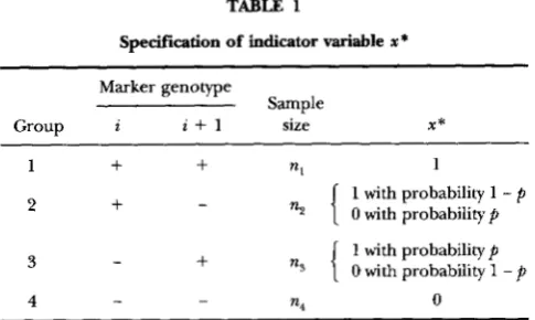
TABLE 1

Specification of indicator variable x *

Marker genotype

Sample

Group i i + l size X *

1

+

nl 1

2

+

-

n2

{

ns

1

1 with probability 1 - p

0 with probability p

1 with probability p

0 with probability 1 -

p

3

4

-

+

- -

n4 0

+

denotes homozygote of the marker genotype and - denotes heterozygote. In analysis,

p

can be treated either as a parameter or as a constant with p = r , q / r z ( t + l ) , where r,, is the recombination frequency between marker i and the position q being tested for a putative QTL and ri(z+,) is the recombination frequency between markers

i and i

+

1. Double recombination within the marker interval is

ignored.

BOTSTEIN 1989). By the property of the maximum likelihood analysis, the estimates of locations and effects of QTLs are asymptotically unbiased if the assumption that there is at most one QTL on a chromosome is true. They also suggested methods to increase the power of QTL mapping, notably the selective genotyping of the extreme progeny.

Compared with the traditional method, the interval mapping method has several advantages. These include: (i) the probable position of the QTL can be inferred by the support interval, (ii) the estimated locations and effects of QTLs tend to be asymptotically unbiased if there is only one segregating QTL on a chromosome and (iii) the method requires fewer individuals than the traditional approach for the detection of QTLs.

There are, however, still many problems with the interval mapping. These include the following. (i) The test is not an interval test (a test which could distinguish whether or not there is a QTL within a defined interval and should be independent of the effects of QTLs that are outside of a defined region). Even when there is no QTL within an interval, the likelihood profile on the interval can still exceed the threshold significantly if there is a QTL at some nearby region on the chromosome. If there is only one QTL on a chromosome, this effect, though undesirable, may not matter because the QTL is more likely to be located at the region which shows the maximum likelihood profile. However, the number of QTLs on a chromosome is unknown. (ii) If there is more than one QTL on a chromosome, the test statistic at the position being tested will be affected by all those QTLs and the estimated positions and effects of “QTLs” identified by this method are likely to be biased ( W o n and H A L E Y 1992; MARTINEZ and CURNOW 1992; see also below). (iii) It is not efficient to use only two markers at a time to do the test, as the information from other

markers is not utilized. These problems also apply to many other comparable QTL mapping methods

( e . g . ,

K.NAPP et al. 1990).

Recognizing these problems, LANDER and BOTSTEIN

(1989) proposed to extend the method to analyze multiple markers for multiple QTLs simultaneously by in- troducing more b* and x? in the model (3). With this extension, some of above stated problems can be alle- viated. But as the search now becomes multidimensional

(LANDER and

BOTSTEIN

1989; KNOTT and HALEY 1992),

there are some difficulties in parameter estimation and model identifiability. As genetic structures for many quantitative traits can be very complex, a search in a space with unknown true dimension can be a problem. Both effort and ambiguity can be multiplied. Also, since the true number of QTLs on a chromosome is unknown, estimates of locations and effects of QTLs can still be biased if wrong models are fitted and tested. In addition useful information from other markers is still not used simultaneously in analysis by this method.

PROPERTIES OF MULTIPLE REGRESSION ANALYSIS

Ideally, when we test an interval for a QTL, we would like our test statistic be independent of the effects of possible QTLs at other regions of the chromosome. If such a test can be formulated, we can simplify the proc- ess of mapping multiple QTLs from a multiple dimensional search problem to an one dimensional search problem, as the test for each interval is independent and for each marker interval we can consider the possibility of the presence of only a single QTL. This test can be constructed by using a combination of interval mapping with multiple regression analysis (ZENG 1993). Various properties of the multiple regression analysis in relation to QTL mapping have been analyzed by ZENG (1993) and are summarized here. STAM (1991) has previously shown Property 1 for a special case in an unpublished conference paper. Recently, RODOLPHE and LEFORT (1993) also independently established many of these properties.

Suppose that we have a sample of n individuals from a backcross population with observations on a quantitative trait and t ordered markers, and suppose further that we analyze the data by the following linear regression model:

t

y,=

bo

+

2

b , x , +

9

for

j =

1 , 2 , .

. .

, n

(4)

where xji is the type of the ith marker in the jth individual. Definitions of other model variables and parameters are the same as (1) except that here more markers are included in the model. Note that b, (also denoted by where si denotes a set which includes all markers except the ith marker) is the partial regression coefficient of phenotype

y

on the ith marker conditional on

(4)

1460 2.43. Zeng

all other markers. For this analysis, the following properties have been established.

Property 1: In the multiple regression analysis (4),

assuming additivity of QTL effects between loci (i.e.,

ignoring epistasis), the expected partial regression coef- ficient of the trait on a marker depends only on those

QTLs which are located on the interval bracketed by the

two neighboring markers, and is unaffected by the effects of QTLs located on other intervals. This property essentially says that a conditional (interval) test can be constructed based on the partial regression coefficient and such a test would test the linkage effect of only those QTLs which are located within the defined interval.

Property

2

Conditioning on unlinked markers i n the multiple regression analysis will reduce the sampling variance of the test statistic by controlling some residual genetic variation and thus will increase the power of

QTL mapping. This means that even unlinked markers contain useful information which can be used to increase the statistical power of the test and the efficiency of the genetic mapping. This useful information has not been utilized in the current QTL mapping methods.

Property 3: Conditioning on linked markers i n the multiple regression analysis will reduce the chance of interference of possible multiple linked QTLs on hypoth-

esis testing and parameter estimation, but with a possible increase of sampling variance. The first part of the sentence restates Property 1 , and the second part of the sentence says that an interval test may entail a loss in the statistical power of the test because the test is a conditional test (see

ZENG

(1993) for details). This summa- rizes the advantage and disadvantage of the interval test: that is, there is a trade-off between precision and efficiency of mapping by using an interval test. Effective balance on these two issues will be the major consideration in practical mapping of QTLs (see below).

Property 4: Two sample partial regression coefficients of the trait value on two markers i n a multiple regression analysis are generally uncorrelated unless the two mark- ers are adjacent markers. This is related to the correlation between two test statistics in two intervals for an interval test. It has been shown that, for an interval test, a test statistic on an interval is generally asymptotically uncorrelated to the test statistic on another interval unless two intervals are adjacent intervals [Equation 13 of ZENG ( 1 9 9 3 ) l . Even when the two intervals are adjacent intervals, the correlation between two test statistics in two intervals is usually very small. This property is related to the issue of determining an appropriate critical value of a test statistic under a null hypothesis for an overall test covering a whole genome (see below).

COMPOSITE INTERVAL MAPPING

Direct use of the multiple regression analysis (4) is not an appropriate way for mapping QTLs, because a partial regression coefficient is generally a biased esti-

mate of the relevant QTL effect ( ZENC 1993).

As

stated above, however, there are several distinctive features of a multiple regression analysis which can be used to design a more accurate and efficient mapping method. Based on the above properties of multiple regression analysis, an interval test procedure is developed which combines interval mapping with multiple regression analysis to fully utilize the information in mapping data. This is illustrated here. For simplicity, let us consider data from a backcross population. The population is assumed to be derived from two inbred lines which are fixed for different alleles at m QTLs and t genetic markers. The data consist of observations on a quantitative trait and t ordered markers of

n individuals. Suppose that the t markers are more or less evenly distributed in a genome.

Suppose that we want to test for a QTL on a marker interval ( i , i

+

1 ) . We can use markers i and i

+

1 as an indicator for the genotype of the putative QTL within the interval, and write the statistical model as

y,

= bo

+

b*xT

+

bkxjk

+

5

k # r , i + l

(5) for j = 1,2,.

.

,

12

where

y,

is the trait value of the jth individual, bo is the mean of the model, b* is the effect of the putative QTL expressed as a difference in effects between homozygote and heterozygote, x y i s an indicator variable, taking a value 1 or Owith probability depending on the genotypes of markers i and j and the position being tested for the putative QTL (Table 1 , ignoring double recombination within the marker interval), b, is the partial regression coefficient of the phenotype

y

on the kth marker, xjk is a known coefficient for the kth marker in the jth individual, taking a value 1 or 0 depending on whether the marker type is homozygote or heterozygote, and e, is a random variable. The summation of other markers in the model depends on the balance of the trade-off of Property 3 and also on the consideration of degrees of freedom of the test (see below).

Assuming that e,'s are identically and independently normally distributed with mean zero and variance

2,

the likelihood function is given by

n

G

=

rI

[P,(l)&(l> + Pj(O)&(O)I (6) ]=I

where

pj(

1) gives a prior probability of x?= 1 (Table I ) , p,(O) = 1 - p , ( l ) , f , ( l ) andf,(O) specifir a normal den- sity function for the random variable y, with a mean

tively, and a variance

d.

By differentiating the likelihood function (6) with respect to individual parameters, setting the derivatives equal to zero and then solving the equations, the maximum likelihood (ML)

(5)

Mapping Quantitative Trait Loci 1461

estimates of the parameters b*, b,’s and c? are found to be the solutions of

6*

= (Y -

xs)’P/t

(7)

B = @‘x)-lxr(Y -

**l%*)**

( 8 )

8‘ = [(Y -

rag)’(Y

-

xh)

- &‘]/n (9)

w h e r e Y i s a ( n x l ) v e c t o r o f y j ’ s , & i s a ( ( t - l ) X l ) vector of the ML estimates of b,’s (including bo but ex- cluding b*) , X is an ( TZ X ( t - 1)) matrix of xjk’s, is a ( TZ X 1) vector with elements

4

specifjmg the ML estimate of the posterior probability of x: = 1:

and

n

c^=

cp;.

j=1

The prime indicates transposition of a vector or matrix. Note that if

p

is treated as a parameter, the ML estimate of

p

is the solution of

and the above equations, where the summations

Cy!,

and indicate sums of those individuals be- longing groups 2 and 3 of Table l.

These estimates can be found by iteration of the above equations via the expectation/conditional maxi- mization (ECM) algorithm

(MENG

and RUBIN 1993) be- ginning with the initial estimate

6%

= 0 or the least squares estimates of b* and B using x? =

pj(

1). In each iteration, the algorithm consists of one E-step, Equa- tion 10, and three CM-steps, Equations

7 , 8

and 9. The convergence of the algorithm to ML estimates has been proven by MENG and RUBIN (1993) as their condition (3.6) is satisfied in this case. The advantage of this algorithm over the full EM algorithm (maximizing

6”

and

fi

simultaneously in the M step) is that the in- verse, (X’X)-’, does not need to be updated, and thus the efficiency of the numerical evaluation is improved substantially.

The hypotheses to be tested are H,: b* = 0 and

23,:

b* # 0. The likelihood function under the null hypothesis is

j = 1

with the ML estimates

The likelihood ratio (LR) test statistic is found to be

LR = -21n(L0/4)

= n(ln

6‘

- In

6‘)

nz

j = 1

where

4.

= [26*(y, -

bo

-

xCk+ii+l

$x,) -

6’]/8‘.*

If there is no epistasis, estimates of position, p, and effect, b*, of a QTL by this method are unaffected by other linked QTLs if there are markers which separate those QTLs from the QTL under consideration and these markers are fitted in the model as a control [Prop erty 11. By the property of maximum likelihood, these estimates also tend to be asymptotically unbiased (see Table 4 below). [However, if we estimate the effects of QTLs conditional on that the test for QTLs is significant as we usually do in practice, the estimates of QTL effects can still be biased (Table 4).1 Thus by combining interval mapping with multiple regression, this method creates a condition that individual QTLs can be separated for testing and estimation.

There will be, however, some interference on testing and estimation between those QTLs which are located in adjacent marker intervals when using this composite interval mapping method because two flanking markers are used for interval mapping. If there are indeed two major QTLs located in two adjacent marker intervals, depending on the positions of QTLs on the intervals and the sizes of the intervals the likelihood profile may be very significant for both intervals and some parts of their adjacent intervals, and in some cases may show bimodes. Under the interval test, this may indicate the possibility of the presence of two QTLs in two adjacent intervals. In this case, if necessary, two variables may be fitted on the intervals to test for two QTLs together with other markers, but it may need very large sample size to test the hypotheses.

BEHAVIOR OF THE TEST STATISTIC UNDER THE NULL HYPOTHESIS

(6)

1462 Z.-B. Zeng

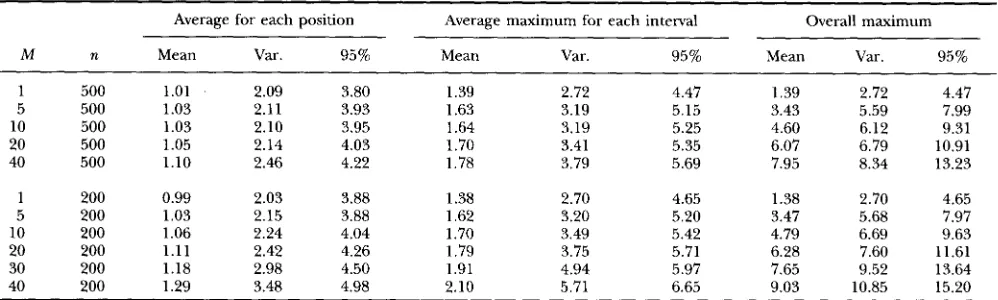
TABLE 2

Mean, variance (var.) and 95 percentile (95%) of the test statistics for a particular position, for a marker interval and for the whole genome under the null hypothesis

Average for each position Average maximum for each interval Overall maximum

M n Mean Var. 95% Mean Var. 95% Mean Var. 95%

1 500 1.01 2.09 3.80 1.39 4.47 1.39 2.72 4.47

5 500

2.72

1.03 2.11 3.93 1.63 3.19 5.15 3.43 5.59 7.99

10 500 1.03 2.10 3.95 3.19 5.25 4.60 6.12 9.31

20

1.64 500

40

1.05 500

2.14 4.03 1.70 3.41 5.35 6.07 6.79 10.91

1.10 2.46 4.22 1.78 3.79 5.69 7.95 8.34 13.23

1 200 0.99 2.03

5 200

3.88 1.38 2.70 4.65 1.38 2.70 4.65

1.03 2.15 3.88 1.62 3.20 5.20 3.47 5.68 7.97

10 200 1.06 2.24 4.04 1.70 3.49 5.42 4.79 6.69 9.63

20 200 1.11 2.42 4.26 1.79 3.75 5.71 6.28 7.60 11.61

30 200 1.18 2.98 4.50 1.91 4.94 5.97 7.65 9.52

40 200 1.29 3.48 4.98 2.10 5.71 6.65 9.03 10.85 15.20

13.64

All markers are linked on one chromosome with 10 cM for each marker interval. Replicates of simulations are 1000 for sample size n = 500 and 2000 for n = 200.

value of the test statistic for the test performed in a genome. To determine an appropriate critical value of the test statistic for this testing method, we need to know the behavior of the test statistic under the null hypothesis, not only for a particular interval, but for a whole genome, because the entire genome is tested for the presence of QTLs. LANDER and BOTSTEIN (1989) discussed the issue of the critical value of the test statistic (using the LOD score) for the simple interval mapping. The threshold of the test statistic for the composite interval mapping is, however, different. The difference is that with multiple regression the test statistic is more or less uncorrelated for different intervals [Property 41. Thus to achieve an overall significance level a for the test with M intervals, a nominal significance level a / M may be used for the test in each interval, a situation correspond- ing to the sparse-map case of LANDER and BOTSTEIN (1989).

However, the distribution of the maximum of LR over an interval ( i . e., the distribution of the LR of (13) taking

p

as a parameter) under the null hypothesis is not clear. This distribution will depend greatly on sample size, the number of markers fitted in the model and the genetic size of each interval. To investigate the behavior of the test statistic, a series of simulations were performed under the null hypothesis. Although our null hypothesis is that there is no QTL on the relevant interval being tested, no QTL in the genome was simulated to examine the behavior of the test statistic in a genome. This does not make much difference under our model because segregating QTLs on other intervals are more or less controlled by conditioning markers in the model so that they would not greatly influence the hypothesis testing on the interval being tested (cJ LANDER and BOTSTEIN 1989). Two extreme situations, linked and unlinked cases, were simulated. In the linked case, M equally spaced marker intervals (with M+1 markers) are located on one chromosome, and in the unlinked case, M

equally spaced marker intervals (with 2 M markers) are located on different chromosomes. For each replicate of simulations, n backcross individuals were simulated on M + l (or 2 M) markers (with the recombination frequency r for each marker interval) and a quantitative trait (simulated simply as a normal random variable). Analysis was performed as stated above, and LR test statistic was calculated by (13) along the genome at every l-cM position.

Results are presented in Table

2

and Figure 1. Table 2 gives the means, variances and 95 percentiles (over replicates) of LR for a particular position [ i. e., LR of (1 3) taking a fixed value for

$11,

the maximum of LR for a marker interval [Le., LR of (13) taking

p

as a parameter] and the overall maximum of LR over a genome under the null hypothesis. There is generally little difference among statistics of LR from position to position and from interval to interval, so only averaged statistics

(mean, variance and 95 percentile) of LR over all positions and over all marker intervals are presented. Fig- ure 1 plots the 95 percentiles of the overall maximum of LR against the number of intervals for sample sizes ( n )

500 and 200.

These results strongly suggest that, when the sample size is large and the number of markers fitted in the model is relatively small, the LR test statistic for f i x e d

testing position (i.e., for fixed

p )

is approximately distributed with 1 degree of freedom (with mean 1, variance 2 and 95 percentile 3.84), as might be expected [but see GOFFINET et al. (1992) for a special case]. When the sample size is relatively small and the number of markers fitted in the model is large, the observed LR deviates from

x:

distribution, most likely due to slow convergence of the statistic to

x:

distribution.

(7)

Mapping Quantitative Trait Loci 1463

A

B

o Linked, 10 c M v U n l i n k e d , 10 cM

Linked, 5 c M

6\0 16

In

2

-

_x

O.O5/Y,2

2 ~ i ' i ' i ' i i "

0 5 10 1.5 20 25 30 35 40 45 50

Number of i n t e r v a l s (M)

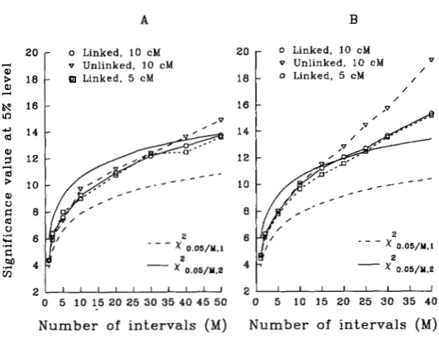
/ FIGURE 1.-The 95 percentile of the overall

maximum of the test statistic under the null hypothesis is plotted against the number of in- tervals ( M ) from simulation. Three cases are plotted. In the unlinked case, all marker in- tervals (with 10 cM) are on different chromo- somes. In the linked cases (one with a 10-cM interval and one with a 5-cM interval), all marker intervals are on one chromosome. The values of

x&,5,M,1

and

x:,05,M.2

are also plotted

X 0.05/&1 with 2000 replicates and 200 for graph B with

" _

2 for reference. Sample size is 500 for graph A

2 5000 replicates.

0 5 10 15 20 25 30 35 40

N u m b e r of i n t e r v a l s

(Ma>

M = 30 and

40

in which the number of degrees of freedom for the test is reduced significantly). The distribution depends on the sample size, the number of markers fitted in the model and the genetic size of the interval. The correlations of maxima of LRs between intervals are generally very small (positive) [Property 41. (The average correlations for adjacent intervals are generally less than 0.3 and the average correlations for non-adjacent intervals are effectively close to zero.) The effect of marker interval size (comparing the cases of lOcM interval with 5-cM interval in Figure 1) tends to be minor, compared with other factors such as sample size, number of markers fitted in the model and number of intervals tested. Thus it appears that when the sample size is large and the number of markers fitted in the model is not too many,

x : , ~ , ~

can be used as an approximation for the lOOa% critical value for an overall test with M intervals in a genome for the model (5) (Figure 1A). (Although only the 5% critical value is presented in Figure 1, other critical values such as 10% show similar patterns.)

However, in practice, sample sizes of mapping data are generally not very large, and markers are unlikely to be evenly spaced in the genome. In that case, it may not be appropriate and desirable to fit too many markers in the model even when they are unlinked to the interval being tested, because too many markers fitted in the model can substantially increase the critical value of the test statistic [for example, comparing the cases of linked ( M

+

1) markers with unlinked ( 2 M ) markers in Figure lB] , and thus reduce the power of the test. Many markers in mapping data are also usually clustered in some regions. If that is the case, it would be more appropriate to use in the model as a control only those selected markers which are more or less evenly spaced in the genome or those preidentified markers ( e . g . , by stepwise regres-

sion) which explain most of the genetic variation in the genome. Other markers can still be used for testing QTLs at relevant intervals. For many data, the above criterion may be used as a guide (not necessarily for

a = 0.05). If necessary, computer simulations can be used to determine an appropriate critical value for the test for a given data set.

QTL MAPPING SIMULATION ANALISIS

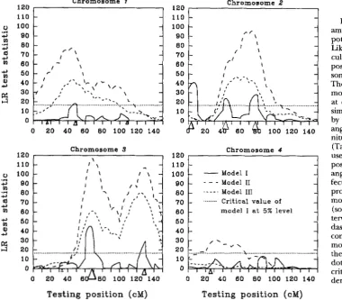
Methods: To illustrate the properties, utility, advantages and disadvantages of the method, a simulation study of mapping QTLs was performed. Four "chromosomes" each with 16 markers separated in 15 10-cM intervals were simulated for a backcross population. The trait is affected by 10 QTLs with positions and effects given in Table 3 and depicted in Figure

2.

Together the QTLs account for

70%

of the phenotypic variance in a backcross population. Sample size is 300. The trait value of an individual is determined by the sum of effects of the QTLs which the individual possesses, plus a random

(environmental) variable which is normally distributed with mean zero and variance scaled to give the expected 0.7 heritability of the population. Both marker and QTL types were simulated for each individual with the linkage map specified above.

This data set can be fitted for analysis by numerous models. For the purpose of illustration, three simplified models were fitted in the analysis following the procedures outlined above:

Model I: Composite interval mapping with k in model (5) summed over all other markers (solid curves of Figure 2 ) ;

Model 11: Semi-composite interval mapping with k

(8)

1464 Z.-B. Zeng

TABLE 3

Parameters and point estimates of positions and effects of QTIS from one replicate of simulation

~

Chromosome I Chromosome 2 Chromosome 3 Chromosome 4

Position (cM): 16 48 108 3 43 77 33

0.42

68

Effect: 0.75 129 26

Parameters

0.58 1.02 -1.23 -1.26 -0.46 1.61 0.88 0.74

~~

Model I

Position (cM) 48

Effect 1.02

Position (cM) 45

Effect 1.18

Position (cM) 45

Effect 1.42

Model I1

Model 111

Point estimates

6 43 78 66 130

1.29 -1.16 -1.18 1.68 1.39

73 -1.43

65 -1.46

68 130 32

1.67 1.52 0.69

69 125

1.60 1.83

Point estimates of QTL effects are made at the peaks of the likelihood profile in the regions where the presence of QTLs is indicated (see Figure 2).

Chromosome 1

0 100

.d 4

VI

4

tu

.d

4 m

4

Q VI

4

5

30 “, ...

0

-.

0 20 40 80 80 100 120 140

120

,

Chromosome 3 _I

110

-

I \ \

-

I \ \

--.

0 100

-

I \

.-I

I \

-

4 90

‘ I

VI

-

/ ‘

\

I

-60

-

Testing position (cM)

50 40 30 20 10 0

100 120 140

120 110 100

-

- -

Model I 9 0 - - - - Model I1

80

-

Model I11

-

7 0

-

... Critical value of

-

60

-

50

-

model I a t 5% level -

-

/ -

30

-

40

Chromosome 4

-

I ” d \

20 _:=..= ... ... I

0 20 40 6 0 80 100 120 140

Testing position

(cM)

Model 111: Simple interval mapping with model (3) (short-dashed curves of Figure 2).

The dotted lines of Figure 2 give the simulated overall 5% critical value, 16.5, for the test of model I (based on a simulation with 5000 replicates under the null hypoth-

esis), which is a little higher than

x:,05,60,2

-

x

~

,

-

~

,

~

14.2. The overall 5% critical values for models I1 and I11 are smaller (12.6 for model I1 and 10.7 for model 111). Some point estimates of positions and effects of QTLs at

- 2 -

FIGURE 2.-A simulation example of QTL mapping on an hy- pothetical backcross population. Likelihood ratio test statistic is calculated and plotted at every 1 c M position of the four “chromosomes” to give a likelihood profile. The genetic length of each “chromosome” is 150 cM with markers at every 10 cM. Ten QTLs were simulated with positions indicated by triangles. The size of each tri- angle is in proportion to the mag- nitude of the effect of the QTL (Table 3). Dark-sided triangles are used to indicate for QTLs with positive effects, and light sided tri-

angles for QTLs with negative effects. Three curves (likelihood profiles) are plotted for the three models fitted for analysis: model I (solid curves) is the composite interval mapping, model I1 (long- dashed curves) is the semi- composite interval mapping and model I11 (shortdashed curves) is the simple interval mapping. The dotted line is the simulated 5% critical value, 16.5, for the test under model I.

the peaks of the likelihood profile in the regions where the presence of QTLs is indicated are given in Table 3 for reference. Both Figure 2 and Table 3 depict results of mapping of a single replicate of simulation.

(9)

s

d

.I

cl II 8

i

!?

1 0

2

rcr

f

8

6

0, rcr

e

* a

d B

$

:f!

71

H 8_a

rcr

.!

h:

II

*n 8 *%

2 !i-

a

I

U

E

3

&

I

-$.

B

s!

e

w o

E"

_r:

_"

8

m

W a 0 ET c9 3 R\

E"

3

0

% -

5

E

e

c (D COO n l 1 W c" f - I

o'!

C u e

9

$ g

E , & 5 2 c-7

8

S T

"

ET

n - 9

m q GQO 0 H .1

;

e

8 "

coo

i

_m

r: 1 ET

2 0

8

Y

8 ,

73 u

'R e,

a w O b

Mapping Quanti1

"wm hc-7

_^I

"9"lI? 1"

S Z Z Z 2% 5%

-e h

r- m m c n ~ m w

1-!Sr:? ?Or- "F?

of-r-0- or-0 O b 0

ETm ET m

?"e?

DVCZO_

"n " a

~~

w "LC

0 0 0 0 3

q?oS-! n n 3 - "

0 2

;g

o m ,

?Lo.?

2

"3 " Ss:

eo,

99m! 0 . 0 "

3 3 1 3

m

"

" ? ? " ? ?

22

"(De A n h

EZSZ S Z "

-sl

$c?qg%

& $

e??

2

O W W " 3 0 3

w w r-

T I

%I

2

L1

8 -

_E

-3

Y)

'5

'3

B

5 $

rn I I I I

h h m 0

S W ? "

E5Z.S

"

0 "ET

$ Z $ Z ?

fir- I I

"mi r"

1 9 " " ZZZZ

"

n * a

" *

I I

%?rr

""

0

S I ? ? GESS

c9-??99

A h

f- 0.100

OCOC03-l

-In

?I

SZ

h

o f -

? S F

1 3 -

f - l

-

2 :

.s

2 3 2

SZ

2

4

'B

.e

-s

y

5 9 s

%

;

$ 2

c

p a d

g

$ 3

m z 3

5 z

0

E

3

P - 1 a

.g

3"

'cl

e 2

$ 0 a

$ 2

E

2 3 3

,232

z

t i 8 z

e

.z

'3

z;;

S ? vi

.- e c

c o o

2 3 2 5 h 3 c o = a

u"

" " - h

m W V 0 rr) 0 0 U m m

m .

& - -

2 5 5 . G C

o m o o - - 0 -

" a m

I?"? T& Ys:

"'49rnri 9°C

2 x 2

Y) w 0

ZSSO_

ce-

co,

8 h 3 c

5 2 ;

* m

"

m

.;la= b .9 .5

a.;

.s

5

'g

'6

"

Z C G

o l d t i

% a = w

2 X - E

88

8

Q

gz<

5 '$2;

-

0 L .o c e ocL1*, 3 $?d

2%

$?-

a 6

9

3 g'g'g&&%

e, 3'3

3 z"&:z

o

g & 3

u

g:;g

.;

6 6

O & & C k c r l W 0 B&LW O & & W

& g

9 u 9

h

" v

-

",a=

E

E 8

E 0 - u

ative Trait Loci 1465

of QTLs which are indicated in Figure 2 are reported. For each replicate, estimates were made at the distinctive peaks of the likelihood profile around the relevant regions. Although Figure

2

is an analysis based on a single replicate, the general patterns of mapping among 100 replicates conform to that of Figure

2.

There are, however, a few replicates for which the mapping under models I1 and 111 indicates only one rather than two QTLs on "chromosome" 3. In these cases, to make the results comparable with other replicates, the results were still interpreted to indicate two QTLs and estimates of positions and effects of QTLs were made at relevant local maxima of the likelihood profile. Empirical estimates of the power of the test

(i.

e., the ratio of the replicates that are significant at the relevant regions over the total r e p licates) are also presented in Table

4.

Results: In this analysis, neither model

I1

nor model 111 controls the effects of possible QTLs located at other regions of the chromosome when testing for a QTL at a particular chromosome position. Model 11, however, effectively removes, from the residual variance of the model, most of the variation due to segregating QTLs located on unlinked chromosomes, so that the LR test statistic on most intervals under this model is significantly larger than those under the other two models

[Property 21. This model has the highest statistical power, among the three models, for detecting marker and QTL linkages. However, as the test under model

I1

(as well as model 111) is not an interval test, this model does not necessarily have high probability of locating individual QTLs accurately, because estimates of position and effect of a QTL can be influenced by other linked QTLs. Only model I provides an interval test in which the test statistic on an interval is unaffected by all those QTLs which are located outside the interval being tested and its two adjacent intervals. This is an advantage of the interval test. Model I also effectively removes from the model residual variance most of the variation due to segregating QTLs. However, because the test under model

I

is a conditional test [Property 3, see ZENC (1993) for more detailed discussion on the theoretical ground], the test statistic on many intervals is smaller than those under models

I1

and I11 (Figure

2).

This is a disadvantage of the interval test.

Nevertheless model I correctly identifies the six larg- est QTLs with relatively higher resolution in Figure

2,

judged by the relatively accurate positions of the significant peaks of the likelihood profile and also by the slope of the likelihood profile (see also Table 4). This increase of precision of mapping is gained by making the test conditional on nearby markers so that the sensitivity of the test statistic to the position of a QTL is increased and the position effect of a QTL is emphasized in a short region of the interval conditioned. This is another advantage of the interval test.

(10)

1466 Z.-B. Zeng

correctly indicate the presence of two major QTLs (the third QTL is minor), because the two QTLs are separated by a sufficiently long distance. On “chromosome” 2, however, the likelihood profiles of models I1 and 111 seem to indicate the presence of a single QTL at wrong positions. This is due to the presence of three QTLswith comparable (and opposite) effects in a relatively close range. Should this occur, we could be deceived by using wrong models. Of course, these data can be fitted and analyzed for two or three QTLs simultaneously as suggested by LANDER and BOTSTEIN (1989), but the statistical tests for two QTLs us. one QTL, and three QTLs us. two QTLs are not easy matters. In real applications, the number of QTLs on a chromosome ( i e . , the true genetic model for testing) is unknown, and we can very easily be deceived by fitting and testing the wrong models. Also, even when the correct region of a QTL can be identified under models I1 and 111, the likelihood profiles under models I1 and 111 tend to be flatter ( i. e . , the supporting intervals as defined by LANDER and BOTSTEIN (1989) are wider) (Figure

2)

and the precision of mapping is still relatively lower (Table 4).

It seems that only model I is more likely to give unbiased estimates of position and effect of QTLs (Table 4 ) . However, as discussed above, model

I1

has the highest statistical power for identifjmg possible QTL regions, and the statistical power of model I for identifying QTLs is relatively lower (and can be very low), because of the fitting of the closely linked markers in the model [Prop- erty 31. Only model I1 strongly indicates the presence of a QTL on “chromosome” 4 in Figure

2.

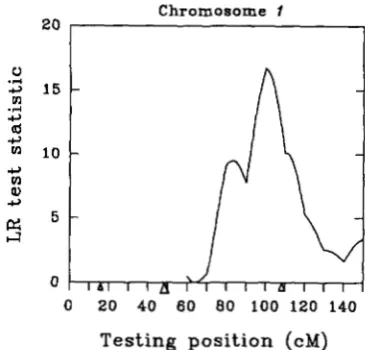
In practice, with limited data, some combinations of models I and I1 (2. e . ,

deleting or inserting some linked markers as a control in the model) may have to be used to maximize the probability of detecting QTLs while controlling the precision of mapping ( i . e . , balancing the type I and type I1 errors of the statistical test). This is illustrated, as an example, by a further analysis on “chromosome” 1 of the simulation example given in Figure 2. On this chromosome, both models I1 and I11 give a major peak of the likelihood profile in Figure

2,

which would indicate the presence of a QTL somewhere on the fifth interval. How- ever, model I1 also seems to suggest a second QTL roughly located between positions 70 and 110 cM for which the test under model I failed to show significance. To test this hypothesis, a test can be performed between 60 and 150 cM using a model combining model I1 with six more markers located between 0 and 50 cM for background control. This would eliminate the effect of the QTL mapped on the fifth interval (and also other possible QTLs on the left of 50 cM position) in the test and estimation. Indeed this test strongly indicates the presence of another QTL with effect estimated to be 0.52 at position 100 cM (Figure 3 ) .

On the accuracy of estimates of QTL effects, we have to distinguish two issues affecting the relative accuracy

20

I

Chromosome 1

0 2 0 40 6 0 8 0 100 120 140

Testing position (cM)

FIGURE 3.-A reanalysis of Figure 2 for mapping for a QTL on the region between 60 and 150 cM of “chromosome” 1 . The test for a QTL at each position is conditional on fitting 6 markers located between 0 and 50 cM of “chromosome” 1 and all other unlinked markers. There is strong evidence for the pres ence of one more QTL on this chromosome by this analysis. The effect of the QTL is estimated to be 0.52 at position 100 cM.

of estimates: bias and sampling error. Estimates of QTL effects under model I tend to be less biased compared with those under models I1 and 111, because the estimates under model I are unaffected by QTLs that are located at other marker intervals [Property 11 (Table 4). However, the estimates under model I will have larger sampling variance than those under model I1 [Property 31 (Table 4). If we know that there is at most one QTL on a chromosome, model I1 tends to have both higher statistical power for the test of QTL and smaller sampling variance for the estimate of QTL effect (see, for example, chromosome 4 of Table 4); otherwise the test and estimation under model I1 (and also model 111) can be misleading and QTLs can be mapped to wrong

po-

sitions (or intervals).

(11)

Mapping Quantitative Trait Loci 1467

the sampling variance of estimates particularly when the sample size is small. In practice, we may need first to select a few markers for each chromosome or some chro: mosomes by, for example, stepwise regression and use those markers to control genetic background when mapping QTLs by interval test.

DISCUSSION

For mapping QTLs, unbiasedness and accuracy should be more important than other issues of mapping techniques, such as ease of computation. Because quantitative trait variation is generally influenced by multiple genes, we have to take into account effects of possible multiple (linked) genes when designing a mapping method. Effective control of individual gene effects is a key to increasing the precision of mapping. Every effort should be made in mapping to preserve the accuracy and quality of mapping and at the same time to maximize the chance of finding more QTLs.

A new QTL mapping framework is proposed in this paper. The key feature of the approach is the idea of an interval test which tries to separate and isolate individual QTL effects when testing and mapping for QTLs. De- pending on data and underlying genetic mechanisms, the precision of mapping can be significantly improved. The method works better for traits with high heritability, because most of the genetic variation can be controlled and removed from the residual variation in the model by conditioning on multiple markers. For traits with low heritability, the gain of fitting multiple markers in the model as a control may not justify the cost in losing statistical power of finding a QTL due to both increased sampling variation of estimates if closely linked markers are fitted in the model for an interval test [Property 31, which would reduce the test statistic, and increased threshold of the test (this is due to both increased number of intervals tested and reduction of degrees of freedom of the test). In that case, the first task might be to increase the chance of finding anything in the genome. In practice, the best strategy would be to fit data with multiple models to identify an appropriate model which balances both type I and type I1 errors of the test.

In this study, only the backcross population design is analyzed. Other population designs, such as F, populations, and dominant genetic models can readily be implemented in this framework, Epistasis is, however, ignored here. With possible epistatic effects of QTLs, this mapping method can still be biased. Problems with analyzing epistatic effects of genes in mapping QTLs are that there could be many types of genetic epistasis and that the underlying genetic parameters for epistasis are not well defined. In principle, epistatic effects can be fitted in the model for mapping QTLs if the type of genetic epistasis is identifiable ( e . g . , HAL,EY and

mom

1992).

Regression analyses have been used for mapping

QTLs in various ways by HALEY and KNOTT (1992), MAR-

TINEZ and CURNOW (1992), MORENO-GONZALEZ (1992),

andJANSEN (1992,1993). Both HALEYand ~ O T T (1992)

and MARTINEZ and CURNOW (192) used the regression

analysis simply to approximate the simple interval mapping procedures, although they also suggested using a bivariate regression analysis to search the two- dimensional space along the chromosome for mapping two QTLs. MORENO-GONZALEZ (1992) proposed a step wise multiple regression procedure to fit multiple markers (with multiple “QTLs” arbitrarily assumed to be located in the middle of each marker interval) in the model for mapping QTLs. It appears that this procedure is very arbitrary and imprecise.JANsEN (1992) described a mixture model analysis in the framework of the interval mapping. He, however, gave a simulation example of using a third marker as a covariable in the linear model as a control, which has some similarity to the method proposed here. Very recently, JANSEN (1993) also pro-

posed a procedure for mapping QTLs which combines interval mapping with multiple regression. There are some similarities between the method of ZENC (1993)

(and also here) and that ofJANsEN (1993). But clearly, there are critical differences in concepts and procedures to map multiple linked QTLs. The method used in this paper is the interval test. The emphasis is to control the precision of mapping as much as possible. JANSEN (1993), however, used a procedure of testing multiple markers on a chromosome simultaneously to indicate possible multiple QTLs on a chromosome, which seems to be very imprecise for mapping multiple QTLs. More- over, many theoretical and statistical properties and be- haviors of their method were not analyzed and discussed

by JANSEN ( 1993).

(12)

1468 Z.-B. Zeng

control the residual genetic variation in the rest of the genome for the test (interval test).

BRUCE WEIR, C. CLARK COCKERHAM, BILL HILL, REBECCA DOERGE and DENNIS Boos provided constructive comments on the manuscript.JoHN MONAHAM provided constructive advice on computational implemen- tation. This study is supported in part by grants GM 45344 from the National Institutes of Health and DEE9220856 from the National Sci- ence Foundation.

LITERATURE CITED

COWEN, N. M., 1989 Multiple linear regression analysis of RFLP data sets used in mapping QTLs, pp. 113-116 in Development and Ap- plication of Molecular Markers to Problems in Plant Genetics,

edited by T. HELENTJARIS and B. BURR. Cold Spring Harbor Labo- ratory, Cold Spring Harbor, N.Y.

GOFFINET, B., P. LOISEL and B. LAWRENT B., 1992 Testing in normal mixture models when the proportions are known. Biometrika 79:

HALEY, C. S., and S. A. &om, 1992 A simple regression method for mapping quantitative trait loci in line crosses using flanking markers. Heredity 6 9 315-324.

HILBERT, P., K. LINDPAINTER, J. S. BECKMANN, T. SERIKAWA, F. SOUBRIER, C. DUBAY, P. CARTWRIGHT, B. DE GOWON, C. JULIE, S. TAKAHASI, M. VINCENT, D. GANTEN, M. GEORGES and G. M. LATHROP, 1991 Chro- mosomal mapping of two genetic loci associated with blood- presume regulation in hereditary hypertensive rats. Nature 353:

JACOB, H. J., K. LINDPAINTER, S. E. LINCOLN, K. KUSUMI, R. K. BUNKER, Y.-P. mo, D. GANTEN, V. J. DZAU and E. S. LANDER, 1991 Genetic m a p ping of a gene causing hypertension in the stroke-prone rat. Cell 67: 213-224.

JANSEN, R. C., 1992 A general mixture model for mapping quantitative trait loci by using molecular markers. Theor. Appl. Genet.

JANSEN, R. C., 1993 Interval mapping of multiple quantitative trait loci. Genetics 135: 205-211.

KNAPP, S. J., W. C. BRIDGES, JR., and D. BIRKES, 1990 Mapping quantitative trait loci using molecular marker linkage maps. Theor. Appl. Genet. 79: 583-592.

KNOT, S. A,, and C. S. HALEY, 1992 Aspects of maximum likelihood methods for the mapping of quantitative trait loci in line crosses. Genet. Res. 6 0 139-151.

LANDER, E. S., and D. BOTSTEIN, 1989 Mapping Mendelian factors

842-846.

521-529.

8 5 252-260.

underlying quantitative traits using RFLP linkage maps. Genetics 121: 185-199.

MARTINEZ, O., and R. N. Cumow, 1992 Estimation the locations and the sizes of the effects of quantitative trait loci using flanking markers. Theor. Appl. Genet. 85 480-488.

MENG, X.-L., and D. B. RUBIN, 1993 Maximum likelihood estimation via the ECM algorithm: a general framework. Biometrika 8 0

MCLACHLAN, G. J., and K. E. BASFORD, 1988 Mixture Models: Inference

and Applications to Clustering. Marcel Dekker, New York. MORENO-GONZAWZ, J., 1992 Genetic models to estimate additive and

non-additive effects of marker-associated QTL using multiple regression techniques. Theor. Appl. Genet. 85: 435-444.

PATERSON, A. H., E. S. LANDER, J. D. HEWIIT, S. PETERSON, S. E. LINCOLN and S. D. TANKSLEY, 1988 Resolution of quantitative traits into Mendelian factors by using a complete RFLP linkage map. Nature

PATERSON, A. H., S. DAMON, J. D. HEWIIT, D. ZAMIR, H. D. RABINOWITCH, S. E. LINCOLN, E. S. LANDER and S. D. TANICSLEY, 1991 Mendelian

factors underlying quantitative traits in tomato: comparison across species, generations and environments. Genetics 127: 181- 197.

RODOLPHE, F., and M. LEFORT, 1993 A multi-marker model for detecting chromosomal segments displaying QTL activity. Genetics

STAM, P., 1991 Some aspects of QTL analysis, in Proceedings of the Eighth Meeting of the Eucarpia Section Biometrics in Plant Breed- ing. Brno, July 1991.

SOLLER, M., T. BRODY and A. GENIZI, 1976 On the power of experimental design for the detection of linkage between marker loci and quantitative loci in crosses between inbred lines. Theor. Appl. Genet. 47: 35-39.

STUBER, C. W., S. E. LINCOLN, D. W. Worn, T. HELENTJARIS and E. S. LANDER, 1992 Identification of genetic factors contributing to heterosis in a hybrid from two elite maize inbred lines using molecular markers. Genetics 1 3 2 823-839.

TITTERINGTON, D. M., A. F. M. SMITH and U. E. m o v , 1985 Statistical

Analysis of Finite Mixture Distributions. Wiley, New York. WELLER, J. I., 1986 Maximum likelihood techniques for the mapping

and analysis of quantitative trait loci with the aid of genetic markers. Biometrics 42: 627-640.

ZENG, Z.-B., 1993 Theoretical basis of separation of multiple linked gene effects on mapping quantitative trait loci. Proc. Natl. Acad. Sci. USA 90: 10972-10976.

267-268.

3 3 5 721-726.

134: 1277-1288.