Shielded Source Analysis using Precalculated Library Estimates.

(1)

ABSTRACT

HOLMES, THOMAS WESLEY. Shielded Source Analysis using Precalculated Library Estimates. (Under the direction of Robin Gardner.)

(2)

c

(3)

Shielded Source Analysis using Precalculated Library Estimates

by

Thomas Wesley Holmes

A thesis submitted to the Graduate Faculty of North Carolina State University

in partial fulfillment of the requirements for the Degree of

Master of Science

Nuclear Engineering

Raleigh, North Carolina

2013

APPROVED BY:

John Mattingly David Lalush

Dean Mitchell Robin Gardner

(4)

BIOGRAPHY

Thomas Wesley Holmes was born in Raleigh, NC on the 31st _{of October, 1986. He received}

(5)

ACKNOWLEDGEMENTS

I would like to thank my advisor for his help, my family for their unwavering love and support and my friends for some much needed relief. Also, Sara, my favorite, thank you.

(6)

LIST OF TABLES

Table 2.1 Dimensions of the Shielding Materials . . . 11

Table 2.2 Thicknesses of the Shielding Materials . . . 12

Table 3.1 Sources with their associated centroids and associated FWHM in MeV 16 Table 5.1 Thicknesses of the Test Spectrum for the First Data Set in Centimeters 36 Table 5.2 Thicknesses of the Test Spectrum for the Second Data Set in Cen-timeters . . . 38

Table 6.1 Upper Limit Cutoff Values and their Energies for Each Radioisotope 45 Table 6.2 Thicknesses of the Test Spectrum for the First Data Set in Centimeters 48 Table 6.3 Averages of 30 Trials with the First Data Set Using137_{Cs . . . . .} ₅₁

Table 6.4 Averages of 30 Trials with the First Data Set Using60_{Co . . . .} ₅₂

Table 6.5 Averages of 30 Trials with the First Data Set Using238_{U . . . .} ₅₃

Table 6.6 Averages of 30 Trials with the Second Data Set Using 137_{Cs . . . .} ₅₅

Table 6.7 Averages of 30 Trials with the Second Data Set Using 137_{Cs Over a} Reduced Range . . . 57

Table 6.8 Averages of 30 Trials with the Second Data Set Using 60_{Co Over} the Full Range . . . 59

Table 6.9 Averages of 30 Trials with the Second Data Set Using 238_{U Over a} Limited Range . . . 61

Table 8.1 Preliminary Correlations to the Unknown Input Spectrum . . . 74

Table 8.2 Initial Guesses for Each Sector . . . 75

Table 8.3 Correlations from Each Interpolated Sector . . . 76

Table 8.4 Slope, Y-Intercept and Sum of Squares Statistics for Each Sector . 76 Table 8.5 Final Choices before Sector Selection . . . 77

Table 8.6 Final Answer . . . 77

Table 8.7 First Data Set Library Using137_{Cs with Automatic Guesses Generated 79} Table 8.8 First Data Set Library Using60_{Co with Automatic Guesses Generated 81} Table 8.9 First Data Set Library Using238_{U with Automatic Guesses Generated 82} Table 8.10 Second Data Set Library Using137_{Cs with Automatic Guesses} Gen-erated . . . 84

Table 8.11 Second Data Set Library Using 60_{Co with Automatic Guesses} Gen-erated . . . 86

Table 8.12 Second Data Set Library Using 238_{U with Automatic Guesses} Gen-erated . . . 87

(8)

LIST OF FIGURES

Figure 1.1 Side views of the 1D configuration and the 3D configuration re-spectively. . . 4 Figure 1.2 Comparison of the detector outputs from the 1D and 3D simulations. 5 Figure 2.1 A crossectional view (diagram) of the benchmark configuration

with all materials in the standard position. . . 8

Figure 3.1 Natural Log of Centroids V.S. FWHM and its Linear Trend . . . 15 Figure 3.2 Data Set from ’mmm’ to ’ppp’ Configurations using 137_{Cs . . . . .} ₁₈ Figure 3.3 Peak Normalized Data Set from mmm to ppp Configurations using

137_{Cs . . . .} ₁₉ Figure 3.4 Data Set from null to sss Configurations using 137_{Cs . . . .} ₂₀ Figure 3.5 Peak Normalized Data Set from null to sss Configurations using137_{Cs 21} Figure 3.6 Set from mmm to ppp Configurations using 60_{Co . . . .} ₂₂ Figure 3.7 Peak Normalized Data Set from mmm to ppp Configurations using

60_{Co . . . .} ₂₃ Figure 3.8 Data Set from null to sss Configurations using 60_{Co . . . .} ₂₄ Figure 3.9 Normalized Data Set from null to sss Configurations using 60_{Co .} ₂₅ Figure 3.10 Data Set from mmm to ppp Configurations using 238_{U . . . .} ₂₆ Figure 3.11 Peak Normalized Data Set from mmm to ppp Configurations using

238_{U . . . .} ₂₇ Figure 3.12 Data Set from null to sss Configurations using 238_{U . . . .} ₂₈ Figure 3.13 Peak Normalized Data Set from null to sss Configurations using 238_{U 29} Figure 4.1 Tri-linear Interpolation Method . . . 31 Figure 4.2 Physical Interpretation of the Shielding Materials for Tri-linear

In-terpolation . . . 33 Figure 5.1 Peak Normalized Unknown Test Spectra for the First Data Set

Using137_{Cs . . . .} ₃₇ Figure 5.2 Peak Normalized Unknown Test Spectra for the First Data Set

Using60_{Co . . . .} ₃₉ Figure 5.3 Peak Normalized Unknown Test Spectra for the First Data Set

Using238_{U . . . .} ₄₀ Figure 5.4 Peak Normalized Unknown Test Spectra for the Second Data Set

Using137_{Cs . . . .} ₄₁ Figure 5.5 Peak Normalized Unknown Test Spectra for the Second Data Set

(9)

Figure 5.6 Peak Normalized Unknown Test Spectra for the Second Data Set Using238_{U . . . .} ₄₃ Figure 6.1 Interpretation of the Sector for Unknown 1 in the First Data Set . 46 Figure 6.2 Tri-Linear Fit for the 30th _{Trial in Table 6.2 . . . .} ₄₉

Figure 7.1 Peaks VS FWHM and the 2n_d _{Order Power Series Fit . . . .} ₆₇

Figure 8.1 Linear Stripping and Shielding Material Presence Determination . 73

(10)

Chapter 1 Introduction

In many common real world situations, analysis of gamma spectra is needed in circum-stances that contain unknown shielding materials with an associated unknown thickness that includes an unknown source and strength. This problem becomes more complicated when there are perturbations in the known background that stem from an array of un-foreseeable circumstances. The long list of unknown parameters causes the pathway for any solution to require a variety of techniques for determining these factors.

In this discussion, the main focus will be placed on the situation of a shipping cargo container but the overall approach can be applied to a variety of problems. Cargo con-tainers are of special importance because a common fear when dealing with incoming cargo containers, both domestic and international, is the threat of clandestine nuclear materials. With this possibility in mind, it would only make logical sense to use the most accurate tools available for more precisely assessing the potential presence of malicious nuclear materials within any container.

(11)

intensity and the shielding materials at hand. Several approaches for determining the various radionuclides within any given spectrum have implemented the method of least squares analysis. Salmon was a primary contributor to this approach in 1961 where he established its ability to successfully determine the composition and contribution of a spectrum with six separate sources and their associated spectra. He was able to complete this task by recognizing that the Compton continuum of the higher energy photo peaks impacted the shape of the lower energy peaks. To account for this, he used the entire spectrum of all of the radioisotopes found within the spectrum in his calculations. This successful demonstration of the least squares approach has lead to similar techniques that have been applied previously at NC State University for the measurement applications of prompt gamma-ray neutron activation analysis and x-ray fluorescence spectroscopy for elemental analysis (Guo, Gardner).

In order to first determine which radioisotopes are present in a given spectrum, the simplest approach is to identify each full energy peak. Based on these full energy peaks and their relative intensity, corresponding radioisotope signature patterns can be found. The basic count rates over these full energy peaks can be attributed to the relative activity concentration after background has been subtracted from the spectrum. This type of spectral deconvolution is performed using knowledge of the signature spectral response of the types of sources that should and could be present within the given situation. Spectral stripping is known as the peeling away each radionuclide spectral component from the original spectrum over the entire energy space starting from the highest energy and moving downward. As noted by Allyson, the use of the stripping technique is limited in its ability to represent artificial scattering of the source particles interacting with materials before being collected.

There is a fundamental issue when attempting to resolve these various unknown

(12)

shielding materials and their associated unknown thicknesses when given a spectrum of an unknown source and activity, which is centered on the idea that the peak value does not contain all of this information. The principal means by which to identify a source is by its high intensity photo-peaks but in the situation that there is little to no knowledge of several shielding materials and the initial source strength, a complex density transmission gage using these photo-peaks is not possible after source identification. The most appropriate means to determine the shielding material is to consider the portion of the spectrum that has interacted with the material, scattered and then been collected by the detector. Due to the range of incident energies considered in this application the region that needs to be considered for shielding material identification is from incoherent scattering events which are dominated by Compton scattering that reside below the full energy photo-peak.

(13)

to detector, where each case contained the same thickness of each but the shape of the shielding materials varied between the two scenarios. The 1D case consisted of three concentric spheres and the 3D case consisted of the first two shielding materials (lead and aluminum) as right circular cylindrical cans and the outer most shield of wood in the shape of a square box. The geometric description of each can be found in figures 1 and their corresponding detector outputs are given in figure 2. The source used in these simulations was137Cs which was placed in the center of the system and a 2 X 4 X 16 box style NaI(Tl) detector was placed 75 cm from the source with the 4 X 16 side facing the system.

Figure 1.1: Side views of the 1D configuration and the 3D configuration respectively.

Within the simulated detector responses (Gardner, 2004), there was a noticeable difference along the Compton continuum which was directly related to the geometric

(14)

1·10-5 1·10-4

0 0.1 0.2 0.3 0.4 0.5 0.6 0.7 0.8

N

ormalized Counts

Energy Bin [MeV]

1D 3D

1·10-1 1·100

0 0.1 0.2 0.3 0.4 0.5 0.6 0.7 0.8

Pe

ak-Normalized Counts

Energy Bin [MeV]

Figure 1.2: Comparison of the detector outputs from the 1D and 3D simulations.

(15)

Chapter 2 MCLLS and Library Setup

The primary tool used in this evaluation of the differences in shielding materials employs the Monte Carlo Library Least Squares (MCLLS) method. This approach uses a series of libraries based on very accurate pre-calculated forward models to fit an unknown data set which in this case is a spectrum (Gardner, Sood, 97). This method is very useful in evaluating inverse spectral problems and while it may require more effort than peak transmission gauges, it is more advantageous in that it uses the entire spectral data available and generates better accuracy of its solution (Metwally). This technique has proven itself to be successful for the inverse elemental analysis of prompt gamma-ray neutron activation analysis and energy-dispersive X-ray fluorescence analyzers (Gardner, Sood, 04).

As a means to use the MCLLS process, a generalized FORTRAN code has been de-veloped by Gardner for determining the parameters of a fitting model for a given data set. This package has been called CURMOD, which is based on the CURFIT subroutine developed by Bevington, and has served as the backbone for many specialized code devel-opments. CURMOD can be used to describe a data set using any combination of linear

(16)

and non-linear parameters. Accurate guesses are required for each non-linear parameter but they are not required for the linear parameters. CURMOD uses the Levenberg-Marquardt non-linear search method for finding a solution to the non-linear parameters and a multiple linear regression in determination of the linear parameters. It uses a min-imized reduced χ2 _{found in the following equation to select the best fit for all of the} parameter values.

χ2_red = χ 2

ν =

1

ν

X₍O−E)2

σ2 (2.1)

Where ν is the number of degrees of freedom,σ2 is the variance of the observation, O is the observed data and E is the theoretical data. Also CURMOD quantifies the error associated with each parameter for the final fit to the input data set.

Given the problem at hand, where there is a combination of unknown shielding mate-rials along with an unknown radionuclide and source strength, the linear and non-linear parameters must be reduced to produce a generalized situation that can be resolved. These simplifications were based around the operating conditions for the primary de-vices currently used for cargo monitoring that are probably akin to the nightmares of those that dream of precise and stable laboratory measurements. The contents of the sample (or cargo container) are usually of largely unknown composition and geometry. If illicit radioactive materials are intentionally present, they are likely to be concealed using unknown shielding materials and in many cases it is not feasible to perfectly control the speed and positioning of the container passing through the monitor.

(17)

are variable amounts of unknown shielding, with a distance on the order of meters between the source and detector. The scheme depicted in the following figure is a cross sectional view of what was developed with these characteristics in mind.

Figure 2.1: A crossectional view (diagram) of the benchmark configuration with all materials in the standard position.

This design included three different shielding materials of lead, aluminum and wood with each having three equally thick shielding components and a null condition where the material is entirely removed. The inner two materials were in the shape of a right cylindrical cans and the outer most shielding material was in the shape of a cube. The

(18)

detector used was a 2 X 4 X 16 box style NaI(Tl) detector that was placed one meter from the point source located in the center of the system.

The idea of using multiple shielding materials to determine the composition of any absorbing material was first conceptualized by Estep and Sapp. This approach was called the material basis set method and was based on the effective atomic number principle. This principle considered that the attenuation properties of gamma rays though any element could be closely approximated by a combination of basis materials mixed in the appropriate proportions. It was proposed that in most applications, two materials were sufficient in producing an equivalent attenuation map but this idea was expanded upon in this specific application by adding a third member to the basis materials and adding multiple thicknesses of these materials. This improvement was selected to gain added accuracy to the final result, allow for a larger range of possibilities and span a wider atomic number range of shielding materials. The overall effective material thicknesses will also produce an equivalent scaling factor that can be used to determine the strength of the source being detected.

(19)

data set of 27 unique combinations where the thicknesses of the materials range from no thickness to the standard thickness.

The total thickness of each separate shielding material was calculated so that half of the incident number of gamma rays would be lost upon leaving the material using the general mass attenuation equation.

I = I0e−(

µ

ρ)ρt (2.2)

The values for the mass attenuation coefficient were chosen for each material at the primary decay energy of 137_{Cs at 661.7 keV. This idea came from the desire to turn this} simulation into a physical experiment in the future. The reason this scheme was chosen was to maintain the thickness of the shielding at realistic dimensions and also to not force the activity of the source in the physical experiment into an unsafe intensity range in order to detect a sufficient number of particles in a reasonable measurement time. The lowest counting rate resulted when all the possible shielding material was present which gave a gamma-ray intensity of one eighth the original incident intensity.

In order to relieve confusion among readers and the authors about the various shield-ing configurations, the followshield-ing namshield-ing convention was preferred. Each configuration was denoted with a three letter descriptor. Each letter in the descriptor denotes the thickness of shielding present for one material. The letter m (for minus) denotes a -50% thickness from standard, or one layer. The letter s (for standard) indicates the standard thickness, or two layers. The letter p (for plus) represents a +50% thickness, or three layers. Using 0 signifies the lack of the shielding material present in the forward calcula-tion. The meanings of the letters in the configuration descriptor apply to the shielding

(20)

Table 2.1: Dimensions of the Shielding Materials

Pb [cm] Al [cm] Wood [cm] +50%

Top 10.5375 13.9599 38.643 Bottom 10.0000 10.5375 27.919 Outer 5.5375 8.9599 24.684 Inner 5.0000 5.5375 13.959 Standard

Top 10.3584 12.8191 35.069 Bottom 10.0000 10.5375 27.919 Outer 5.3584 7.8191 21.109 Inner 5.0000 5.5375 13.959 -50%

Top 10.1792 11.6783 31.494 Bottom 10.0000 10.5375 27.919 Outer 5.1792 6.6783 17.534 Inner 5.0000 5.5375 13.959

materials in the order: lead, aluminum, and then wood as in the pathway of the radiation from the source to the detector. Accordingly, sss stands for the standard thickness for all shielding materials, and msp denotes -50% thickness of lead followed by a standard thickness of aluminum followed by +50% thickness of wood. The exact dimensions and shield thicknesses of the scheme are given in Tables 2.1 and 2.2 respectively.

(21)

Table 2.2: Thicknesses of the Shielding Materials

Pb [cm] Al [cm] Wood [cm] +50% 0.5375 3.4224 10.7241 Standard 0.3584 2.2816 7.1494 -50% 0.1792 1.1408 3.5747

(22)

Chapter 3 Library Creation

All of the libraries were calculated with MCNP5 v1.60 in ’mode p e’ on the CEAR high performance computing cluster of 164 computers in its optimal configuration. All of the cells within the input deck were labeled with a photon and electron importance of 1 to help ensure the overall validity of the answers generated. The development of the in house Linux CEAR cluster has been a primary factor in allowing faster calculations for these types of complex problems. The F8 deposited photon energy tally over 512 energy bins, equally and linearly spaced between 0 and 3.0 MeV, was used to estimate energy distribution of pulses crated in the detector over the entire energy range. A pure analog tally was collected for each simulation.

(23)

experimentally collected data where the full width at half of the maximum value at the full energy photo peaks were computed over a wide range of energies. The detector resolution was generated in terms of the standard deviation of a Gaussian distribution. These standard deviations were created by using the power-law form given in the flowing equation.

σ = aEb (3.1)

Where σ is the standard deviation in MeV, E is the energy of the gamma-ray in MeV and a and b are the empirical constants found from experimental data. The detector response function model was then used to broaden the spectrum with the Gaussian distribution that used the form from the previous equation. The empirical values used in these calculations were found from using the full energy photo peaks and their associated FWHM of the following sources: 137_Cs, 60_Co, 46_Sc, 22_Na, 133_{Ba. The calculated FWHM} values for each of the found peaks are shown in table 3.1.

In order to calculate the empirical values, a linear trend was created after taking the natural log of the centroids and their associated FWHM. These calculated values can be found in figure 3.1 plotted along with its linear trend fit using the subsequent equation. The slope, m, had a value of 0.654 and a y-intercept, b, of -3.3149 with an associated R2 value of 0.984.

y = mx+b (3.2)

(24)

-5.2 -5 -4.8 -4.6 -4.4 -4.2 -4 -3.8 -3.6 -3.4 -3.2 -3

-3 -2.5 -2 -1.5 -1 -0.5 0 0.5

LN FWHM in Energy

LN Energy Bin

(25)

Table 3.1: Sources with their associated centroids and associated FWHM in MeV

Centroid FWHM Co60 1.173 0.039

1.333 0.043 Cs137 0.662 0.028 Sc46 0.889 0.035 1.121 0.038 Na22 0.511 0.024 1.275 0.042 Ba133 0.081 0.006 0.161 0.013 0.303 0.018 0.356 0.018

The parameters used in calculating the standard deviation for the Gaussian spreading of the spectrum were found by substituting the slope of the linear trend for the parameter a in the standard deviation equation. The value b is found by taking the exponential of the y-intercept value. These values are specific for each type of detector based on their geometry, density, crystal structured and elemental composition. In this particular appli-cation the equation used in the post processed Gaussian spreading routine for generating the appropriate standard deviation is as in equation 3.3. These parameters were applied to all of the libraries created.

σ = 0.654E0.036337 (3.3) Now that the shielding materials and their multiple layers of varying thickness have

(26)

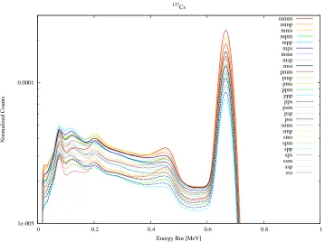
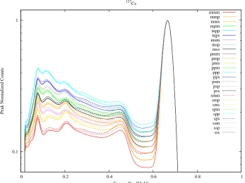
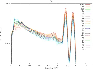
been created along with the post processed detector response parameters, the individ-ual source specifications must be made to simulate the three radioisotopes used in this application. These source specifications included all of the photon emissions from 137_Cs and 60_{Co that were above an intensity of 0.0001. A sample input deck for MCNP of the} sss configuration using137_{Cs as the source can be found in the appendix. All other input} decks will be omitted due to the fact that the variations of the shielding material thick-ness can easily be changed from this base configuration. Upon completing the simulations for all 27 of the variations of thicknesses of the materials for one data set, it was desired to find correlations of the thickness to the changes in the spectra. In order to find these correlations all of the spectra were plotted on one graph. Several trends were appearing but to further exaggerate the connections, each of the spectra were normalized to its own peak value. Figure 3.2 demonstrates the output from MCNP that have been spread using the post processing technique and figure 3.3 shows the peak normalized spectra to the data set using 137_{Cs ranging from the mmm to ppp configurations. Each of the} simulated spectra used 750000000 histories and produced a relative error less than 2% for each energy bin.

(27)

1e-005 0.0001

0 0.2 0.4 0.6 0.8 1

Normalized Counts

Energy Bin [MeV] 137 Cs mmm mmp mms mpm mpp mps msm msp mss pmm pmp pms ppm ppp pps psm psp pss smm smp sms spm spp sps ssm ssp sss

Figure 3.2: Data Set from ’mmm’ to ’ppp’ Configurations using 137_Cs

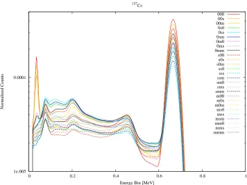
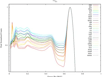
error less than 2% for each energy bin. All subsequent figures depicting various library data sets will maintain the same color schemes and line types in the same order of relative material thickness to the data set as with the previous figures. As with the previous data set, figure 3.4 shows that there are three groupings based off of the thickness of the lead used found along the range from approximately 0.2 to 0.4 MeV. Given the situation that there is no lead shielding present, the low energy photons produced from the source are sufficiently collected but when the higher density shielding materials are added, the collected photons readily decrease. It should also be noted that within these data sets, the unshielded spectrum is included as the 000 case. Figure 3.5 more clearly demonstrates that the lack of shielding material present reduces the individualistic properties of the spectra generated. This has to do with the lack of overall interactions that the photons experience before collection.

(28)

0.1 1

0 0.2 0.4 0.6 0.8 1

Peak Normalized Counts

Energy Bin [MeV] 137 Cs mmm mmp mms mpm mpp mps msm msp mss pmm pmp pms ppm ppp pps psm psp pss smm smp sms spm spp sps ssm ssp sss

Figure 3.3: Peak Normalized Data Set from mmm to ppp Configurations using 137_Cs

Next, the data set using60_{Co ranging from the mmm to ppp configurations are shown.} The source energy intensity and probability distribution were defined within MCNP as follows:

si1 L 1.173237 1.332501

sp1 D 0.999736 0.9998561

Figure 3.7 demonstrates that again there are similarities between the relationships based on the nine different combinations of aluminum and wood and within those groups there are distinctions on the thickness of lead used.

(29)

1e-005 0.0001

0 0.2 0.4 0.6 0.8 1

Normalized Counts

Energy Bin [MeV] 137 Cs 000 00s 00m 0s0 0ss 0sm 0m0 0ms 0mm s00 s0s s0m ss0 sss ssm sm0 sms smm m00 m0s m0m ms0 mss msm mm0 mms mmm

Figure 3.4: Data Set from null to sss Configurations using 137_Cs

5% for each energy bin. Figure 3.8 presents the situation where all of the spectra were tightly grouped together at approximately 0.5 MeV. Below this grouping, similar trends can be seen where the distribution was somewhat based on the thickness of the lead shielding. Compared with the second data set using 137_{Cs, figure 3.9 illustrates that the} null condition to the sss configuration for60_{Co had a much more organized scenario. This} is especially true when considering the spectra below approximately 0.4 MeV.

The spectra generated to create the two data sets using 238_{U as a radioactive source} employed the program GADRAS in generating the distribution of the photon line sources as well as the binned photon groups. GADRAS is a general purpose program used in producing spectra for a wide range of detectors as well as a vast array of source and shielding configurations. It uses a 1D model that combines both ray tracing and SN deterministic transport to rapidly produce a solution a particular problem (Mattingly,

(30)

0.1 1

0 0.2 0.4 0.6 0.8 1

Energy Bin [MeV] 137 Cs 000 00s 00m 0s0 0ss 0sm 0m0 0ms 0mm s00 s0s s0m ss0 sss ssm sm0 sms smm m00 m0s m0m ms0 mss msm mm0 mms mmm

Figure 3.5: Peak Normalized Data Set from null to sss Configurations using 137_Cs

2008). Ray tracing is used to calculate the leakage of the source over a finite energy emitted that are neither scattered nor absorbed. The transport model is used to calculate the individual electron, neutron and photon movements as well as the gamma-day and spontaneous fission gamma photon total final profile (Mitchell, Mattingly). Based on the output from GADRAS, the input source definition used to simulate a 238_{U source in} MCNP can be found in the appendix. Due to the energy range of photons being emitted by the source and the low probability of some of those photons, several of the channels experienced relatively large errors despite 1e9 histories being simulated. When the post processing spreading algorithm was executed, the energy bins that produced relative errors larger than 50% were omitted.

(31)

1e-005 0.0001

0 0.2 0.4 0.6 0.8 1 1.2 1.4 1.6

Normalized Counts

Energy Bin [MeV] 60 Co mmm mmp mms mpm mpp mps msm msp mss pmm pmp pms ppm ppp pps psm psp pss smm smp sms spm spp sps ssm ssp sss

Figure 3.6: Set from mmm to ppp Configurations using60_Co

lead can be made more clearly below approximately 0.3 MeV and became more grouped together above this point. Figure 3.11 was much more difficult to interpret because of the proximity of the entire data set to each other. The same trends were occurring in the order of the aluminum and wood shielding materials but there were few distinctions between each individual spectrum.

The second data set for 238U was created in the exact same manner as the previous data set but with the appropriate shielding thickness. Figure 3.12 clearly shows the most variation between the first data set and the second. This comes from the large distribution of the binned and directly emitted photons from the source as well as the Bremsstrahlung radiation emitted. Figure 3.13 drastically demonstrates the large differences between the two shielding layers of lead and the spectra that have no lead present acting as a shield. This comes from the large intensity of collected photons located at approximately 95 keV

(32)

0.1 1

0 0.2 0.4 0.6 0.8 1 1.2 1.4 1.6

Energy Bin [MeV] 60 Co mmm mmp mms mpm mpp mps msm msp mss pmm pmp pms ppm ppp pps psm psp pss smm smp sms spm spp sps ssm ssp sss

Figure 3.7: Peak Normalized Data Set from mmm to ppp Configurations using60_Co

(33)

1e-005 0.0001

0 0.2 0.4 0.6 0.8 1 1.2 1.4 1.6

Normalized Counts

Energy Bin [MeV]

60_Co 000 00s 00m 0s0 0ss 0sm 0m0 0ms 0mm s00 s0s s0m ss0 sss ssm sm0 sms smm m00 m0s m0m ms0 mss msm mm0 mms mmm

Figure 3.8: Data Set from null to sss Configurations using60_Co

(34)

0.1 1

0 0.2 0.4 0.6 0.8 1 1.2 1.4 1.6

Energy Bin [MeV]

60_Co 000 00s 00m 0s0 0ss 0sm 0m0 0ms 0mm s00 s0s s0m ss0 sss ssm sm0 sms smm m00 m0s m0m ms0 mss msm mm0 mms mmm

(35)

1e-007 1e-006 1e-005 0.0001

0 0.5 1 1.5 2 2.5

Normalized Counts

Energy Bin [MeV]

238_U mmm mmp mms mpm mpp mps msm msp mss pmm pmp pms ppm ppp pps psm psp pss smm smp sms spm spp sps ssm ssp sss

Figure 3.10: Data Set from mmm to ppp Configurations using 238_U

(36)

0.0001 0.001 0.01 0.1 1

0 0.5 1 1.5 2 2.5

Energy Bin [MeV]

238_U mmm mmp mms mpm mpp mps msm msp mss pmm pmp pms ppm ppp pps psm psp pss smm smp sms spm spp sps ssm ssp sss

(37)

1e-007 1e-006 1e-005 0.0001

0 0.5 1 1.5 2 2.5

Normalized Counts

Energy Bin [MeV]

238_U 000 00s 00m 0s0 0ss 0sm 0m0 0ms 0mm s00 s0s s0m ss0 sss ssm sm0 sms smm m00 m0s m0m ms0 mss msm mm0 mms mmm

Figure 3.12: Data Set from null to sss Configurations using 238_U

(38)

0.0001 0.001 0.01 0.1 1

0 0.5 1 1.5 2 2.5

Energy Bin [MeV]

238_U 000 00s 00m 0s0 0ss 0sm 0m0 0ms 0mm s00 s0s s0m ss0 sss ssm sm0 sms smm m00 m0s m0m ms0 mss msm mm0 mms mmm

(39)

Chapter 4 Tri-Linear Interpolation Model

Now that the libraries have been fully constructed, a specialized model must be con-structed for CURMODs use in fitting an input unknown spectrum. Within each data set of libraries, the components that distinguish each spectrum from one another need to be identified. Given that all of the spectra have the same energy bin distribution and bounds, the counts at each channel correspond to the collected photons that have been attenuated or scattered by the specific shielding configurations of lead, aluminum and wood. If the situation where a spectrum was generated with the exact same conditions as one of the libraries, a quick comparison could be made and the shielding material type and thickness could easily be identified. This scenario is very unlikely, so in an attempt to find a solution to the condition where the shielding material thickness within the input spectrum is in-between the thicknesses of the libraries, a model was created that used tri-linear interpolation.

Tri-linear interpolation is an extension of the linear interpolation method but in this instance it extends to three independent variables and approximates the intermediate value within the local axial rectangular prism. In general, consider a unit cube that has

(40)

its origin located at the lower left base corner as shown in figure 4.1 where the values at each vertex is denoted by V000 through V111.

Figure 4.1: Tri-linear Interpolation Method

(41)

Vxyz = V000(1−x)(1−y)(1−z) +

V100x(1−y)(1−z) +

V010(1−x)y(1−z) +

V001(1−x)(1−y)z+

V101x(1−y)z+

V011(1−x)yz+

V110xy(1−z) +

V111xyz (4.1)

The bounding cube will generally not be of unit size nor will it be aligned at the origin but simple translation and scaling of each axis can be used to transform the parameters into and out of the simplified situation.

The tri-linear interpolation used the three independent variables in this problem as the three shielding materials which acted as the direction along which the bounding cube being constructed. The distance along each of the directions corresponded to the thickness of that material. This then dictated that eight of the 27 spectra used in any particular data set were required for this interpolation method to be successful and the location within the defined cube were the thicknesses of the of the input unknown spectrum. The whole data set produces eight separate sectors that were used for material thickness determination. Figure 4.2 shows a physical interpretation of the first data set produced for each radioisotope library where the axes are the materials themselves and the direction along the axes represent the thickness of the corresponding material.

(42)

(43)

Initial guesses are required in CURMOD for the thicknesses of the three materials because these are non-linear parameters and the interpolation was performed at every channel along the spectrum. This scheme also includes a single linear parameter that was used to scale the libraries which can be used to determine the strength of the source.

(44)

Chapter 5 The Test Suite

Ensuring that these methods would work properly and that correct thicknesses of the shielding materials would be calculated, spectra were generated with various thickness of the materials in between the previously generated libraries. It was desired to completely test the tri-linear interpolation scheme, so each of the eight sectors produced by both data sets of 27 libraries received a test input spectrum. Considering that there are six complete data sets where each has eight sectors to be tested, a total of 48 input spectra were produced to be considered as unknown to the solving routine. The thicknesses applied in creating these test unknown spectra can be found in table 5.1 and 5.2 that was used to check the tri-linear method for both of the two data set libraries for each radioisotope. The spectra produced by these different shielding material thicknesses can be found in the following figures.

(45)

Table 5.1: Thicknesses of the Test Spectrum for the First Data Set in Centimeters

Unknown 1 Unknown 5

Pb m-s 0.2 Pb s-p 0.51

Al m-s 1.963 Al m-s 2.1

Wd m-s 5 Wd m-s 6

Unknown 2 Unknown 6

Pb m-s 0.3 Pb s-p 0.5

Al m-s 2 Al m-s 1.463

Wd s-p 8.5 Wd s-p 9.04

Unknown 3 Unknown 7

Pb m-s 0.25 Pb s-p 0.4

Al s-p 3.2 Al s-p 2.6

Wd m-s 4 Wd m-s 4.5

Unknown 4 Unknown 8

Pb m-s 0.19 Pb s-p 0.52

Al s-p 2.8 Al s-p 3.1

Wd s-p 10 Wd s-p 9.4

(46)

0.1 1

0 0.2 0.4 0.6 0.8 1

Energy Bin [MeV] 137 Cs Unknown 1 Unknown 2 Unknown 3 Unknown 4 Unknown 5 Unknown 6 Unknown 7 Unknown 8

Figure 5.1: Peak Normalized Unknown Test Spectra for the First Data Set Using 137_Cs

intensity of the peak produced at approximately 80 keV. Figure 5.2 depicts the same basic trends that occurred in figure 5.1 but in this case the differences were spread out over a larger energy range and there were two primary photo peaks due to 60_{Co being} used.

The spectra produced using238_{U in figure 5.3 demonstrated different trends than} pre-viously generated with the exception being at approximately 100 keV. These differences stem from the distribution of photon line energies emitted as well as the binned distri-bution of grouped photons that correspond to the various mass attenuation coefficients that were adjusted for each of the energies.

The unknown input spectra created to test the second data set that ranged from the null condition to the sss configuration used the following shielding thicknesses.

(47)

Table 5.2: Thicknesses of the Test Spectrum for the Second Data Set in Centimeters

Unknown 1 Unknown 5

Pb 0-m 0.10 Pb m-s 0.20

Al 0-m 1.00 Al 0-m 0.70

Wd 0-m 2.00 Wd 0-m 3.30

Unknown 2 Unknown 6

Pb 0-m 0.05 Pb m-s 0.30

Al 0-m 0.50 Al 0-m 0.30

Wd m-s 6.80 Wd m-s 6.00

Unknown 3 Unknown 7

Pb 0-m 0.15 Pb m-s 0.25

Al m-s 1.50 Al m-s 1.70

Wd 0-m 1.00 Wd 0-m 2.50

Unknown 4 Unknown 8

Pb 0-m 0.08 Pb m-s 0.19

Al m-s 1.80 Al m-s 2.10

Wd m-s 4.80 Wd m-s 7.00

(48)

0.1 1

0 0.2 0.4 0.6 0.8 1 1.2 1.4 1.6

Energy Bin [MeV] 60

Co

Unknown 1 Unknown 2 Unknown 3 Unknown 4 Unknown 5 Unknown 6 Unknown 7 Unknown 8

Figure 5.2: Peak Normalized Unknown Test Spectra for the First Data Set Using 60_Co

same trends in the order of intensity along the Compton continuum but that the overall count differences were much closer in value for all the spectra created.

Again, figure 5.5 demonstrated the similarities in the order of the intensities along the Compton continuum. Also, the backscatter peak in each spectrum at approximately 0.2 MeV had individual shapes that changed depending on the shielding thicknesses.

(49)

0.01 0.1 1

0 0.5 1 1.5 2 2.5

Energy Bin [MeV]

238_U

Figure 5.3: Peak Normalized Unknown Test Spectra for the First Data Set Using238_U

(50)

0.1 1

0 0.2 0.4 0.6 0.8 1

Energy Bin [MeV]

137_Cs

(51)

0.1 1

0 0.2 0.4 0.6 0.8 1 1.2 1.4 1.6

Energy Bin [MeV]

60_Co

Figure 5.5: Peak Normalized Unknown Test Spectra for the Second Data Set Using60_Co

(52)

0.001 0.01 0.1 1

0 0.5 1 1.5 2 2.5

Energy Bin [MeV]

238_U

(53)

Chapter 6 Testing the Tri-Linear Interpolation

Model

Now that two separate complete library data sets have been created for three individual radioisotopes, a model had been generated to make comparisons of an input spectra using tri-linear interpolation and a complete volume of test spectra had been produced to specifically quantify the answers generated, it was only appropriate to perform the tests.

The procedure used to insure the validity of the method was to first choose the input spectrum to test the model. The spectrum produced by MCNP represents a collected yield and as a means to represent a true collected spectrum, all of the counts in each energy bin of the test unknown spectrum were multiplied by 108_{. This scaling factor} represented approximately a 4.5 Ci source collected over a 10 minute period but could be adjusted to either increase or decrease the counts collected to better represent any given situation desired. After the scaling, statistical noise was added to the spectrum to further simulate a true collected spectrum. If the value of the data point was less than 25,

(54)

Table 6.1: Upper Limit Cutoff Values and their Energies for Each Radioisotope

Channel Energy Bin [MeV] 137_Cs ₁₀₃ _0.60819 60_Co ₂₁₄ _1.2573 238_U ₁₅₉ _0.93567

then Poison distributed noise was added which was represented by a whole number. If the data point was larger than the set threshold, Gaussian distributed noise was added which was represented as a continuum of values. At which point the input spectrum was ready to be inspected but before execution, initial guesses for the thicknesses of the materials was required because these are the non-linear parameters within the system. In an ideal condition and as a means to truly test the functionality of the tri-linear interpolation scheme, the initial guesses used were in fact that correct values. This test was designed to ensure the validity of the answers generated rather than the quality of the initial guesses and the adaptability of the method.

The evaluations were limited to only produce a solution from the first channel to a location that was used to help disassociate the high degree of correlation at the full energy photo peaks. This location first considered the highest energy identifying photo peak for the particular radioisotope, its FWHM was then calculated and the upper limit of evaluation was placed twice the FWHM below its corresponding peak. These cutoff points were predetermined and their values can be found in the following table.

(55)

Figure 6.1: Interpretation of the Sector for Unknown 1 in the First Data Set

(56)

The example used was located in the lower most shielded condition sector for the first data set library which ranged from the mmm configuration to the sss configuration. The ranges of configurations act as the bounds used in the tri-linear interpolation and the initial guesses act as the location within the cube where the value was desired to be found.

(57)

Table 6.2: Thicknesses of the Test Spectrum for the First Data Set in Centimeters

Trial ChiSqur Material Thickness %Sigma Material Thickness %Sigma Material Thickness %Sigma Parameter Value %Sigma

1 0.8119 Pb= 2.36E-01 1.70E-02 Al= 1.82E+00 4.68E-02 Wood= 5.75E+00 6.82E-02 Linear= 1.03E+08 1.82E-03

AVERAGE= 1.07E+00 2.00E-01 1.74E-02 1.99E+00 3.87E-02 4.76E+00 7.68E-02 1.00E+08 1.82E-03

(58)

Table 6.2 demonstrates 30 individual solutions that were produced. Each of the an-swers produced a χ2 that represents a valid solution to the input unknown problem and based on the averages generated, the found thicknesses for lead and aluminum were very close to the exact answer of 0.2 and 1.963 cm respectively. The value found for wood was within one standard deviation to the true solution of 5 cm. Also, the linear fitting parameter was very close to the true value with very good statistical confidence. Figure 6.2 illustrates the found solution for the 30th _{trial in the previous table.}

-500 0 500 1000 1500 2000 2500 3000 3500 4000 4500

0 20 40 60 80 100 120

Counts

Channel Number

Input ’Unknown’ Spectrum Output ’Found’ Spectrum Residuals

Figure 6.2: Tri-Linear Fit for the 30th _{Trial in Table 6.2}

(59)

of libraries.

(60)

Table 6.3: Averages of 30 Trials with the First Data Set Using137_Cs

Pb Al Wood Amount

χ2 TRUE Meas. σ(%) TRUE Meas. σ(%) TRUE Meas. σ(%) Meas. σ(%)

unk1 1.071 0.20 0.20 1.74 1.96 1.99 3.87 5.00 4.76 7.68 1.00E+08 0.18

unk2 1.024 0.30 0.29 1.37 2.00 2.14 4.60 8.50 7.92 4.82 9.99E+07 0.19

unk3 1.038 0.25 0.25 1.39 3.20 3.19 2.26 4.00 4.06 9.15 9.99E+07 0.19

unk4 1.031 0.19 0.19 3.53 2.80 2.85 4.07 10.00 9.89 4.69 1.00E+08 0.18

unk5 1.072 0.51 0.51 0.87 2.10 2.00 5.29 6.00 6.29 7.68 9.98E+07 0.21

unk6 1.093 0.50 0.49 1.52 1.46 1.48 11.42 9.04 8.92 6.91 9.94E+07 0.21

unk7 1.020 0.40 0.40 1.27 2.60 2.60 3.72 4.50 4.44 10.33 1.00E+08 0.20

unk8 1.079 0.52 0.52 1.15 3.10 3.05 4.27 9.40 9.77 5.50 9.93E+07 0.22

Averagesσ(%) 1.60 4.94 7.10 0.20

(61)

Table 6.4: Averages of 30 Trials with the First Data Set Using60_Co

Pb Al Wood Amount

unk1 1.023 0.20 0.21 3.70 1.96 1.85 6.04 5.00 5.58 9.20 1.00E+08 0.15

unk2 1.021 0.30 0.29 2.67 2.00 2.13 5.09 8.50 7.98 5.99 1.00E+08 0.15

unk3 1.016 0.25 0.25 2.39 3.20 3.19 2.64 4.00 4.13 10.32 1.00E+08 0.15

unk4 1.016 0.19 0.19 5.61 2.80 2.77 4.69 10.00 10.20 5.27 1.00E+08 0.15

unk5 1.043 0.51 0.51 1.31 2.10 2.08 5.12 6.00 6.05 8.10 1.00E+08 0.16

unk6 1.058 0.50 0.50 2.19 1.46 1.53 10.74 9.04 8.79 7.31 1.00E+08 0.15

unk7 1.017 0.40 0.41 1.68 2.60 2.54 3.55 4.50 4.79 8.53 1.00E+08 0.15

unk8 1.066 0.52 0.52 1.74 3.10 3.15 4.09 9.40 9.22 6.17 1.00E+08 0.16

Averagesσ(%) 2.66 5.24 7.61 0.15

Absolute Average Error 4.73E-03 5.95E-02 2.75E-01 1.53E+05

(62)

Table 6.5: Averages of 30 Trials with the First Data Set Using238_U

Pb Al Wood Amount

unk1 1.042 0.20 0.20 2.06 1.96 2.00 5.79 5.00 4.64 12.61 9.99E+07 0.18

unk2 1.023 0.30 0.31 1.36 2.00 1.90 6.32 8.50 8.71 6.33 9.91E+07 0.20

unk3 1.015 0.25 0.26 1.54 3.20 3.17 3.29 4.00 3.87 14.28 9.92E+07 0.20

unk4 1.080 0.19 0.19 3.56 2.80 2.82 4.99 10.00 9.99 6.04 9.97E+07 0.19

unk5 1.075 0.51 0.51 1.02 2.10 2.06 7.08 6.00 6.10 11.58 9.96E+07 0.22

unk6 1.043 0.50 0.50 1.35 1.46 1.44 12.04 9.04 9.03 7.76 9.93E+07 0.22

unk7 1.032 0.40 0.40 1.44 2.60 2.57 5.02 4.50 4.56 12.95 9.96E+07 0.21

unk8 1.012 0.52 0.51 1.05 3.10 3.25 3.90 9.40 8.79 6.93 9.98E+07 0.23

Averagesσ(%) 1.67 6.05 9.81 0.21

(63)

The solutions for the first data set proved as an overall success. The measured thick-nesses for lead were extremely close with the largest discrepancy between the true and calculated value as 0.01 cm. Aluminum was also relatively close in value with the largest difference being 0.15 cm and wood with the largest inexact value off by 0.61 cm. These differences were experienced using 238_{U and the spectrum Unknown 8 which can be} at-tributed to the shielding material thicknesses of this test being close to the bounding edges of the tri-linear interpolation. Also, the variations in the shielding present have significantly distorted the spectra for 238_{U from the large distribution and probabilities} of the emitted radiation. With all of these distortions being present, the linear fitting amount is again close to the true value of 1E8 and a good representation of the activity for the found source used could be made. Its associated error is also small which denotes the overall confidence in the found solution for this linear parameter.

As before, 30 trials of the same test unknown spectra were performed and then aver-aged but in the following tables, the second data set of libraries was used and therefore generated another set of 24 averages with statistical values. These configurations ranged from the null condition to the sss configuration.

(64)

Table 6.6: Averages of 30 Trials with the Second Data Set Using137_Cs

Pb Al Wood Amount

unk1 1.505 0.10 0.00 224.34 1.00 0.48 8.61 2.00 0.08 251.98 1.06E+08 0.18

unk2 2.878 0.05 0.09 1.10 0.50 0.00 NaN 6.80 3.67 2.30 1.03E+08 0.17

unk3 17.552 0.15 0.10 10.35 1.50 1.18 0.50 1.00 0.91 17.51 9.03E+07 0.18

unk4 1.409 0.08 0.04 5.03 1.80 1.74 2.36 4.80 1.58 7.73 1.05E+08 0.17

unk5 1.278 0.20 0.25 1.26 0.70 0.55 8.59 3.30 0.10 13.64 1.04E+08 0.18

unk6 1.134 0.30 0.29 1.11 0.30 0.59 10.71 6.00 4.86 4.56 1.00E+08 0.19

unk7 1.056 0.25 0.27 1.06 1.70 1.60 2.68 2.50 0.87 27.14 1.02E+08 0.19

unk8 1.081 0.19 0.19 2.02 2.10 2.09 3.85 7.00 6.81 5.52 1.00E+08 0.18

Averagesσ(%) 30.78 5.33 41.30 0.18

(65)

Table 6.6 demonstrates very poor solutions for all of the spectra except for Unknown 8. The primary reason for these drastic discrepancies between the first and second data set arrangement solutions stem from the lack of shielding experienced. Given the low energy photons were not attenuated as much, the collected spectra differ quite largely and these differences cause the tri-linear interpolation model to achieve a less than desirable solution and these differences can be seen in the library used in figures 3.4 and 3.5. The poor results for each of the shielding material thicknesses are shown in the averages for the percent of standard deviations having large values from the inability to resolve the parameters. One answer to help resolve this issue was to ignore the low energy portion of the libraries and collected spectra and in this case that threshold was placed at the 13th _{channel which was at approximately 80keV.}

(66)

Table 6.7: Averages of 30 Trials with the Second Data Set Using137_{Cs Over a Reduced Range}

Pb Al Wood Amount

unk1 1.281 0.10 0.01 62.00 1.00 0.47 10.37 2.00 0.41 90.02 1.06E+08 0.19

unk2 1.290 0.05 0.09 3.18 0.50 0.47 13.77 6.80 5.90 5.52 1.05E+08 0.18

unk3 1.353 0.15 0.00 62.46 1.50 0.00 NaN 1.00 1.71 8.24 1.02E+08 0.19

unk4 1.084 0.08 0.04 15.66 1.80 1.56 8.41 4.80 4.95 32.08 1.04E+08 0.20

unk5 1.151 0.20 0.24 1.67 0.70 0.48 10.50 3.30 0.41 61.19 1.04E+08 0.20

unk6 1.002 0.30 0.29 1.20 0.30 0.59 11.90 6.00 4.82 4.63 9.99E+07 0.20

unk7 0.957 0.25 0.27 1.28 1.70 1.59 2.80 2.50 0.91 28.92 1.02E+08 0.20

unk8 0.879 0.19 0.19 2.09 2.10 2.13 4.14 7.00 6.66 6.0 3 1.00E+08 0.19

Averagesσ(%) 18.69 8.84 29.58 0.19

(67)

Reducing the range over which the tri-linear interpolation does assist in choosing the correct values in most cases. The channels over which the evaluation occurs could be adjusted depending on the radioisotope and the total amount of collected photons. In general, the tri-linear approach does not produce reputable solutions when there is little shielding material present in the spectrum. However, the solutions generated that produce aχ2 _{close to 1 place the thicknesses of the material within the appropriate bounds of the} library which still holds useful information with the only exception of Unknown 3 in the previous table.

(68)

Table 6.8: Averages of 30 Trials with the Second Data Set Using60_{Co Over the Full Range}

Pb Al Wood Amount

unk1 1.076 0.10 0.02 19.21 1.00 0.43 14.75 2.00 0.37 101.26 1.02E+08 0.14

unk2 1.128 0.05 0.10 3.56 0.50 0.21 49.42 6.80 4.43 11.23 1.02E+08 0.14

unk3 1.033 0.15 0.01 127.76 1.50 1.36 2.94 1.00 1.90 11.11 1.01E+08 0.14

unk4 1.041 0.08 0.04 9.49 1.80 1.45 5.51 4.80 6.11 6.77 1.01E+08 0.14

unk5 1.095 0.20 0.22 2.36 0.70 0.50 11.90 3.30 0.16 603.07 1.01E+08 0.14

unk6 1.063 0.30 0.32 2.50 0.30 0.72 14.15 6.00 5.42 6.81 1.01E+08 0.15

unk7 1.052 0.25 0.27 1.57 1.70 1.58 2.79 2.50 0.51 49.90 1.01E+08 0.15

unk8 1.007 0.19 0.19 2.74 2.10 2.11 2.98 7.00 7.00 4.35 1.00E+08 0.15

Averagesσ(%) 21.15 13.06 99.31 0.14

(69)

The results for the second data set for 60_{Co were better in general than the results} found for137_{Cs. This was because with this new source, there were no lower energies being} emitted and therefore the differences between each of the libraries diminished. Since the highest energy was being used to locate the upper limit of the evaluations, the second full energy peak was used in the fitting routine which gives a higher degree of correlation than if just the portion of the spectrum that had the Compton continuum was considered. Also, the total number of channels considered was larger than previously used.

(70)

Table 6.9: Averages of 30 Trials with the Second Data Set Using238_{U Over a Limited Range}

Pb Al Wood Amount

unk1 1.327 0.10 0.10 0.86 1.00 0.78 3.36 2.00 3.48 4.40 8.80E+07 0.18

unk2 1.069 0.05 0.10 1.43 0.50 0.09 738.51 6.80 6.32 41.08 1.04E+08 0.18

unk3 1.140 0.15 0.00 38.82 1.50 1.06 11.35 1.00 7.15 9.04 1.06E+08 0.19

unk4 1.186 0.08 0.07 8.39 1.80 1.56 20.84 4.80 6.83 27.35 1.02E+08 0.19

unk5 0.833 0.20 0.31 1.20 0.70 0.00 81726.35 3.30 1.40 39.00 1.05E+08 0.20

unk6 0.830 0.30 0.25 1.07 0.30 1.07 8.98 6.00 5.14 7.90 9.48E+07 0.21

unk7 0.807 0.25 0.28 2.69 1.70 1.38 13.61 2.50 2.33 41.97 1.02E+08 0.21

unk8 0.813 0.19 0.19 3.28 2.10 2.09 7.18 7.00 6.96 10.40 9.96E+07 0.21

Averagesσ(%) 7.22 10316.27 22.64 0.20

(71)

As with using 137_{Cs as a source,} 238_{U also required a lower level discriminator be} applied before analyzing the input unknown spectra. This cut off level was placed at the 32nd _{channel at approximately 195 keV and chosen because of its ability to remove the}

largest low energy feature. It should be noted that in some of the 30 trial runs of the initial input spectra, the tri-linear model did not always generate answers that could be resolved. This aspect of the solution was attributed to the noise produced by the testing algorithm to simulate a realistic spectrum and thusly if the spectra had larger counts collected the signal to noise ratio would be reduced and solutions could be found. An interesting feature of the tri-linear interpolation was that the solution to the problem was not always correct in its evaluations. The thicknesses of the materials might have been incorrect but the overall fit was successful and could easily be seen in the reduced χ2

to the input spectrum. Also, despite the correctness of the thicknesses of the materials, the linear fitting parameter was proven to be accurate and therefore the source strength could be properly accessed. Given no initial information about the input spectrum, these fits to the problem then become a viable solution to the shielding thickness despite their incorrectness.

(72)

Chapter 7 Fully Automated Shielding

Thickness Determination

The tri-linear model used in the MCLLS method demonstrated that it could generate reasonable solutions for determining the thicknesses of lead, aluminum and wood given the correct initial guesses. This ability is the foundation of the work proposed here but in order for this to be put to practical use, initial guesses for the non-linear parameters must be automatically made. The automated aspect of the initial guess making process is essential because it allows a wider variety of end users to operate a final product that could use this technique.

(73)

technique. It began by finding the peak locations of spectra used when calibrating the detector to convert from channel number to energy bin. These calibration spectra were created using the same source location that the previous libraries used but in this case all of the shielding material was removed. The sources used in this development were 22_Na, 60_Co, 137_Cs, 133_{Ba and} 238_{U but in reality, any combination of sources and their} associated peaks could be used.

Finding each of the peaks within each individual spectrum made use of the second derivatives based on the Gaussian distribution. The 1D second derivatives of a Gaussian were determined over a range of ±five channels from the point in consideration and the standard deviation of the fit had been chosen as 1E8 which was regarded as significantly large. The basic equations used were as follows:

g(x) = e−x2

2σ2 (7.1)

g0₍_x_{) =} ₋ 1

2σ22xe

−x2

2σ2 =−

x σ2e

−x2

2σ2 (7.2)

g00₍_x_{) = (}x

2

σ4 − 1 2σ2)e

−x2

σ2 (7.3)

This type of differentiation was chosen because if the standard deviation was reduced and the range of channels about the center point was altered, then the differentiation acts similar to a smoothing algorithm. Both of these parameters could be adjusted as needed to either increase or decrease the amount of smoothing used before further calculations were performed.

After the derivatives have been calculated along the entire spectrum, the peaks were then searched for. This was done by using the locations where these derivatives experience a local minimum. The location was found by locating a single channel where the average

(74)

of the five derivatives to the left of the point in question was negative and the average of the five derivatives to the right of the point in question was positive. This gives several possibilities of peak locations that can be attributed to the statistical noise within the spectra and the averaging of the derivatives. As a means to pick the most appropriate location, the derivative with the lowest value was chosen as a rough estimate of the peak location over a similarly grouped local minimum location.

(75)

error. As before, the value of the cutoff could be adjusted to fit any given situation. All of the processes were repeated for every unshielded calibration file and for every found peak within each spectrum but this did not guarantee finding all of the peaks. This was because the end goal was to produce a table of centroid peaks and their associated FWHM with a high degree of confidence in their values to make comparisons with when the input unknown spectrum is treated. These judgments were made by creating a second order power series fit of the centroid to their associated FWHM.

y(x) = eCxAln(x)+B (7.4) Where A, B, and C were the found empirical constants as 0.8951, -2.053 and -0.0417 respectively. This type of equation was chosen to better fit the known non-linearity that NaI(Tl) detectors experience between the deposited energy of the incident particle and the response recorded. Figure 7.1 demonstrates the relationship that was automatically generated between the found peaks and their associated FWHM though using the second order power series fit.

Now that an equation had been created, the input unknown spectrum peak values were searched for and their corresponding FWHM were found in the same fashion as the calibration spectra. Again, as with the calibration spectra, the cutoff could be adjusted to find the most accurate locations but for this application, it had been determined as 1000.0. In this instance, when the peaks for the input spectrum were found and characterized, they were compared to the centroid values and the FWHM of the unshielded calibration spectra. After identifying the peak, if the difference in the FWHM of the found centroid to the fitted second order power series equation was greater than 0.05, then the peak was

(76)

0 1 2 3 4 5 6 7

0 100 200 300 400 500

FWHM

Channel Number

2nd Order Power Series Fit Calibration Spectra Peaks and their FWHM

Figure 7.1: Peaks VS FWHM and the 2n_d _{Order Power Series Fit}

considered convolved and is then skipped. This was done to choose the correct library to later decide the shielding material thicknesses and to determine if there was a shielded library for the peaks found within the spectrum. Next, this portion of the program then strips out the un-attenuated library from the input spectrum from using a ratio of the heights of the centroid values in both spectrums. It then returns the value that the library was multiplied by along with an updated spectrum where zeros have been entered above the highest channel in the library to reduce later confusion with finding a solution.

(77)

situation that the residuals were statistically defined as noise, the program stops but if the program finds that the residuals have a distinctive shape and the linearly stripped radioisotope had a corresponding shielded library, the program moves onto a non-linear search of the shielding materials.

The search for the shielding materials began by attempting to choose estimates for each of the eight sectors created by the 27 libraries. These sectors formed from the three thicknesses of the three shielding materials. Determinations of the initial estimates for the thicknesses began by fitting the peak heights of all 27 spectra within the library to the found peak centroid within the unknown spectrum. The scaling multipliers for each spec-trum were recorded. Then, analysis of an upper limit to the channels was automatically calculated. As with the testing phase of the previous chapter, this calculation began by determining what the FWHM of the identifying centroid value was by using the second order power series fit that was previously created. The limit was then set as twice the distance of the calculated FWHM below the corresponding centroid value. This location was selected as a means to help disassociate the high degree of correlation that all 27 spectra have about the peak and to focus more on the interactions of the gamma parti-cles which were more indicative of the shielding materials. The residuals of the peak fit solution from channel 0 to the upper limit were then averaged for each of the 27 libraries and the results were recorded. Also, as a means to help predetermine the appropriate thicknesses, the program CEARLLS (another CURMOD application) was automatically executed for an input of the unknown spectrum and each of the 27 libraries peak fits from channel 0 to the upper limit. CEARLLS performs a full spectrum linear fit for each of the libraries about the entire range permitted to the input unknown spectrum and produced results for: the scaling factor, the percent of the standard deviation, R, the percent of the area that was covered, the χ2 of the fit and the average of the residuals.

(78)

These partial solutions were able to produce an initial rough estimate of the sector that the input spectrum resides in which helps to define the range of each of the materials thickness.

Now that each of the spectra within the library had an associated value of how well it fits the input spectrum, an interpolation was made within each of the eight sectors. This was done by using tri-linear interpolation where the limits of the bounds were determined by the thicknesses of the materials that define each sector. The point of interpolation was determined by producing a fraction in each direction that corresponds to the material based off of the absolute value of the average of the residuals from the peak fit. This fraction was the sum of the four lower defining bound averages over the sum of all eight edges of the sector. Each material fraction in each sector was comprised of the same eight values but the arrangement of the lower bounds for each material was different. Once the fractions have been determined, the tri-linear interpolation occurs at each channel and a new spectrum was produced. This entire process was repeated for each of the eight sectors. As with the 27 library spectra, results were produced when each of the eight sectorss interpolated spectra were fit at the peak centroid and also through application of CEARLLS from channel 0 to the channel defined by the upper limit.

(79)

answer.

The first test case chooses the sector that had the lowest average residual value from the peak fitting process and its sister test chose the sector that has the lowest average residual value from the CEARLLS program. These two tests were weighted equally. The next test series that was weighted slightly less than the previous tests used the statistical outputs generated from CEARLLS. These tests chose the sector that had the smallest value for the percent of standard deviation and the χ2 that was closest to a value of one. Also, these tests chose the sector with the highest value for R and the percent of the area under the curve that was successfully fit.

After making these initial choices, the next step was to consider the residuals created when the eight sectors interpolated spectra were subtracted from the input unknown spectrum when the interpolated spectra were fit to the defining peak. A linear fit was then created upon each of the residuals and the statistical values of the total sum of squares and the residual sum of squares are determined. The idea was that the sector that had the best fit will have the lowest slope, y-intercept and both statistical values. Each sector that had the lowest of each of these parameters receives a winning choice value where the slope and y-intercept are weighted slightly less than the statistical successes. If the sector receives a value for the absolute value of the y-intercept of the linear fit to the residuals that was larger than is the identifying peak centroid height raised to the 2/3, the sector was then rejected for later analysis. This was done as a means to help remove sectors that had no relevance to solving the problem of the unknown thicknesses of shielding materials.

The last analysis performed before determination of the most correct sector and sub-sequent thickness, involved the tri-linear interpolation model of the MCLLS technique where three materials act as the three coordinates and each direction was the