Construction of a Genetic Linkage Map in Tetraploid Species Using Molecular Markers

Copyright2001 by the Genetics Society of America

Construction of a Genetic Linkage Map in Tetraploid Species Using

Molecular Markers

Z. W. Luo,*

_{C. A. Hackett,}

_{J. E. Bradshaw,}

_{J. W. McNicol}

_{and D. Milbourne}

*School of Biosciences, The University of Birmingham, Birmingham B15 2TT, England,†_{Laboratory of Population and Quantitative Genetics,}

Institute of Genetics, Fudan University, Shanghai 200433, China and‡_{Biomathematics and Statistics Scotland,} §_{Scottish Crop Research Institute, Invergowrie, Dundee, DD2 5DA, Scotland}

Manuscript received May 1, 2000 Accepted for publication November 30, 2000

ABSTRACT

This article presents methodology for the construction of a linkage map in an autotetraploid species, using either codominant or dominant molecular markers scored on two parents and their full-sib progeny. The steps of the analysis are as follows: identification of parental genotypes from the parental and offspring phenotypes; testing for independent segregation of markers; partition of markers into linkage groups using cluster analysis; maximum-likelihood estimation of the phase, recombination frequency, and LOD score for all pairs of markers in the same linkage group using the EM algorithm; ordering the markers and estimating distances between them; and reconstructing their linkage phases. The information from different marker configurations about the recombination frequency is examined and found to vary consider-ably, depending on the number of different alleles, the number of alleles shared by the parents, and the phase of the markers. The methods are applied to a simulated data set and to a small set of SSR and AFLP markers scored in a full-sib population of tetraploid potato.

G

involved in modeling polysomic inheritance can be and for a large number of diploid plant and

ani-mal species. In contrast, mapping studies in polyploid avoided. These involve either the use of single-dose

(sim-plex) dominant markers (e.g., AFLPs and RAPDs) that

species are much less advanced, partly due to the

com-plexities in analysis of polysomic inheritance as demon- segregate in a simple 1:1 ratio in segregating

popula-tions or use of the corresponding diploid relative as an

strated in, for example,Mather (1936), De Winton

and Haldane (1931), Fisher (1947), and Bailey approximation to the polyploid case (Bonierbaleet al.

1988;Gebhardtet al.1989). More recently,Hackett

(1961). The development of DNA molecular markers

[restriction fragment length polymorphisms (RFLPs), et al. (1998) presented a theoretical and simulation

study on linkage analysis of dominant markers of differ-amplified fragment length polymorphisms (AFLPs),

randomly amplified polymorphic DNAs (RAPDs), sim- ent dosages in a full-sib population of an autotetraploid

species, and this approach was used by Meyer et al.

ple sequence repeats (SSRs), and single nucleotide

poly-(1998) to develop a linkage map in tetraploid potato. morphisms (SNPs), etc.] and advances in computer

The use of codominant markers, particularly those technology have made both theoretical and

experimen-with a high degree of polymorphism such as SSRs, is tal studies of polysomic inheritance much more feasible

known to improve the efficiency and accuracy of linkage than ever before. Some of these markers have recently

analysis in diploid species (Terwilliger et al. 1992;

been used as a fundamental tool to construct genetic

JiangandZeng 1997). In polyploid species, the rela-linkage maps in polyploid species that display polysomic

tionship between the parental genotype and the

pheno-inheritance (Al-Janabiet al.1993;Da Silvaet al.1993;

type as shown by the gel band pattern is less clear-cut,

Yu and Pauls 1993; Hackett et al. 1998; Brouwer

due to the possibilities of different dosages of alleles, andOsborn1999), to search for quantitative trait loci

and this provides extra complexity as explained inLuo

(QTL) affecting disease resistance in tetraploid potato

et al.(2000). The aim of the present study is to develop (Bradshawet al.1998;Meyeret al.1998), and to

investi-methodology for constructing linkage maps of codomi-gate population structure in autotetraploid species

nant or dominant genetic markers in autotetraploid (Ronfortet al.1998).

species under chromosomal segregation, i.e., the

ran-Due to a lack of well-established theory for mapping

dom pairing of four homologous chromosomes to give genetic markers in polyploid species, much research

two bivalents. The complications arising from quadriva-lent or trivaquadriva-lent plus univaquadriva-lent formation are not consid-ered in this article. A series of problems involved in

Corresponding author:Z. W. Luo, School of Biosciences, The

Univer-tetrasomic linkage analysis are addressed. Statistical

sity of Birmingham, Edgbaston, Birmingham B15 2TT, United

King-dom. E-mail: zwluo@bham.ac.uk properties of the methods are investigated by theoretical

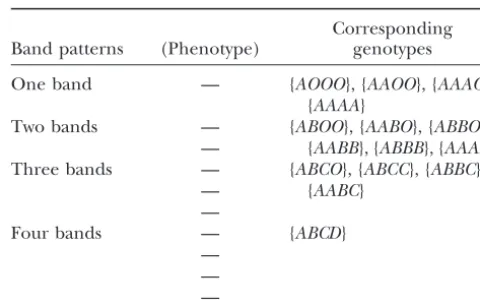
TABLE 1

analysis or simulation study, and some experimental

data from a tetraploid potato study are used to illustrate _{The relationship between marker phenotypes and genotypes}

the use of the theory and methods in analyzing breeding _{at a single locus for an individual}

experiments.

Corresponding Band patterns (Phenotype) genotypes THEORY OF LINKAGE MAP CONSTRUCTION

One band — {AOOO}, {AAOO}, {AAAO},

Model and notation:The theoretical analysis consid- _{AAAA}

ers a full-sib family derived from crossing two autotetra- Two bands — {ABOO}, {AABO}, {ABBO},

— {AABB}, {ABBB}, {AAAB}

ploid parental lines. LetMi(i⫽1 . . .m) bemmarker

Three bands — {ABCO}, {ABCC}, {ABBC},

loci (with dominant or codominant inheritance). Let

— {AABC}

G1 andG2be the genotypes at the marker loci for two

—

parental individuals, respectively.Gi (i ⫽ 1, 2) can be

Four bands — {ABCD}

expressed as a m ⫻ 4 matrix. Because two tetraploid _—

individuals have at most eight distinct alleles, we repre- _—

sent each element of Gias a letterA–HorO, where O —

represents the null allele due to mutation within primer

Different letters represent different alleles andOdenotes

sequences (see, for example,Callenet al. 1993). It is _{the null allele.}

important to note that allele A at marker locus 1 is

different from alleleAat marker locus 2.

When we are considering linked loci, it is often neces- distinguished from a single dosage on the basis of the

sary to specify how the alleles at different loci are gel band pattern. Second, some alleles may not be

re-grouped into homologous chromosomes,i.e., the link- vealed as the presence of a corresponding gel band,i.e.,

age phases of the alleles. Alleles linked on the same the null alleles. Table 1 summarizes the relationship

homologous chromosome will appear in the same col- between genotype and phenotype at a marker locus

umn of the matrixGi.For a two-locus genotype with four in which all possible cases of null alleles and multiple

different alleles at each locus, one possible genotype is dosages of identical alleles are taken into account. It

can be seen from Table 1 that there may be four, six,

冢

ABCD

冣

individual genotype can be uniquely inferred from its

This indicates that allele Aof locus 1 is on the same

phenotype if and only if the individual carries four

dif-chromosome as allele Aof locus 2, allele Bof locus 1

ferent alleles and these alleles are also observed as four

is on the same chromosome as alleleBof locus 2, etc.

distinct bands. Alternatively we could have a genotype matrix, for

ex-Luo et al. (2000) recently developed a method for ample,

predicting the probability distribution of genotypes of a pair of parents at a codominant (for example, RFLPs,

冢

BACD

冣

RAPDs) marker locus on the basis of their and their

In this case alleleAof locus 1 is on the same

chromo-progeny’s phenotypes scored at that locus. This

ap-some as alleleBof locus 2, etc. If the phase is uncertain,

proach infers the number of possible configurations of alleles will be enclosed in parentheses. For brevity in

the parental genotypes with the corresponding proba-the text of this article, two-locus genotypes of known

bilities, conditional on the parental and offspring phe-phase are also written using a slash to separate the

chro-notypes. For each of the predicted parental genotypic mosomes, so that the above genotypes would be written

configurations, the expected number of offspring

phe-asAA/BB/CC/DDandAB/BA/CC/DD, respectively.

notypes and their frequencies can be calculated and

We defineP1andP2to be the phenotypes of the two

compared to the observed frequencies. Results from

parents,i.e., their gel band patterns at the marker loci.

a simulation study and analysis of experimental data

Pi (i⫽ 1, 2) can be denoted by a m⫻ 8 matrix, each

showed that in many circumstances both the parental of whose elements may take a value of 1 indicating

genotypes can be correctly identified with a probability presence of a band at the corresponding gel position

of nearly 1. A tetrasomic linkage analysis can then be or 0 indicating absence of a band. These matrices carry

carried out using the most probable parental genotype,

no information about phase. Thejth rows of GiandPi

or using each of a set of possible parental genotypes in

correspond to locusMj.LetOMibe then⫻8 matrix of

turn if more than one genotype is consistent with all

phenotypes of thenoffspring at the marker locus Mi.

the phenotypic data. This is illustrated in the following In general, there is no simple one-to-one relationship

analyses of data from simulation and experimental between the phenotype and the genotype of markers

studies. scored in tetraploid individuals. There are two reasons

of the parental genotype(s) that is consistent with the of configurations, linkage phases, and true

recombina-tion frequencies. For true recombinarecombina-tion frequenciesrⱕ

parental and offspring phenotype data using the

method described inLuoet al.(2000); (ii) the detection 0.2, the power was generally 100% (i.e., the

hy-pothesis of independent segregation was always re-of linkage between pairs re-of marker loci and their

parti-tion into linkage groups; (iii) the estimaparti-tion of linkage jected) for a significance level␣ ⫽0.01 and⬎90% for

rⱕ0.3. The exceptions to this were configurations with

phase, recombination frequency, and LOD score for

pairs of markers within each linkage group; and (iv) alleles restricted to simplex repulsion or duplex mixed

configurations;e.g., for crossAB/AA/BA/BB⫻CC/CD/

the ordering of markers within each linkage group. The

power to detect linkage and the variance of the estimates DD/DC, with all alleles in duplex mixed configurations,

and a true recombination frequency of 0.2, indepen-of the recombination frequency are shown to vary

con-siderably with parental configuration and phase, and dent segregation was rejected for 3/100 simulations.

When the markers were genuinely unlinked, the rejec-this will be examined.

Test for independent segregation of loci: The first tion rate for a significance level␣ ⫽0.05 was found to be close to 5% for all configurations examined. step of the linkage analysis is to test whether pairs of

loci are segregating independently. We propose that Partition of loci into linkage groups:Cluster analysis

is a suitable technique to partition the marker loci into this may be investigated for each pair of markers by

representing their joint segregation in a two-way contin- linkage groups, so that a marker segregates

indepen-dently of markers in different linkage groups and shows gency table and testing for independent segregation, as

discussed by various authors (e.g., Maliepaard et al. a significant association with at least some of the other

markers within its linkage group. The above test statistics

1997) for diploid crosses. Letnijbe the observed number

of progeny with the ith (i ⫽ 1, 2, . . . , I) marker depend on the number of marker phenotypes at each

locus, but the significance level of the test for

indepen-phenotype at the first locus and thejth(j⫽1, 2, . . . ,

J) marker phenotype at the second locus. The expected dent segregation is comparable for all pairs and could

be regarded as a distance between loci. Although it

number under independent segregation iseij⫽ni·n·j/n,

where ni· ⫽RJj⫽1nijandn·j⫽ RIi⫽1nij. The observed and ranges from 0 for the most tightly linked loci to 1, the

range (0, 0.05) is of most interest for indicating pairs expected numbers may be compared by Pearson’s

chi-square statistic, of loci that are likely to be linked. We therefore prefer

to transform the significance level, says, to a measure

of distance that gives more discrimination between the ␹2⫽

兺

I

i⫽1

兺

J

j⫽1

(nij⫺eij)2

eij

. (1)

distances of most interest. The transformationd⫽1⫺

10⫺2s_{, which maps the range of the significance level (0,}

Other possible test statistics are the likelihood-ratio test

0.05) to the range of the distance measure (0, 0.21), was used here, although many alternative

transforma-G2⫽₂

兺

I

i⫽1

兺

J

j⫽1

nijlog

nij

eij

(2)

tions are possible. Different clustering methods will give slightly different dendrograms: the nearest-neighbor

or the Cressie-Read family of power divergence statistics _{cluster analysis adds a marker to a cluster according to}

its distance to the closest marker in the cluster, but can

C(␭)⫽ 2 ␭(␭ ⫹1)

兺

I

i⫽1

兺

J

j⫽1

nij

冤冢

nij

eij

冣

␭

⫺1

冥

from each subgroup. We prefer to compare the dendro-gram from nearest-neighbor cluster analysis with that These statistics have an asymptotic chi-square

distribu-tion with d.f.⫽(I⫺1)(J⫺1). However, in this applica- from average linkage cluster analysis to avoid such

“chaining.” Inspection of the clustering at distances cor-tion the contingency tables may be sparse, as the

num-ber of cells can be as large as 362 _{⫽ 1296, and so the responding to different levels of significance will}

indi-cate how the marker loci should be partitioned into asymptotic distribution cannot be assumed without

in-vestigation. Table 2 compares the percentage points for

the distribution of ␹2_{, G}2_{, and C(}␭_{) with} ␭ ⫽ 2_⁄

3 [as

TABLE 2

recommended byCressieandRead(1984) for sparse

Percentage points for the distribution of 500 replicates of

tables] for 500 simulations of the configurationAA/BB/

test statistics for independent segregation of two loci with

CC/DD⫻EE/FF/GG/HH, with the two loci segregating

parental genotypesAA/BB/CC/DD⫻EE/FF/GG/HH

independently and 200 offspring. The percentage points for Pearson’s chi-square statistic are closest to

Percentage point True ␹2 _G2 _{C(␭ ⫽}2_⁄ 3)

the true values, but the other two have lower percentage

points. The three distributions were compared for sev- 0.25 1191 1177 703 892

0.50 1225 1213 715 915

eral other configurations, but Pearson’s chi-square

sta-0.75 1257 1249 726 934

tistic always had percentage points closest to the true

0.95 1304 1295 740 959

distribution.

The power of Pearson’s chi-square test to detect link- _{“True” represents the true percentage points of a}

chi-square distribution with 1225 d.f.

linkage groups. In practice, the criterion for parti- very tedious. A computer algorithm was developed to calculate the offspring’s genotypic distribution for any tioning the dendrogram into different linkage groups

can be determined as the distance measure by which given pair of tetraploid parental genotypes. The

com-puter subroutine outputs the number of all possible significant linkage is inferred. However, the Bonferroni

correction for the overall significance level may be nec- distinct offspring genotypeskand {yij} (i⫽1, 2, . . . ,k)

from the two parental genotypes. For example, if two essary to take the multiple linkage tests into account.

The calculation of recombination frequencies and LOD parental genotypes are AA/BB/BB/OB and CA/DA/

EC/EO, there are a total of 225 possible genotypes in

scores then proceeds for each linkage group in turn.

Calculation of segregation probabilities:One of the their offspring. Many of these offspring genotypes corre-spond to the same phenotype. Thus, the phenotypic major difficulties in linkage analysis with tetraploid

spe-cies is to calculate the conditional distribution of the distribution of the offspring can be readily derived by

combining the probabilities of those genotypes that re-offspring genotypes, and hence phenotypes, at two

linked loci for any given pair of parental genotypes. This sult in the same phenotype, so that the general formula

for the probability of zygote phenotypeiis

involves consideration of a large number of segregation and recombination events. In this section, a general

computer-based algorithm is described to compute the fi ⫽

兺

g苸i

hg⫽

1

144

兺

兺

4

j⫽0

yg jrj(1⫺ r)4⫺j. (5)

probability distribution.

For simplicity but without loss of generality, we use _{In the above equation,Rg苸ihgindicates the sum over the}

A andB for two loci in this section and subscripts to _{frequencies of all those genotypesgthat correspond to}

represent the alleles. Consider a parental genotypeAiBi/ the same phenotype i.For instance, the 225 offspring

AjBj/AkBk/AlBl.During gametogenesis of the individual, genotypes in the above example are classified into 36

three equally likely pairs of bivalents can be generated, _{distinct phenotypes when the marker genes are assumed}

i.e.,AiBi/AjBj//AkBk/AlBl,AiBi/AkBk//AjBj/AlBl, andAiBi/ to be codominant, and these are illustrated in Table 3.

AlBl//AjBj/AkBk, where // is used to distinguish paired It can be seen that the frequency of the first phenotype

homologous chromosomes. The gametes created from _{isf1⫽[8(1⫺r)}4_{⫹32r(1⫺r)}3_⫹40r2_(1⫺r)2_⫹24r3_(1⫺

each of these pairs of bivalents can be sorted into three _r)⫹8r4_{]/144⫽(1 ⫺r}2_⫹r3_)/18.

classes: (i) nonrecombinants,A␰B␰A␩B␩(␰⬆␩;␰and␩ Maximum-likelihood estimate of r: If the parental

may be i, j, k, or l), four gametic genotypes, each of _{genotypes and their linkage phase are known, the joint}

which has a frequency of (1⫺r)2_{/4; (ii) single}

recombi-expected phenotypic distribution of their offspring can

nantsA␰B␩A␥B␥(␰⬆␩⬆ ␥;␰,␩, or␥may bei,j,k, or _{be derived using the method suggested above. The}

corre-l), eight gametic genotypes, each with a frequency of _{sponding observed offspring phenotypes at the marker}

r(1⫺r)/4; (iii) double recombinantsA␰B␩A␥B␨(␰⬆␩ loci can be recognized as a random sample from a

⬆␥ ⬆␨;␰,␩,␥, or␨may bei,j,kor l), four gametic _{multinomial distribution with probabilities fi (i ⫽ 1,}

genotypes, each with a frequency of r2_{/4. Thus, when}

2, . . . , k) and sample size n ⫽ Rk

i⫽1ni, where k is the

the three possible pairs of bivalents are considered, a _{number of possible phenotypes andniis the observed}

general form for frequency of the gametic genotypeican _{number of offspring in theith phenotype class. Thus,}

be written as _{the log-likelihood of the recombination frequency, r,}

given the observed data at lociMiandMj, is given by

gi⫽

xi0

12(1⫺ r)

2⫹ xi1

12r(1 ⫺r)⫹

xi2

12r

2_{, (4)}

L{r|O_Mi,O_Mj,G1,G2}⫽ln

  

冢

n n1,n2, . . . ,nk

冣

fn₁

1fn22. . .fnkk

  

where xi0,xi1, andxi2are numbers of the

nonrecombi-nants, single recombinonrecombi-nants, and double recombinonrecombi-nants, _⫽C⫹

_兺

i⫽1

niln(fi), (6)

respectively, within theith gametic genotype class. With

random union between all possible gametes generated _wheref

i(i⫽ 1, 2, . . . ,k) are functions ofrand given

from two parents and sorting the zygotes according to _{by Equation 5.}

their genotype, a general formula for the frequency of _{The maximum-likelihood estimate (MLE) of the}

re-zygote genotype imay be expressed as

combination frequencyrmay be obtained by solving

hi ⫽

1

144[yi0(1⫺ r)

4⫹ _y

i1r(1⫺r)3 ⫹yi2r2(1⫺ r)2 d

drL{r|OMi,OMj,G1,G2}⫽

兺

k

i⫽1

ni

fi

d

dr(fi)⫽ 0. (7)

⫹yi3r3(1⫺ r)⫹yi4r4] _{Only in a limited number of cases can the likelihood}

equation be solved analytically because the equation is ⫽ 1

144

兺

4

j⫽0

yijrj(1⫺ r)4⫺j, _{usually a polynomial with a power}ⱖ_{5. An iterative}

solu-tion may be obtained, however, using the expectasolu-tion-

expectation-whereyijis the number of zygotes withjrecombinations maximization (EM) algorithm (Dempsteret al.1977).

within theith zygote genotype. Maliepaard et al. (1997) applied the EM algorithm

to give a general formulation for all possible genetic

TABLE 3

Phenotypic distribution of a full-sib family from crossing two autotetraploid genotypes AA/BB/BB/OBandCA/DA/EC/EO

Class Phenotype at locus 1 Phenotype at locus 2 yi0 yi1 yi2 yi3 yi4

1 1 1 1 0 1 0 0 0 1 1 1 0 0 0 0 0 8 32 40 24 8

2 1 1 0 1 1 0 0 0 1 1 1 0 0 0 0 0 8 32 40 24 8

3 1 1 1 0 1 0 0 0 1 1 0 0 0 0 0 0 8 32 48 32 8

4 1 1 0 1 1 0 0 0 1 1 0 0 0 0 0 0 8 32 48 32 8

5 1 1 1 1 0 0 0 0 1 1 0 0 0 0 0 0 8 24 24 8 0

6 1 1 0 0 1 0 0 0 1 1 1 0 0 0 0 0 8 16 16 8 0

7 1 1 1 1 0 0 0 0 1 1 1 0 0 0 0 0 0 8 24 16 0

8 1 1 0 0 1 0 0 0 1 1 0 0 0 0 0 0 0 8 24 24 8

9 0 1 1 0 1 0 0 0 1 1 1 0 0 0 0 0 12 36 60 48 12

10 0 1 0 1 1 0 0 0 1 1 1 0 0 0 0 0 12 36 60 48 12

11 0 1 1 0 1 0 0 0 1 1 0 0 0 0 0 0 12 48 72 48 12

12 0 1 0 1 1 0 0 0 1 1 0 0 0 0 0 0 12 48 72 48 12

13 0 1 1 1 0 0 0 0 1 1 0 0 0 0 0 0 12 36 36 12 0

14 0 1 0 0 1 0 0 0 0 1 1 0 0 0 0 0 12 12 0 0 0

15 0 1 1 1 0 0 0 0 1 1 1 0 0 0 0 0 0 12 24 24 12

16 0 1 0 1 1 0 0 0 0 1 1 0 0 0 0 0 0 12 12 0 0

17 0 1 0 0 1 0 0 0 1 1 1 0 0 0 0 0 0 24 36 12 0

18 0 1 1 0 1 0 0 0 0 1 1 0 0 0 0 0 0 12 12 0 0

19 0 1 0 0 1 0 0 0 1 1 0 0 0 0 0 0 0 12 36 36 12

20 0 1 1 1 0 0 0 0 0 1 1 0 0 0 0 0 0 0 12 12 0

21 1 0 1 0 1 0 0 0 1 1 1 0 0 0 0 0 4 16 20 12 4

22 1 0 0 1 1 0 0 0 1 1 1 0 0 0 0 0 4 16 20 12 4

23 1 0 1 0 1 0 0 0 1 1 0 0 0 0 0 0 4 16 24 16 4

24 1 0 0 1 1 0 0 0 1 1 0 0 0 0 0 0 4 16 24 16 4

25 1 0 1 1 0 0 0 0 1 1 0 0 0 0 0 0 4 12 12 4 0

26 1 0 0 0 1 0 0 0 1 1 1 0 0 0 0 0 4 8 8 4 0

27 1 0 1 1 0 0 0 0 1 1 1 0 0 0 0 0 0 4 12 8 0

28 1 0 0 0 1 0 0 0 1 1 0 0 0 0 0 0 0 4 12 12 4

29 1 1 0 0 1 0 0 0 0 1 1 0 0 0 0 0 0 8 8 0 0

30 1 1 0 1 1 0 0 0 0 1 1 0 0 0 0 0 0 0 8 8 0

31 1 1 1 0 1 0 0 0 0 1 1 0 0 0 0 0 0 0 8 8 0

32 1 1 1 1 0 0 0 0 0 1 1 0 0 0 0 0 0 0 0 8 8

33 1 0 0 0 1 0 0 0 0 1 1 0 0 0 0 0 0 4 4 0 0

34 1 0 0 1 1 0 0 0 0 1 1 0 0 0 0 0 0 0 4 4 0

35 1 0 1 0 1 0 0 0 0 1 1 0 0 0 0 0 0 0 4 4 0

36 1 0 1 1 0 0 0 0 0 1 1 0 0 0 0 0 0 0 0 4 4

configurations in a cross between two outbreeding dip- From an initial estimate of r, we can calculatezij/fi, the

loid plant species, and here we modify their approach expected proportion of individuals of phenotypeiwith

for the autotetraploid case. jrecombinants (the expectation step of the EM

algo-In Equation 5, definezij⫽ Rg苸iyg jrj(1⫺ r)4⫺j/144, so rithm), and substitute this into Equation 9 to give an

that the probability of phenotypeiisfi⫽R4j⫽0zij.Substitut- updated estimate ofr(the maximization step). The

algo-ing this into Equation 7, we obtain rithm is iterated until the sequence of estimates of r

converges.

d

drL{r|OMi,OMj,G1,G2}⫽

兺

k

i⫽1

ni

fi

兺

4

j⫽0

d

dr(zij) _{the above analyses, it was assumed that the parental}Estimation of parental pairwise linkage phases: In

genotypes and their linkage phases were known. In prac-⫽

_兺

i⫽1

ni

兺

4

j⫽0

zij

fi

d

dr(ln(zij)) tice, only the parental and offspring phenotypes are

observable. As pointed out in the Model and notation

section,Luoet al.(2000) calculate the genotypic

distri-⫽

_兺

i⫽1

ni

兺

4

j⫽0

zij

fi

j⫺4r

r(1⫺r). (8) _{bution for any pair of tetraploid parents at a single}

dominant or codominant marker locus using data on So the derivative of the likelihood is equal to zero when

the marker phenotypes scored on the parents and their offspring. However, the method does not provide

infor-r⫽ 1

4n

兺

k

i⫽1

ni

兺

4

j⫽0

jzij

fi

. (9)

par-ents carry at different loci. Knowledge about the linkage the JoinMap analysis of simulation data was in good agreement with the simulated ones. The same method phase of the parental genotypes is not only required in

the linkage analysis, but it is also important in using was used here.

Estimation of parental multilocus linkage phases:

the map information in locating QTL (e.g., Lander

andBotstein1989) or optimizing schemes of marker- Once the markers have been ordered, we need to recon-struct the phase of the complete linkage group.

Predic-assisted selection for quantitative traits (Luoet al.1997).

The number of possible different linkage phases de- tion of the multilocus linkage phase in tetrasomic

link-age analysis is not feasible: there are a huge number of pends on the number of distinct alleles at each locus

configurations of possible phases and no appropriate and increases exponentially with the number of loci

theory of multilocus linkage analysis for tetraploid spe-under consideration. We therefore consider here the

cies. Here we propose an intuitive algorithm to predict phase for each pair of linked loci and use these as

the multilocus parental linkage phase in the tetrasomic building blocks to estimate the multilocus linkage

linkage analysis, on the basis of the range of likelihood phase. In a two-locus system of tetrasomic inheritance,

values of the alternative linkage phases obtained in the

an individual genotype may have a maximum of 4 ⫻

above two-locus analysis. Let dij be the difference in

3 ⫻ 2 ⫽ 24 distinct linkage phases, and for a pair of

the log-likelihood value between the most likely and

individuals there may be a maximum of 24 ⫻ 24 ⫽

the second most likely linkage phases predicted for the 576 distinct linkage phase configurations. A

Fortran-marker lociiandjon a linkage group. The phase of the

90 computer subroutine was developed to work out all

marker pair with the largest log-likelihood differencedij

possible linkage phase configurations for any given pair

is reconstructed first, and further markers are then

of parental genotypesG1andG2at any two lociiandj.

placed relative to this pair, placing markers with large

Let S1 and S2 be possible two-locus linkage phases for

dijbefore those with smallerdij.There may be a

contra-parents 1 and 2, respectively. The likelihood of r, S1,

diction between the phase of two markers estimated

andS2, given the observed phenotypic dataOMiandOMj

directly and the phase estimated when each of the pair at the loci, may be written as

is referred to a third marker; we reject an overall

con-lp[r,S1,S2|OMi,OMj,G1,G2]⫽Pr{OMi,OMj|r,S1,S2} figuration with such contradictions for a pair with large

dij, but accept the overall configuration ifdij is close to

⫽

冢

n1,n2, . . . ,nk

冣

fn₁

1 fn22. . .fnkk, (10) zero.

where the expected frequency of theith offspring

phe-INFORMATION AND POWER OF THE

notype,fi(i⫽1, 2, . . . ,k), is calculated for givenr,S1, _{MAXIMUM-LIKELIHOOD}

and S2 as demonstrated in Equation 5. As discussed _ESTIMATION

above, the EM algorithm can be used to maximize the

The information of the maximum-likelihood estimate likelihood function of Equation 10 for every possible

of the recombination frequencyris given by

configuration of S1 and S2. The configuration Sˆ1, Sˆ2

for which this maximum is the highest is taken as the

I(r)⫽ ⫺E

冤

2

dr2Lp[r,S1,S2|OMi,OMj,G1,G2]

冥

maximum-likelihood estimate of the parental genotypic

linkage phase and the corresponding value of rˆis the

maximum-likelihood estimate ofr.The LOD score for _{⫽ ⫺}

E

冤

兺

k

i⫽1

ni

冤

1

fi

d2

dr2(fi)⫺

1

f2

i

冢

d dr(fi)

冣

2

冥冥

whereEdenotes expectation. It can be shown that the

LOD⫽ log10

lp[rˆ,Sˆ1,Sˆ2|OMi,OMj,G1,G2]

lp[0.5,Sˆ1,Sˆ2|,OMiOMj,G1,G2]

. _{expectation of the first term on the right-hand side of}

this expression is equal to zero. Substituting for the

(11) _{second term, we obtain}

Ordering the markers: The above analyses give the

I(r)⫽E

冤

兺

k

i⫽1

ni

f2

i

冢

d dr(fi)

冣

2

冥

maximum-likelihood estimate of the recombination fre-quency and the linkage phase for each pair of markers

in a linkage group. This information can be used to _⫽E

冤

_兺

i⫽1

ni

f2

i

冢

兺

4

j⫽0

d dr(zij)

冣

2

冥

order the markers in linkage groups and to calculate map distances between them. One possible approach,

⫽ n

r2_(1⫺r)2

冤

兺

k

i⫽1

1

fi

冢

兺

4

j⫽0

jzij

冣

2

⫺16r2

冥

the least-squares method for estimation of multilocus map distances as implemented in the JoinMap linkage

software (StamandVan Ooijen1995), was examined by The details of the derivation of this equation are given

Hackettet al.(1998) in a simulation study of dominant in theappendix.

markers in a tetraploid population. They concluded that Hackettet al.(1998) demonstrated that the simplex

estimating recombination frequency among dominant was a strong linear relationship between the information and the noncentrality of the likelihood-ratio test, for

marker configurations. For this the information is n/

r(1⫺r) and the information content of other configu- example, a correlation of 0.996 using a recombination

frequency of 0.2. For a recombination frequency of 0.2 rations is examined relative to this by means of the

relative information and a population of 200 offspring, the power of the

likelihood-ratio test was⬎0.9 for all configurations

ex-cept the least informative AA/BA/CO/DO ⫻ EA/FA/

RI(r)⫽ I(r)

n/r(1⫺ r) _{GO/HO, although the power decreases with decreasing}

population size or increasing marker separation.

⫽ 1

r(1⫺ r)

冤

兺

k

i⫽1

1

fi

冢

兺

4

j⫽0

jzij

冣

2

⫺ 16r2

冥

When the two parents do not share any alleles, the information can be calculated for each parent separately

We can also examine the power of the likelihood-ratio and then summed. The most informative configuration

test. The likelihood-ratio test statistic is given by for a single parent isAA/BB/CC/DD, which is twice as

informative as the simplex coupling configuration for

G2 ⫽_2{ln

关

p[rˆ,Sˆ1,Sˆ2|OMi,OMj,G1,G2]

兴

relation-ship between the information and the noncentrality is ⫺ln

关

兴

the same as for two parents with shared alleles. The (15)

least informative configurations are some of those with

It has been shown by Agresti (1990, pp. 98, 241) _{a single informative allele: duplex-duplex mixed (AA/}

thatG2_{has an approximate large-sample noncentral}

chi-AO/OA/AA, relative information ⫽ 0.04), simplex

re-square distribution with 1 d.f. and the noncentral pa- _{pulsion (AO/OA/OO/OO, relative information⫽0.07),}

rameter in the present context is _{and duplex-duplex repulsion (AO/AO/OA/OA, relative}

information ⫽0.11). Some configurations with two

in-␭ ⫽2n

兺

k

i⫽1

fi(r)ln

冤

fi(r)

fi(0.5)

冥

. (16) _{formative alleles also have very low information, for}

example,AO/AB/BA/OA, where the two duplex alleles

at each locus are in repulsion and so are the two simplex Thus, the statistical power for the linkage test at a given

alleles. The relationship between the relative

informa-significance level␣is given by the probability

tion and the recombination frequency is illustrated for

␤L⫽ Pr{␹21,␭⬎ ␹21(␣)}, (17) _{a range of configurations in Figure 1.}

As the information depends on the configurations of

where␹2

1,␭represents a random variable with a noncentral

both loci and on their phase, it is difficult to exclude chi-square distribution with 1 d.f. and the noncentrality

any single-locus configurations as uninformative. The

parameter␭, and␹2

1(␣) is the 1⫺ ␣percentile of a central

more alleles at a locus, the more informative it is likely chi-square distribution, also with 1 d.f.

to be, especially if these loci are present in a simplex For two parents, there are 128 configurations at a

configuration. A locus with an allele that occurs in both single locus where the parents share one or more alleles,

parents is likely to have a low information content, un-which are informative about recombination in both

par-less we are considering a configuration such asAA/OO/

ents. This count does not include permutations of the

OO/OO⫻ AA/OO/OO/OO, with single-dose alleles in

parents; i.e., AAOO ⫻ AOOO andAOOO ⫻ AAOO are

coupling in both parents. The configurations with low considered as the same configuration. To consider all

power for detecting nonindependent segregation by pairs of such loci, and to allow for the different phases,

Pearson’s chi-square test also had low information and would give a very large number of configurations. We

low power in the likelihood-ratio test. therefore examined the information and power of the

likelihood-ratio test for each configuration when linked

SIMULATION STUDY

to a locus with eight alleles,ABCD⫻ EFGH.The most

informative configurations are those with seven or eight To validate the theoretical analyses represented above

alleles:AA/BB/CC/DD⫻EE/FF/GG/HHandAA/BB/ and to investigate their statistical properties, we

con-CC/DD⫻EA/FE/GF/HG, which are four times as infor- ducted a simulation study using the method developed

mative as the simplex coupling configuration for all above.

values of the recombination frequency. For many con- Simulation model: Computer programs were

devel-figurations, the relative information varies with the re- oped to simulate meiosis in a tetraploid individual with

combination frequency. At a recombination frequency any genotype at the simulated marker loci, random

pair-of 0.2, 20 pair-of the configurations examined were less in- ing of four homologous chromosomes to give two

biva-formative than simplex coupling: these configurations lents (i.e., no double reduction), random sampling of

were characterized by a small number of alleles oc- gametes from meiosis, random union of gametes

ran-curring as simplex or duplex in each parent. The least domly sampled from the gamete pool, and generation

informative configuration wasAA/BA/CO/DO ⫻ EA/ of the phenotype from any given individual genotype.

In a single meiosis, the “random walk” procedure

Figure 1.—Relative information about the recombination frequency for different parental genotype configu-rations.

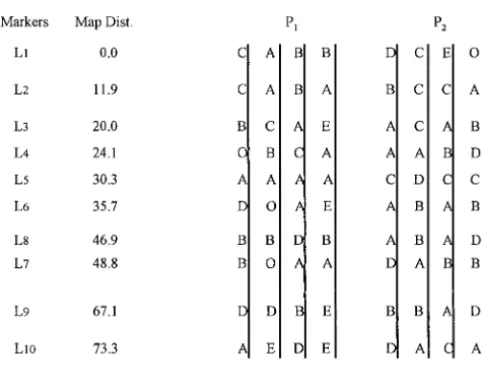
gested byCrosby(1973) was extended to simulate ge- genotypes at these marker loci and the recombination

frequencies between the adjacent loci are shown in Ta-netic recombination between linked loci. Chiasmata

interference, sexual differentiation in recombination ble 4. It should be noted that the alleles listed in the

same column for loci on the same chromosome have frequency, and segregation distortion were assumed to

be absent in the simulation model. the same linkage phase. The phenotypes of the two

parents and 200 offspring (a realistic number for actual A full-sib family was simulated by crossing two

tetra-ploid parental lines. Twenty-two codominant marker experiments) were scored at all 22 marker loci. To

eluci-date statistical properties, some pairs of these loci were loci were generated, 10 linked on the first chromosome,

5 on each of the second and third chromosomes, and studied in 100 repeated simulation trials.

Analysis of the simulated data:The genotypes of the 2 isolated loci that were independent of the rest. The

simulated parental genotypes at each of the marker loci two parents were predicted for each of the loci using

the method proposed byLuoet al.(2000), on the basis

were determined by sampling independently from six

possible alleles whose population frequencies were as- of the phenotypes of the parents and their offspring.

The predicted parental genotypes are tabulated in Table

sumed to be 0.3 (alleleA), 0.2 (alleleB), 0.2 (alleleC),

0.1 (allele D), 0.1 (allele E), and 0.1 (null allele O), 4 together with the corresponding probabilities. It can

be seen that the parental genotypes at 18 of the 22 respectively. Loci with more than six alleles were not

simulated, as these appear to be rare in practice (R. C. marker loci were diagnosed correctly with a prediction

probability of nearly 1.0. However, there were two

al-Meyer,personal communication). The main purpose

for choosing parental genotypes in such a way is to test most equally likely parental genotypes predicted for the

marker lociL2,L5,L20, andL22. For locusL2the parental

TABLE 4

The simulated parental genotypes (G1andG2), their corresponding phenotypes (P1andP2), and the most

likely parental genotypes (Gˆ1⫻Gˆ2) predicted at 22 simulated marker loci

Loci Chr r G1 G2 P1 P2 Gˆ1⫻Gˆ2(prob)

L1 1 0.00 CABB DCEO 11100000 00111000 ABBC⫻CDEO(1.0000)

L2 1 0.10 CABA BCCA 11100000 11100000 AABC⫻ABCC(0.4999) or

ABCC⫻AABC(0.4999)

L3 1 0.10 BCAE ACAB 11101000 11100000 ABCE⫻AABC(0.9999)

L4 1 0.05 OBCA AABD 11100000 11010000 ABCO⫻AABD(1.0000)

L5 1 0.10 AAAO CDCC 10000000 00110000 AAAO⫻CCCD(0.5000) or

AAAA⫻CCCD(0.5000)

L6 1 0.05 DOAE ABAB 10011000 11000000 ADEO⫻AABB(0.9999)

L7 1 0.10 BOAA DABB 11000000 11010000 AABO⫻ABBD(0.9989)

L8 1 0.05 BBDB ABAD 01010000 11010000 BBBD⫻AABD(0.9999)

L9 1 0.10 DDBE BBAD 01011000 11010000 BDDE⫻ABBD(0.9999)

L10 1 0.05 AEDE DACA 10011000 10110000 ADEE⫻AACD(1.0000)

L11 2 0.50 AACB ACDD 11100000 10110000 AABC⫻ACDD(1.0000)

L12 3 0.50 ACBB ACAA 11100000 10100000 ABBC⫻AAAC(0.9999)

L13 4 0.50 AOCA AEEB 10100000 11001000 AACO⫻ABEE(0.9999)

L14 4 0.10 BEBD ABCC 01011000 11100000 BBDE⫻ABCC(1.0000)

L15 4 0.10 BOBA AOCA 11000000 10100000 ABBO⫻AACO(0.9998)

L16 4 0.10 DCCA BOAD 10110000 11010000 ACCD⫻ABDO(1.0000)

L17 4 0.10 OBEA BCDC 11001000 01110000 ABEO⫻BCCD(1.0000)

L18 5 0.50 DCBC CDDO 01110000 00110000 BCCD⫻CDDO(0.9881)

L19 5 0.20 AOOE CCOB 10001000 01100000 AOOE⫻BCCO(1.0000)

L20 5 0.20 AAAC ADAC 10100000 10110000 AAAC⫻AACD(0.4988) or

AAAC⫻ACDO(0.4988)

L21 5 0.20 ODBB BCAE 01010000 11101000 BBDO⫻ABCE(1.0000)

L22 5 0.20 AADA ABAC 11010000 11100000 AAAD⫻AABC(0.4999) or

AAAD⫻ABCO(0.4900)

Chr, the linkage group number, andr, the recombination frequencies between adjacent loci, are the most likely predicted parental genotypes.

phenotypes are the same (1110000), but the most likely

parental genotypes are different (AABCandABCC) and

it is not possible at this stage to tell which parent has which genotype. Both genotypes at this locus were used in the linkage analysis. For the other three loci, allele

Ais present for all offspring, and this is consistent with

more than one configuration with multiple dosages of

A.The dosages of the informative alleles are the same

for the two possible configurations forL5,L20, andL22,

and so estimates of recombination frequencies are the same for the two configurations.

Pearson’s chi-square tests of independence were per-formed for all possible pairs of these marker loci using the test statistic given in Equation 1. Figure 2 displays the significance probabilities, transformed to distances as described previously, as dendrograms calculated us-ing nearest-neighbor cluster analysis and average link-age cluster analysis. The nearest-neighbor analysis shows

the three clusters (lociL1–L10,L13–L17, andL18–L22) have

each grouped at a distance of zero. LociL11 and L12

remained isolated until the distance exceeded 0.13.

However, the three linkage groups also merge at a very _{Figure2.—Cluster analysis of the 22 simulated loci, using}

small distance. Inspection of the significance levels _{(a) nearest-neighbor cluster analysis and (b) average linkage}

cluster analysis.

TABLE 5

The maximum-likelihood estimates of pairwise recombination frequencies (the upper diagonal) and the LOD scores (the second rows of the lower diagonal) calculated

for the most likely parental phases for lociL1–L10

Loci L1 L2 L2⬘ L3 L4 L5 L6 L7 L8 L9 L10

L1 — 0.11 0.18 0.19 0.18 0.23 0.24 0.33 0.36 0.40 0.39

L2 0.000 — — 0.13 0.10 0.13 0.22 0.30 0.34 0.35 0.33

31.03 — —

L2⬘ 0.000 — — 0.22 0.13 0.19 0.27 0.29 0.32 0.37 0.36

19.67 — —

L3 0.000 0.000 0.000 — 0.04 0.08 0.15 0.31 0.18 0.33 0.35

24.00 11.28 7.28

L4 0.000 0.000 0.000 0.000 — 0.03 0.09 0.16 0.21 0.28 0.28

35.55 24.59 17.86 47.82

L5 0.000 0.000 0.000 0.000 0.000 — 0.02 0.18 0.11 0.22 0.37

8.30 4.10 4.13 14.16 9.52

L6 0.000 0.000 0.000 0.000 0.000 0.000 — 0.11 0.09 0.24 0.26

18.33 7.16 5.13 37.57 33.91 12.38

L7 0.012 0.001 0.001 0.406 0.000 0.000 0.000 — 0.04 0.16 0.20

7.22 4.00 3.71 3.21 11.44 6.97 16.35

L8 0.013 0.461 0.461 0.000 0.000 0.000 0.000 0.000 — 0.17 0.20

2.96 0.97 1.43 7.48 14.13 7.99 14.20 11.29

L9 0.735 0.349 0.349 0.021 0.000 0.090 0.000 0.000 0.000 — 0.06

2.70 1.96 1.32 6.50 10.84 2.21 15.63 10.45 7.76

L10 0.418 0.000 0.000 0.013 0.000 0.410 0.000 0.000 0.000 0.000 —

3.44 4.16 2.89 3.19 8.71 0.66 9.96 11.08 6.59 56.26

Listed in the first rows of the lower diagonal are the significance of the independent tests.

association betweenL1andL18. Inspection of the aver- (e.g.,L1,L8) had large recombination frequencies and

lower LODs. age linkage cluster analysis shows that the same initial

groupings form more slowly, but that locusL18is clearly The maximum-likelihood estimates of the pairwise

recombination frequencies and the LOD scores in Table

associated with L19 and L20, and the average distance

between locusL18and lociL1–L10is large. The distantly 5 were used to construct a linkage map of these genetic

marker loci using the JoinMap linkage software (Stam

linked groupL18–L22finally merges at a large distance

using average linkage cluster analysis, but inspection of andVan Ooijen1995), as summarized in Figure 3. The

best-fitted map predicted from JoinMap indicates that the significance levels shows highly significant

associa-tions between 6 of the 10 pairs of this group, and we lociL1–L10were joined into a correct order except that

the relative simulated positions of the marker loci L7

proceed assuming that they form a linkage group.

Linkage analysis was performed on all pairs of loci andL8were reversed. The map distances of the linkage

group agreed well with the actual ones. within each linkage group. For brevity only the results

from the largest linkage group (loci L1–L10) are pre- The linkage phases of the parental genotypes were

reconstructed using the procedure described in the sented. Table 5 shows the significance of this test (the

first rows of the lower diagonal), the maximum-likeli- above analysis. Table 6 illustrates the parental linkage

phases at every pair of loci with a differencedij ⬎3 in

hood estimates of recombination frequencies (the

up-per diagonal) for the most likely phase, and the corre- the log-likelihood between the most likely and second

most likely phase. Locus L5does not appear in Table

sponding LOD scores (the second rows of the lower

diagonal) among the pairs of loci. It can be seen that 6, as there was only one phase with a recombination

frequency⬍0.5 in each case. The reconstructed linkage

the true parental genotype atL2has consistently higher

LOD scores in its pairings with L1,L3, L4,L6, and L7 phases of the parental genotypes are shown in Figure

3. This reconstruction uses the most likely phase for all

(i.e., all the highly significant linkages) than the other

predicted parental genotype (L2⬘) with the parental ge- pairs except for four [(L1,L8), (L1,L9), (L2, L7), (L6,

L9)]. For these four pairs, the largest difference in the

notypes reversed. The estimate of the recombination

frequency and LOD score were unaffected by the choice log-likelihood between the most likely phase and the

reconstructed phase was 0.56, and the difference in

between the alternative genotypes for locus L5. Most

cases where the independence test was significant (P⬍ the estimates of the recombination frequency was always

⬍0.01. The reconstructed phase is identical to that

simu-0.05) corresponded to LOD scores⬎3, although a small

TABLE 6

The most likely parental genotypic linkage phases (S1andS2)

and the difference (dij) in log-likelihood value between

the most likely and the second most likely linkage phases of the marker lociLiandLj

Li Lj S1 S2 dij

1 2 CC/AA/BB/BA DB/CC/EC/OA 10.18 1 3 CB/AC/BA/BE DA/CC/EA/OB 15.19 1 4 CO/AB/BC/BA DA/CA/EB/OD 7.72 1 6 CD/AO/BA/BE DA/CB/EA/OB 4.32 2 3 CB/AC/BA/AE BA/CC/CA/AB 4.37 3 4 BO/CB/AC/EA AA/CA/AB/BD 18.72 3 6 BD/CO/AA/EE AA/CB/AA/BB 4.19 3 8 BB/CB/AD/EB AA/CB/AA/BD 3.51 4 6 OD/BO/CA/AE AA/AB/BA/DB 11.67

4 8 OB/BB/CD/AB AA/AB/BA/DD 8.87

4 9 OD/BD/CB/AE AB/AB/BA/DD 3.95

Figure3.—The best-fitted map, the estimated map distance _{4 10 OA/BE/CD/AE AD/AA/BC/DA 3.49}

(in centimorgans), and parental linkage phases reconstructed _{7 8 BB/OB/AD/AB DA/AB/BA/BD 4.32} from the codominant marker lociL1–L10from the simulation _{8 9 BD/BD/DB/BE AB/BB/AA/DD 3.65}

study.

9 10 DA/DE/BD/EE BD/BA/AC/DA 14.64

Linkage maps of loci L13–L17and L18–L22 were

esti-mated using the same approach. In each case the order due to the selection of the most likely phase. The

paren-and phase were reconstructed correctly. tal linkage phases at the marker loci were correctly

pre-To investigate the reliability of the pairwise linkage dicted for at least 89% of simulations with cases with

phase estimation, separate simulation trials were per- rⱕ0.3.

formed. The simulated recombination frequencies were 0.05, 0.1, and 0.3 and the sample size was 200. Figure

LINKAGE ANALYSIS OF EXPERIMENTAL DATA IN

4 illustrates the maximum-likelihood estimate of r

be-AUTOTETRAPLOID POTATO

tweenL9andL10(Figure 4a), and betweenL7andL10

(Figure 4b), and the corresponding LOD scores calcu- Some preliminary data from the Scottish Crop

Re-search Institute were used to test this approach, using lated at all possible parental linkage phase

configura-tions. It can be seen that the correct parental linkage five SSR marker loci (STM0017, STM1017, STM1051,

STM1052, and STM1102) and six AFLP marker loci

phases were the most likely when the marker loci were

closely linked (i.e.,rⱕ0.1), although the difference in (e35m61–18,e35m61–21,e37m39–14,e39m61–7,e46m37–

12, andp46m37–12) scored on 77 offspring from a cross

the likelihood value between the most likely and the

second most likely linkage phases reduced as the value between two parental lines: the advanced potato

breed-ing line 12601abl and the cultivar Stirlbreed-ing (Bradshaw

ofrincreased. When the loci were loosely linked (i.e.,

r⫽ 0.3), the most likely parental linkage phase could et al.1998). Details of scoring the DNA molecular

mark-ers are described inMeyeret al.(1998) andMilbourne

differ from the simulated phase, but when this occurred

the MLE of r at the most likely phase was always very et al.(1998). Preliminary analysis of the AFLP markers

(Meyeret al.1998), and of the SSR markers in diploid close to that calculated at the simulated phase.

Further simulations were carried out to examine the and tetraploid populations (Milbourneet al.1998)

sug-gested that these markers are all on the same linkage power to detect linkage and the bias in estimates of the

recombination frequency. Table 7 shows the means and group.

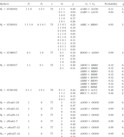
Table 8 summarizes the parental phenotypes and the standard deviations of the maximum-likelihood

esti-mates of recombination frequencies for 100 replicate phenotype distribution of the offspring at the marker

loci. Of a total of 77 offspring scored at these marker simulations of some pairs of marker loci considered

above. Linkage was detected as significant (P ⬍ 0.05) loci, there were 73, 73, 72, and 70 progeny whose

pheno-types at the marker lociSTM1017,STM1051,STM1052,

by both the independence test and the likelihood-ratio

test with a frequency ⱖ90% when the recombination and STM1102, respectively, were unambiguously

ob-served. The phenotypic data were used to predict the

frequencyrⱕ0.3, except for the least informative pair

(L2,L5). Forr ⫽0.5, the frequency of significant tests parental genotypes using the method of Luo et al.

(2000). The predicted parental genotypes at the marker

was close to 5%. The means of the MLEs ofrwere close

to the corresponding simulated values forrⱕ0.3. For loci are also shown in Table 8 together with the

corre-sponding prediction probabilities and the␹2_{values of}

Figure4.—The maximum-likelihood estimates of recombination frequencies and the corresponding LOD scores for all possible linkage phases for (a) lociL9andL10and (b) lociL7andL10. Arrows indicate the true linkage phases.

the goodness-of-fit test. It was found from the analysis linkage analysis. The maximum-likelihood estimates of

recombination frequency between the pairs of marker that the number of possible genotype configurations

with probabilityⱖ0.1 varies from 1 (atSTM0017,STM1051, loci are listed on the upper diagonal and the LOD scores

are given in the second rows of the lower diagonal of

and the AFLP marker loci) up to 8 (STM1017). For this

locus, all that can be deduced is that allele 1 occurs in Table 9. Both possible genotypes for locusSTM1052 are

shown, as these gave slightly different estimates of the a simplex condition in parent 1.

The independence tests were performed for all possi- recombination frequencies and LOD scores. The

likeli-hood for genotype AABO ⫻ AACO was always larger

ble pairs of the marker loci and the significance

proba-bilities of the tests are listed as the first rows of the lower than for the other genotype. The use of the alternative

parental genotypes at lociSTM1017 andSTM1102 did

diagonal in Table 9, along with the results of a pairwise

TABLE 7

Mean and standard deviation of the maximum-likelihood estimate of recombination frequency and the empirical statistical power for detecting the linkage based on 100 simulations

Set Marker loci n r rˆ⫾SD RI ␤1 ␤2 ␰

1 L1andL2 100 0.1 0.0969⫾0.030 0.95 99 99 99

2 L1andL2 200 0.1 0.1051⫾0.021 0.95 100 100 100

3 L1andL2 200 0.3 0.3027⫾0.042 0.80 100 95 93

4 L1andL2 200 0.5 0.4197⫾0.029 0.74 6 4 —

5 L1andL3 100 0.1 0.1012⫾0.022 1.65 99 99 99

6 L1andL3 200 0.1 0.1002⫾0.015 1.65 100 100 100

7 L1andL3 200 0.3 0.3030⫾0.029 1.31 100 100 100

8 L1andL3 200 0.5 0.4473⫾0.018 1.15 5 4 —

9 L2andL5 100 0.1 0.1053⫾0.094 0.10 100 75 100

10 L2andL5 200 0.1 0.1060⫾0.069 0.10 100 97 100

11 L2andL5 200 0.3 0.3057⫾0.088 0.11 79 55 89

12 L2andL5 200 0.5 0.4062⫾0.047 0.12 2 0 —

13 L9andL10 100 0.1 0.1033⫾0.029 1.34 100 100 100

14 L9andL10 200 0.1 0.1000⫾0.018 1.34 100 100 100

15 L9andL10 200 0.3 0.2948⫾0.030 1.36 100 100 89

16 L9andL10 200 0.5 0.4409⫾0.025 1.37 3 1 —

RI, the relative information;␤1, the frequency of the significant tests of independence at␣ ⫽0.05;␤2, the

TABLE 8

Phenotypes of five SSR and six AFLP marker loci scored on two parents (P1, Stirling;P2, 12601abl) and

their progeny and the predicted parental genotypesG1andG2at these marker loci

Markers P1 P2 n Oi fi G1⫻G2 Probability ␹2d.f.

M1⫽STM1052 1 1 0 1 0 1 72 1 1 1 0.28 AABO⫻ACOO 0.11 5.88

0 1 1 0.04 AABO⫻AACO 0.84 3.56 1 0 0 0.25

1 1 0 0.17 1 0 1 0.26

M2⫽STM1051 1 1 1 0 0 1 0 1 73 1 1 0 1 0.23 ABBC⫻BBDO 0.95 5.90

1 1 0 0 0.16 0 1 0 0 0.04 1 1 1 0 0.05 0 1 1 0 0.19 0 1 0 1 0.11 0 1 1 1 0.12 1 0 1 1 0.03 1 1 1 1 0.05

M3⫽STM0017 0 1 1 0 77 0 1 0.18 BOOO⫻AOOO 0.99 4.82

0 0 0.25 1 1 0.35 1 0 0.22

M4⫽STM1017 1 1 0 1 73 1 1 0.49 ABOO⫻BBBO 0.12 0.01

0 1 0.51 ABOO⫻BBBB 0.12 0.01

ABBO⫻BBBO 0.12 0.01

ABBO⫻BBBB 0.12 0.01

ABBB⫻BOOO 0.12 0.01

ABBB⫻BBOO 0.12 0.01

ABBB⫻BBBO 0.12 0.01

ABBB⫻BBBB 0.12 0.01

M5⫽STM1102 0 1 1 1 0 1 70 0 1 1 0.44 BBCO⫻ACCC 0.46 2.55

1 1 1 0.36 BBCC⫻ACCC 0.46 2.55 1 0 1 0.13

0 0 1 0.07

M6⫽e35m61–18 1 0 77 1 0.53 AOOO⫻OOOO 0.99 0.32

0 0.47

M7⫽e35m61–21 1 0 77 1 0.84 AAOO⫻OOOO 0.99 0.06

0 0.16

M8⫽e37m39–14 1 0 77 1 0.62 AOOO⫻OOOO 0.99 4.69

0 0.38

M9⫽e39m61–7 1 0 77 1 0.51 AOOO⫻OOOO 0.99 0.05

0 0.49

M10⫽e46m37–12 1 0 77 1 0.45 AOOO⫻OOOO 0.99 0.01

0 0.55

M11⫽p46m37–12 1 0 77 1 0.48 AOOO⫻OOOO 0.99 0.00

0 0.52

Oiandfiare marker phenotypic classes of the offspring and the corresponding frequencies, respectively.

not affect the estimates of recombination frequencies reconstructed phases are illustrated in Figure 5. For loci

STM1017 and STM1102, the dosage of the alleles that

and LOD scores.

The MLEs of the pairwise recombination frequencies are present for all offspring is uncertain, but the phase

of the segregating alleles can be reconstructed. For and the LOD scores were used to map the marker loci

using JoinMap. The 11 markers were mapped as a link- STM0017, there is uncertainty about the phase for

par-ent 2 as this marker is well separated from the other SSR age group with a length of 48.9 cM (using genotype

AABO⫻AACOforSTM1052). The order was the same markers that are informative about parent 2, although

alleleAof this marker is unlikely to be linked in coupling

using the alternative genotype, and the calculated

length in this case was 48.7 cM. The allelic linkage to the simplex alleles of the other SSR markers (Afor

STM1102, C for STM1052, and D for STM1051). The

phases of the parental genotypes at the marker loci were

TABLE 9

The maximum-likelihood estimates of pairwise recombination frequencies (the upper diagonal) among five SSR and six AFLP marker loci in autotetraploid potato, their corresponding LOD scores (the second rows of the lower diagonal),

and the significance level of the independence tests (the first rows of the lower diagonal)

Loci M1 M1⬘ M2 M3 M4 M5 M6 M7 M8 M9 M10 M11

M1 — – 0.028 0.166 0.041 0.003 0.156 0.003 0.111 0.072 0.248 0.012

M1⬘ — — 0.028 0.201 0.017 0.004 0.084 0.002 0.111 0.029 0.224 0.097

M2 0.000 0.000 — 0.196 0.105 0.121 0.239 0.110 0.164 0.143 0.285 0.123

35.08 34.60

M3 0.109 0.109 0.014 — 0.274 0.391 0.026 0.150 0.399 0.053 0.104 0.065

1.75 1.59 2.49

M4 0.017 0.017 0.033 0.001 — 0.499 0.274 0.371 0.270 0.278 0.329 0.352

1.58 1.64 2.94 3.36

M5 0.003 0.003 0.017 0.115 0.375 — 0.413 0.208 0.153 0.466 0.398 0.136

5.50 4.98 4.84 0.90 0.00

M6 0.086 0.086 0.114 0.000 0.000 0.407 — 0.074 0.399 0.053 0.104 0.065

0.89 1.08 1.32 19.15 3.36 0.10

M7 0.015 0.015 0.009 0.006 0.351 0.000 0.001 — 0.110 0.178 0.107 0.078

3.54 3.38 3.28 1.77 0.19 2.42 2.82

M8 0.000 0.000 0.000 0.120 0.197 0.005 0.463 0.000 — 0.299 0.175 0.100

10.77 10.77 7.81 0.07 0.36 2.19 0.07 2.69

M9 0.075 0.075 0.036 0.000 0.000 0.721 0.000 0.017 0.211 — 0.079 0.228

1.37 1.47 2.58 16.07 3.20 0.01 16.07 1.32 0.29

M10 0.172 0.172 0.063 0.000 0.003 0.371 0.000 0.005 0.071 0.000 — 0.213

0.49 0.49 0.87 12.02 1.90 0.14 12.02 1.95 0.82 13.76

M11 0.007 0.007 0.000 0.054 0.407 0.019 0.001 0.001 0.017 0.110 0.080 —

2.92 2.82 10.14 1.51 0.15 2.10 1.51 2.67 1.26 0.56 0.64

The order of the marker loci is in accordance with that listed in Table 8.M1andM1⬘represent the two alternative genotypes

at locusSTM1052.

and the most likely phase is for the pairSTM0017 and frequency and the LOD score for all possible phases.

STM1102, for which the inferred phase has a log-likeli- The EM algorithm allows this to be done for any

hood 1.16 less than the most likely, although both parental genotype configuration.

phases correspond to loose linkages (recombination fre- 5. For each pair, identify the phase with the largest

quency≈0.4, LOD 0.90). The conclusion that the SSR likelihood and estimate the difference in

log-likeli-markers form a single linkage group agrees with the hood dij between the most likely and second most

analysis of these markers in a diploid cross (Milbourne likely phase.

et al.1998). 6. Use the recombination frequencies and LOD scores

for the most likely phases to order the loci and calculate distances between them.

DISCUSSION _{7. Reconstruct the linkage phase for the complete}

link-age group, using pairs in order of decreasingdij.

In this article we have developed the methodology for

8. Check that the inferred linkage phases are the most

constructing linkage maps of codominant or dominant

likely ones for all pairs with a substantial difference genetic markers in autotetraploid species under

chro-in log-likelihood, for exampledij⬎ 3.

mosomal segregation,i.e., the random pairing of four

9. For pairs where the inferred phase is not the most

homologous chromosomes to give two bivalents. Our

likely phase, compare estimates of the recombina-strategy has the following steps:

tion frequencies and LOD scores. Recalculate the

1. Identify which parental genotype(s) are consistent _{linkage map on the basis of the inferred phase if}

with the parental and offspring phenotype data. _necessary.

2. For each pair of loci, calculate Pearson’s chi-square

In the simulated and experimental data sets, there statistic for independent segregation, and its

sig-have been examples of loci for which more than one nificance.

genotype for the parents is possible. This occurred for

3. Use cluster analysis, based on the significance, to

three reasons. First, some alleles may be present in all partition the loci into linkage groups. For each

link-offspring, and so are uninformative, for example, simu-age group in turn, proceed as follows: