Quadratic Surface Support Vector Machines with Applications.

(1)

ABSTRACT

LUO, JIAN. Quadratic Surface Support Vector Machines with Applications. (Under the direction of Shu-Cherng Fang.)

(2)

(3)

Quadratic Surface Support Vector Machines with Applications

by Jian Luo

A dissertation submitted to the Graduate Faculty of North Carolina State University

in partial fulfillment of the requirements for the Degree of

Doctor of Philosophy

Industrial Engineering

Raleigh, North Carolina 2014

APPROVED BY:

Russell E. King Yahya Fathi

Yunan Liu Shu-Cherng Fang

(4)

DEDICATION

This dissertation is dedicated to my family for their endless love and support: Nenghui Luo, my dear Dad

(5)

BIOGRAPHY

(6)

ACKNOWLEDGEMENTS

I would like to express my deepest and sincerest gratitude to Dr. Shu-Cherng Fang for guiding me through the Ph.D. study at North Carolina State University. His wisdom, knowledge, personality, patience, and professional guidance were invaluable to me.

I am also thankful to Dr. Russell E. King, Dr. Yahya Fathi and Dr. Yunan Liu for offering valuable comments and suggestions as my committee members. Special thanks to the graduate school representative Dr. Kazufumi Ito for his help in my defense. I am also deeply obliged to Dr. John E. Lavery and Dr. Yanqin Bai for their stimulating advices and kind help in my graduate study.

Thanks to the staff of Industrial and Systems Engineering Department, especially Mrs. Cecilia Chen, Mr. Bill Irwin, Mr. Justin Lancaster and Mr. Hakan Sungur, for their supports and help.

(7)

LIST OF TABLES

Table 5.1 Descriptions of Real-world Data Sets . . . 53

Table 5.2 Memory Requirements for All Models . . . 55

Table 5.3 Artificial Data Test . . . 56

Table 5.4 Iris Data Test . . . 57

Table 5.5 Car Evaluation Data Test . . . 58

Table 5.6 Wisconsin Breast Cancer Data Test . . . 59

Table 5.7 Skin Data Test . . . 60

Table 5.8 Artificial training data set with p% outliers . . . 61

Table 5.9 Artificial Data Test . . . 62

Table 5.10 Iris Data Test . . . 63

Table 5.11 Car Evaluation Data Test . . . 64

Table 5.12 Wisconsin Breast Cancer Data Test . . . 65

Table 5.13 Skin Data Test . . . 66

Table 5.14 Artificial training data set with p% outliers . . . 67

Table 6.1 Multi-classed Data Sets . . . 71

Table 6.2 Iris Data Test in Three Classes . . . 72

Table 6.3 Balance Data Test in Three Classes . . . 73

Table 6.4 Credit Data Sets . . . 77

Table 6.5 German Credit Data Test . . . 78

Table 6.6 Australian Credit Data Test . . . 79

Table 6.7 Iris Data Test in Three Classes . . . 88

(10)

LIST OF FIGURES

Figure 1.1 A SVM Classifier (an image from [26]) . . . 2

Figure 1.2 A Soft SVM Classifier . . . 3

Figure 1.3 A Soft SVM with Kernel Classifier . . . 4

Figure 1.4 Face Detection Based on SVM (an image from [76]) . . . 5

Figure 1.5 A Kernel-free Nonlinear SVM Model . . . 6

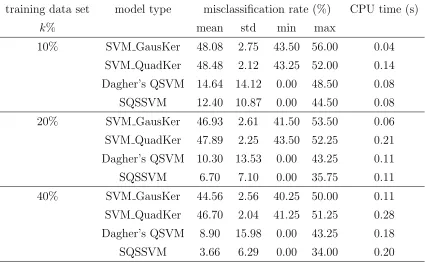
Figure 2.1 The Separating Line . . . 12

Figure 2.2 Fisher Discriminant Analysis . . . 17

Figure 3.1 The Separating Quadratic Curve . . . 24

Figure 4.1 Artificial Data with a Nonconvex Separating Quadratic Curve . . . . 37

Figure 4.2 Affinity Among Training Points . . . 39

Figure 4.3 Fuzzy Memberships of Training Points . . . 40

Figure 5.1 A Second Type Artificial Data Set . . . 53

Figure 5.2 Iris Data . . . 54

Figure 5.3 Skin Data . . . 54

Figure 6.1 Clustering Analysis . . . 80

(11)

Chapter 1 INTRODUCTION

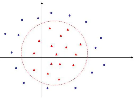
Binary classification is an important task in information extraction from data. Support vector machines (SVM) are effective and commonly used classification techniques. As an optimization-based binary classification technique, SVM models are first proposed around 1995 [26, 112]. The basic concept of SVM models is to find a hyperplane that separates the training points into two classes, with a maximum level of separation [113]. The aim of this dissertation is to propose some quadratic surface support vector machine (QSSVM) models for binary classification directly using a quadratic function instead of using a hyperplane. In this dissertation, we first propose a soft QSSVM model and two fuzzy QSSVM models. Then we study the properties of the proposed QSSVM models and conduct computational experiments to investigate their performance. Finally we extend the proposed QSSVM models for multi-class classification, credit scoring and cluster analysis.

1.1 Historic Background of Support Vector Machines

(12)

Figure 1.1: A SVM Classifier (an image from [26])

Based on the statistical learning theory and structural risk minimization principal, SVM models had been proposed and largely developed at AT&T Bell Laboratories by Vapnik and co-workers [26, 83, 112]. Due to the industrial requirements, SVM research had a sound orientation towards real-world applications. The initial application of SVM models focused on OCR (optical character recognition). Within a short period of time, SVM classifiers became competitive with the best available systems for OCR and object recognition tasks [84, 85]. A comprehensive tutorial on SVM classifiers was published in [16]. Moreover, in the applications of regression and time series prediction, excellent performances were rapidly obtained [34, 94]. A snapshot of the state of the art of SVM models can be seen in [86]. SVM has evolved into an active research area from 2000.

1.2 Statement of Problems

For binary classification, a training data set ofn records{(ˆx1_,_y_ˆ1_),_{· · ·} _,_(ˆ_xi_,_y_ˆi_),_{· · ·} _,_(ˆ_xn_,

ˆ

yn₎_}_{is given, where}_ˆ_xi _{= [ˆ}_xi

1,xˆi2,· · · ,xˆim]T ∈Rmindicates the position of thei-th training

point in the m-dimensional space, and the label ˆyi _{= +1 or} ₋_{1 indicates that point} _x_ˆi

belongs to Class C1 or Class C2, respectively. A natural idea is to identify a boundary

that separates the training points in Class C1 from those in Class C2. For the simple

example of training points in two-dimensional space shown in Figure 1.1, all red circle points with their labels ˆyi = +1 belong to Class C1 while all black circle points with

(13)

Figure 1.2: A Soft SVM Classifier

1.1) that breaks the training points into the two classes accordingly.

If the n training points {ˆx1,· · · ,xˆi,· · · ,ˆxn} are separable by a hyperplane, then the SVM model [26, 112] is used to find the parameter vector (u, d)∈_Rm+1 _{of a hyperplane}

f(x)≡uTx+d= 0

that separates all training points into Class C1 or Class C2 according to their respective

labels, with a maximum level of separation (see Figure 1.1). Equivalently, the parameter vector (u, d)∈_Rm+1 _{is to be found such that, for each} _i_{= 1,}_{· · ·} _{, n,}

(

uTxˆi+d≥+1, for ˆyi = +1, uTxˆi+d≤ −1, for ˆyi =−1.

In Figure 1.1, after applying the SVM model, the black solid separating line is obtained. For real-world binary classification applications, the obtained training data set is often contaminated with outliers and noises (see Figure 1.2). In these situations, it is possible that no hyperplane can separate all training points into their corresponding classes correctly. To handle this case, a soft SVM model was developed using a continuous measure of misclassification error [26] so that the black separating line in Figure 1.2 is obtained.

However, the soft SVM model does not work well when most points in the training data set are not separable by a hyperplane in the m-dimensional space [29, 113]. Take a simple example shown on the left of Figure 1.3, all blue training points with their labels ˆyi _{= +1 belong to Class} _C

1 while all red training points with their labels ˆyi =−1

belong to Class C2. We can see that the training points are not separable by a line, but

separable by a circle. To overcome this difficulty indirectly, each training pointˆxi _∈

Rmis

first mapped into a corresponding pointφ(ˆxi₎_∈

(14)

Figure 1.3: A Soft SVM with Kernel Classifier

function φ(x) :_Rm _→

Rl. Then, in the l-dimensional space, a soft SVM model with the

kernel [88, 113] is used to seek a hyperplane that separates all mapped training points

{φ(ˆx1_),_{· · ·} _{, φ(ˆ}_xi_),_{· · ·} _{, φ(ˆ}_xn₎_}_{into Class} _C

1 or Class C2 according to their labels, with a

maximum level of separation. In Figure 1.3, the training points in the two-dimensional space are first mapped into the three-dimensional space, using a nonlinear kernel function. Then a three-dimensional hyperplane (on the right of Figure 1.3) can be found to separate the mapped training points into two classes according to their respective labels.

As a commonly-used machine learning technique [104, 112, 113], soft SVM models with kernels have achieved great success in many real-world applications. One example of applying the soft SVM models with kernels to the face detection [76] is shown in Figure 1.4, where circles represent face patterns and squares represent non-face patterns. Also the face and non-face patterns near the separating curve are shown in Figure 1.4. We can see that some of non-face patterns are very similar to the face patterns.

1.3 Motivations

(15)

Figure 1.4: Face Detection Based on SVM (an image from [76])

these two concerns, in this dissertation, we propose some kernel-free nonlinear SVM models which classify the data set directly using a quadratic function for separation.

The proposed kernel-free nonlinear SVM models find the parameter set (W,b, c) of a quadratic surface

g(x)≡ 1

2x

T_W_x₊_bT_x₊_c_{= 0,}

whereW =WT =      

w11 w12 · · · w1m

w12 w22 · · · w2m

.. .

w1m w2m · · · wmm

     

∈_Rm×m_, _b₌

     

b1

b2

.. . bm

     

∈_Rm _and _c_∈

R,

that separates the n training points {ˆx1_,_{· · ·}_,_x_ˆi_,_{· · ·} _,_ˆ_xn_} _{into Class} _C

1 or Class C2

(16)

Figure 1.5: A Kernel-free Nonlinear SVM Model

convex or nonconvex. Using a simple classification problem in Figure 1.5 as an example, we plan to propose a kernel-free nonlinear SVM model for directly finding the parameters of the red circle, which separates all training points according to their respective labels.

For real-world binary classification applications, the available training data set is often corrupted with noise. Some points in the training data set may even be misplaced in the wrong class by accident. These points are known as outliers. To deal with these outliers and noise, along with incorporating a continuous measure of misclassification error similar to the soft SVM model, we plan to enhance the capability of the proposed kernel-free nonlinear SVM model using the concept of fuzziness, which is characterized by figuring out the relative importance of each training point.

(17)

1.4 Outline

(18)

Chapter 2 LITERATURE REVIEW

In this chapter, we first review some data classification methods. Related ideas of soft and fuzzy support vector machine (SVM) models for binary classification using a hy-perplane for separation are then reviewed and discussed. Moreover, we review the linear Fisher discriminant analysis (FDA), quadratic FDA and linearly constrained quadratic Programming (LCQP) problems. The ideas of decomposition programming are also in-troduced and discussed.

2.1 Data Classification Methods

(19)

SVM models.

A common approach for classifiers is to use decision trees to partition and segment known labeled records [115]. New records can be classified by traversing the tree from the root through branches and nodes, to a leaf representing a class. The path that a record takes through a decision tree can then be represented as a rule. One of the most significant advantages of decision trees is the fact that knowledge can be extracted and represented in the form of classification (if-then) rules. Decision trees are recognized as highly unstable classifiers with respect to minor perturbations in the training data [43].

The most interesting feature of BN [40, 43], compared to decision trees is the pos-sibility of taking into account prior information about a given problem and the simple structure lends itself to comprehensible visualizations. BN can readily handle incomplete data sets and allow one to learn about causal relationships. A major problem of BN classifiers is that they are not suitable for data sets with many features [23]. The reason is that trying to construct a very large network is not feasible in terms of time and space. KNN classifiers [27, 43] are based on learning by analogy. The training samples are described by n dimensional numeric attributes. Each sample represents a point in an n-dimensional space. In this way, all of the training samples are stored in an n-n-dimensional pattern space. Given an unknown sample, a k-nearest neighbor classifier searches the pattern space for the k training samples that are closest to the unknown sample. “Close-ness” is often defined in terms of Euclidean distance. The unknown sample is assigned to the most common class among its k nearest neighbors. The main advantage of the KNN method is the simplicity and no parametric assumptions, while the disadvantage of KNN method is that the time to find the nearest neighbor in a large training set is prohibitive [92].

The classifiers generated by NN [121] are described as complex mathematical func-tions, which are incomprehensible or opaque to humans. NN follows a discriminating rule to classify the data set. Powerful full-data fitting or function approximation makes NN susceptible to over-fitting. Combining several NN may improve their performances [43]. The opacity of NN limits them in many real-life applications where both accuracy and comprehensibility are required, e.g., medical diagnosis and credit risk evaluation [44].

(20)

from applications and extensive experimentation to the theory. The key features of SVM models are the absence of local minima, the sparseness of the solution, the use of kernels and the capacity control obtained by maximizing the margin [90]. Classical classifying and learning methods like NN suffer from their theoretical weakness, e.g., back-propagation NN or multilayer perceptron NN usually converges to a local optimal solution, while SVM models can provide a unique solution with some important properties of convexity [97].

2.2 Support Vector Machine Models

In this section, we first review some basic ideas of soft SVM models with kernels for binary classification using a hyperplane for separation. Then some variants and extensions of soft SVM models with kernels are introduced.

For binary classification, a training data set of n records {(ˆx1_,_y_ˆ1_),_{· · ·} _,_(ˆ_xi_,_y_ˆi_),_{· · ·} _,

(ˆxn_,_y_ˆn₎_} _{is given, where} _ˆ_xi _{= [ˆ}_xi

1,xˆi2,· · · ,xˆim]T ∈ Rm indicates the position of the i-th

training point in the m-dimensional space, and the label ˆyi _{= +1 or} ₋_{1 indicates that}

point ˆxi _{belongs to Class} _C

1 or Class C2, respectively.

The basic concept of the SVM model is to find the parameter vector (u, d) ∈ _Rm+1

of a hyperplane

f(x)≡uTx+d= 0 (1)

that separates the n training points {ˆx1_,_{· · ·} _,_x_ˆi_,_{· · ·} _,_x_ˆn_} _{into Class} _C

1 and Class C2,

with a maximum level of separation [113].

Definition 2.2.1([31]).Consider a training data set{(ˆx1_,_y_ˆ1_),_{· · ·} _,_(ˆ_xi_,_y_ˆi_),_{· · ·} _,_(ˆ_xn_,_y_ˆn₎_}_,

where xˆi _∈

Rm, yˆi ∈ {+1,−1}, i= 1,· · · , n. If there exists (eu,d)e ∈R

m+1 _{and a number}

> 0 such that, for any i with yˆi _{= +1}_{, we have}

e uT_ˆ_xi ₊

e

d ≥ , and, for any i with

ˆ

yi ₌ ₋₁_{, we have}

e uT_ˆ_xi₊

e

d ≤ −, then we say the training data set for classification is linearly separable.

Let us start with the linearly separable training data set. From Definition 2.2.1, for the n training points {ˆx1_,_{· · ·} _,_ˆ_xi_,_{· · ·} _,_x_ˆn_} _{in two classes, we know}

( e

uTˆxi+de≥, for ˆyi = +1

e

(21)

Letu = ue

, d=

e

d

, we have

(

uTˆxi+d≥1, for ˆyi = +1 uTˆxi+d≤ −1, for ˆyi =−1

This is equivalent to

( ˆ

yi(uTxˆi+d)≥1 ˆ

yi =±1 (2)

Definition 2.2.2 ([30]). Given a training point ˆxi _∈

Rm, its class label yˆi ∈ {+1,−1}

and a linear function f(x) = uT_x₊_d_{, where} _{(u, d)} _∈

Rm+1, we call βˆi = ˆyif(ˆxi) the

functional margin at point xˆi _{with respect to the hyperplane} _f_{(x) = 0}_.

Definition 2.2.3. Given a training point xˆi _∈

Rm, its class label yˆi ∈ {+1,−1} and

a linear function f(x) = uT_x₊_d_{, where} _{(u, d)} _∈

Rm+1, the vector ∇f(ˆxi) (= u) is

called the gradient direction at point xˆi _{with respect to the hyperplane} _{f(x) =} _f_(ˆ_xi₎_{. If}

ˆ

yi = +1 (or −1), the negative (or positive) gradient direction −u (or u) is called the related gradient direction at point ˆxi with respect to the hyperplane f(x) = f(ˆxi).

and a linear function f(x) =uT_x₊_d_{, where} _{(u, d)}_∈

Rm+1, the related gradient direction

at pointˆxi _{with respect to the hyperplane} _{f(x) =}_f_(ˆ_xi₎_{intercepts the hyperplane} _{f(x) = 0}

at a point ˆxB_{. The length of the segment} _ˆ_xi_ˆ_xB_{, denoted as} _β

i, is called the geometrical

margin at point ˆxi _{with respect to the hyperplane} _f_{(x) = 0}_.

Rm, its class label yˆi ∈ {+1,−1} and a

linear function f(x) = uTx+d, where (u, d) ∈ _Rm+1_{, the related gradient direction at}

point ˆxi with respect to the hyperplane f(x) =f(ˆxi) intercepts the hyperplanef(x) = +1

(or−1) at a pointˆxi. The length of the segmentˆxi_x_ˆB_{, denoted as}_β¯

i, is called the relative

geometrical margin at the point ˆxi _{with respect to the hyperplane} _f_{(x) = 0}_.

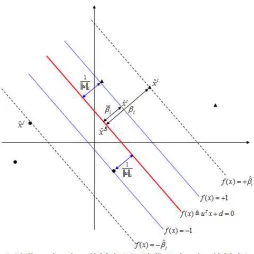
Figure 2.1 illustrates ˆxi_, _x_ˆi_, _x_ˆB_{, ˆ}_β

i, βi and ¯βi for m = 2. In this figure, the red line

is the separating line of the two classes. In Dagher’s paper [30], the relationship between the functional and geometrical margin at a training pointxˆi _{is given by}_β

i =

ˆ

βi

kuk2. Also,

(22)

Figure 2.1: The Separating Line

margin. Then, at pointˆxi, ¯βi =kˆxB−ˆxik2 = _k_u1_k

2. The objective of the SVM model then

be restated as “to maximize the sum of the relative geometrical margins at all training points with respect to a hyperplane f(x) = 0 subject to the condition that each training point has a no less than 1 functional margin”. (see Figure 2.1, where the distance between the two blue lines is maximized subject to the condition that no training point exists between the two blue lines.)

For a linearly separable training data set {(ˆx1_,_y_ˆ1_),_{· · ·} _,_(ˆ_xn_,_y_ˆn₎_}_{, we then consider}

the following optimization problem:

max n

kuk2

s.t. yˆi(uTˆxi+d)≥1, i= 1,2,· · · , n, (u, d)∈_Rm+1_.

(23)

SVM model becomes

min nkuk2₂

s.t. yˆi(uTˆxi+d)≥1, i= 1,2,· · · , n, (u, d)∈_Rm+1_.

This problem is equivalent to the following optimization problem [12]:

min 1

2kuk

2 2

s.t. yˆi(uTˆxi+d)≥1, i= 1,2,· · · , n, (SVM) (u, d)∈_Rm+1_.

However, the training data set is not linearly separable in general. Different slack tech-niques are used to relax the constraints in the model (SVM) for developing soft SVM models [26]. The commonly used soft SVM model is to add a slack variable ξi ≥ 0 for

each constraint in the model (SVM) and a number ˆη > 0 as the penalty value for each ξi in the objective function. Then we have the following soft SVM model [26]:

min 1

2kuk

2 2+ ˆη

n

X

i=1

ξi

s.t. yˆi(uTˆxi+d)≥1−ξi, i= 1,2,· · · , n, (SSVM)

(u, d)∈_Rm+1_{, ξ}

i ≥0, i= 1,2,· · · , n.

However, the soft SVM model does not work well when the training data set is not separable by a hyperplane but separable by a nonlinear surface in the m-dimensional space [29, 113]. To overcome this difficulty indirectly, each training point ˆxi _∈

Rm is first

mapped into a corresponding point φ(ˆxi) ∈ _Rl_{, where} _m _≤ _{l, using a nonlinear kernel}

function φ(x) :_Rm →_Rl_{. Then, in the} _{l-dimensional space, a soft SVM model with the}

(24)

mapped training points into ClassC1 and ClassC2, with a maximum level of separation.

min 1

2kvk

2 2+ ˆη

n

X

i=1

ξi

s.t. yˆi(vTφ(ˆxi) +d)≥1−ξi, i= 1,2,· · · , n, (KSSVM)

(v, d)∈_Rl+1_{, ξ}

i ≥0, i= 1,2,· · · , n.

Then Lagrangian duality theory is applied to formulate the dual of model (KSSVM). The associated Lagrangian function is

L(v, d, ξ, α, β) = 1 2v

T_v_{+ ˆ}_η n

X

i=1

ξi− n

X

i=1

αi(ˆyi(vTφ(ˆxi) +d)−1 +ξi)− n

X

i=1

βiξi,

αi ≥0, βi ≥0, i= 1,· · · , n.

And the Lagrangian dual function is defined as

l(α, β) = min

v,d,ξL(v, d, ξ, α, β).

Notice that, L(v, d, ξ, α, β) is a strictly convex function with respect to v, d and ξ. Therefore, in order to minimize L(v, d, ξ, α, β), we set

∂L(v, d, ξ, α, β)

∂v = 0⇒v=

n

X

i=1

αiyˆiφ(ˆxi),

∂L(v, d, ξ, α, β)

∂d = 0⇒

n

X

i=1

αiyˆi = 0,

∂L(v, d, ξ, α, β) ∂ξi

= 0⇒αi+βi = ˆη.

Also, with respect to a kernel function φ(x), a kernel for two training points ˆxi and ˆxj is defined as K(ˆxi_,_x_ˆj_{) =} _φ(ˆ_xi₎T_φ(ˆ_xj_{). By eliminating the variables} _β

(25)

Lagrangian dual function becomes l(α) =        n X i=1

αi−

1 2 n X i=1 n X j=1

αiαjyˆiyˆjK(ˆxi,ˆxj), if n

X

i=1

αiyˆi = 0 & 0≤αi ≤η, iˆ = 1,· · · , n,

− ∞, otherwise.

Then the dual problem of problem (KSSVM) is formulated as

min 1 2 n X i=1 n X j=1

αiαjyˆiyˆjK(ˆxi,xˆj)− n X i=1 αi s.t. n X i=1

αiyˆi = 0 (DKSSVM)

0≤αi ≤η, iˆ = 1,· · ·, n.

Moreover, some well-known kernels are

Gaussian kernel K(ˆxi,ˆxj) =exp(−kˆx

i ₋_x_ˆj_k2 2

2σ2 ),

Quadratic kernel K(ˆxi,ˆxj) = (a+ (ˆxi)Txˆj)2.

The formulations of soft SVM models with kernels are discussed in [62] from an optimization point of view. Furthermore, to perfom the binary classification, some major variants of soft SVM models with kernels are developed. The list includes fuzzy SVM models with kernels [55, 61], least squares SVM models with kernels [24, 56, 96], proximal SVM models with kernels [42, 68], v-SVM models with kernels [18, 87] and twin SVM models with kernels [60, 68, 89]. Moreover, the soft SVM models with kernels for binary classification have been extended to multi-class classification [28, 53, 64], imbalanced classification [101], semisupervised classification [20, 33], robust classification [47] and privileged classification [78, 114].

2.3 Fuzzy Support Vector Machine Models

(26)

and its class center in the original space. Then a fuzzy membership ˆri _{for each training}

point ˆxi _{is calculated with} _δ_≤_r_ˆi _≤_{1 for} _i_{= 1,}_2,_{· · ·} _{, n, where a sufficiently small}_{δ >}₀

is given. Moreover, for any given training data set{(ˆx1_,_y_ˆ1_),_{· · ·} _,_(ˆ_xi_,_y_ˆi_),_{· · ·} _,_(ˆ_xn_,_y_ˆn₎_}_{, a}

fuzzy SVM model with a kernel [61] is formulated as

min 1

2kvk

2 2+ ˆη

n

X

i=1

ˆ riξi

s.t. yˆi(vTφ(ˆxi) +d)≥1−ξi, i= 1,2,· · · , n, (KFSVM)

(v, d)∈_Rl+1_{, ξ}

i ≥0, i= 1,2,· · · , n,

where φ(x) : _Rm → _Rl _{is a nonlinear kernel function. The penalty constant ˆ}_η _{needs to}

be chosen beforehand for the tradeoff between the classification margin 1₂kvk2

2 and the

cost of misclassification errorPn

i=1rˆ

i_ξ

i. The non-negative slack variableξi is a measure of

misclassification error in the fuzzy SVM model with a kernel and the fuzzy membership ˆ

ri _{is the “attitude” of the training point} _ˆ_xi _{toward its corresponding class. Then the}

term ˆri_ξ

i can be deemed as a measure of misclassification error with the weight ˆri. If the

training point ˆxi _{(such as an outlier or noise) is less important, then the corresponding}

smaller ˆri may reduce the effect of parameter ξi in problem (KFSVM).

By introducing two memberships for each training point, Wang [107] proposed a bilateral-weighted fuzzy SVM model with a kernel, which is further extended in [51] based on the vague sets. Abe and Inoue [1] presented fuzzy SVM models with kernels for the multi-class problem, which is an extension of the binary classification problem for multi-class text categorization [106]. The fuzzy support vector regression was also raised in [95].

2.4 Fisher Discriminant Analysis

In this section, we first review the basic idea of linear FDA with an example, then the kernel FDA is reviewed.

Linear FDA [39, 41] is prevalent in pattern recognition. Linear FDA seeks to re-duce dimensionality while preserving as much of the class discriminatory information as possible [41]. For binary classification of the training data set {(ˆxi_,_y_ˆi_{), i} _{= 1,}_{· · ·} _{, n}_}_,

where point ˆxi _∈

(27)

Figure 2.2: Fisher Discriminant Analysis

C1 or Class C2, respectively, linear FDA maps all training points {ˆxi, i = 1,· · · , n} to

points {fd(ˆxi), i = 1,· · · , n} on the real axis by a linear function fd(x) = udTx, where

ud ∈ Rm. Let A1 , {fd(ˆxj)|yˆj = +1, j = 1,· · · , n} and A2 , {fd(ˆxj)|yˆj = −1, j =

1,· · · , n}. Assume the number of elements in A1 and A2 as n1 and n2, respectively.

Then, the mean values of elements in sets A1 and A2 are _n1₁

P

j:ˆyj₌₊₁fd(ˆxj) , δ1 and 1

n2

P

j:ˆyj₌₋₁fd(ˆxj) , δ2, respectively. And the variances of elements in sets A1 and A2

are _n1

1

P

j:ˆyj₌₊₁(fd(ˆxj)−δ1)2 ,σ21 and n12

P

j:ˆyj₌₋₁(fd(ˆxj)−δ2)2 ,σ22, respectively. Then

the prior probability distributions of mapped points (i.e., fd(ˆxi), i = 1,· · · , n) in the

two classes can be approximated byN(δ1, σ12) andN(δ2, σ22), respectively, whereN(δ, σ2)

indicates a normal distribution with meanδ and varianceσ2_{. To increase the separability}

betweenA1 andA2, we could decrease the Bayes error (the probability of a

misclassifica-tion), i.e., increase|δ1−δ2|(called the “between-class scatter” of mapped points in [39])

and decrease σ2

1+σ22 (called the “within-class scatter” of mapped points in [39]).

The main idea of linear FDA [39] is to find the parameter set ud ∈ Rm of a linear

mapping fd(x) = udTx which maximizes the between-class scatter and minimizes the

within-class scatter of mapped points (i.e., fd(ˆxi), i = 1,· · · , n) to separate Class C1

from Class C2. Take the classifying problem in Figure 2.2 as an example, where the blue

(28)

However, the linear classification capability of linear FDA has greatly affected its applications. The kernel FDA [10, 73] is first proposed by Mika. Like SVM, kernel FDA first maps the training points to the points in some higher dimensional feature space using a nonlinear kernel function, and then performs linear FDA in this feature space. As one of the standard nonlinear techniques in statistical analysis, kernel FDA exhibits eminent nonlinear discriminant ability.

2.5 Linearly Constrained Quadratic Programming

Problems

In this section, convex and nonconvex LCQP problems are both reviewed. In general, a quadratic programming problem with linear constraints has the following form:

min tTQt+fTt

s.t. (ˆdi)Tt−ˆbi ≥0, i= 1,· · ·, q, (LCQP)

t∈_R˜l_.

where Q is an ˜l×˜l real symmetric matrix, f ∈ _R˜l_, _ˆ_di _∈

R˜l and ˆbi ∈ R, i = 1,· · · , q.

We commonly assume that problem (LCQP) has a nonempty feasible domain and its objective function is bounded from below over the feasible set. This problem is called the linearly constrained quadratic programming problem in the literature [2, 75, 117].

If the matrix Q is positive semidefinite, then problem (LCQP) is a convex problem with the following global optimality condition:

Theorem 2.5.1. For an LCQP problem, if Q is positive semidefinite, then a feasible solution t∗ is optimal if and only if there exist real numbersα∗₁,· · · , α∗_q such that

(

Qt∗+f −α∗₁ˆd1− · · · −α∗_qdˆq =0,

α∗_i((dˆi)Tt∗−ˆbi) = 0, α∗i ≥0,∀i= 1,· · ·, q,

where 0= (0,· · · ,0)T ∈_R˜l_.

(29)

such as the interior-point algorithm [105], active-set algorithm [25] and trust-region-reflective algorithm [25].

If the matrix Q is indefinite, solving (LCQP) is in general NP-hard [77]. Branch-and-bound techniques are often used to find a global optimizer of problem (LCQP). For example, Sherali and Tuncbilek [91] used the “reformulation convexification technique” to derive lower and upper bounds of the problem and partition the bounded polyhedral do-main into subsets through branching. Barrientos and Correa [9] used the same branching idea but adopt the Lagrangian duality to provide lower bounds. Burer and Vandenbuss-che [15] used a semi-definite programming relaxation technique to provide bounds and enforced the first order Karush-Kuhn-Tucker (KKT) condition through branching. More-over, Xing et al. [117] developed an iterative scheme for solving LCQP problems based on the canonical duality theory. They first perturbed the feasible domain by a quadratic con-straint, and then solved a “restricted” canonical dual program of the perturbed problem at each iteration to generate a sequence of feasible solutions of the original problem. The generated sequence was proven to be convergent to a KKT point (local minimizer) with a strictly decreasing objective value. Also, since the indefinite matrix Q can be written as the difference of two positive semidefinite matrix [3], i.e.,Q= ˆQ−Q˜ (where ˆQand ˜Q are two positive semidefinite matrices), then the objective function in problem (LCQP) is the difference of two convex functions, i.e., tTQtˆ +fTt and tTQt. Consequently, the˜ technique of decomposition algorithm (DCA) [3, 4, 5], reviewed in the next section, could provide a good solution (local minimizer) to the LCQP problem.

2.6 Decomposition Programming

In this section, the general ideas of decomposition programming [3, 4, 5] are reviewed and summarized. Denote Γ0(Rl) as the convex cone of all lower semicontinuous proper

convex functions on _Rl. For any lower semi-continuous function U(x), denote domU(x) as the domain of the function U(x), and∂U(¯x) stands for the subdifferential of U(x) at point ¯x, i.e., ∂U(¯x) _, {¯y ∈ domU(x) : U(x) ≥ U(¯x) + (x−¯x)T_¯_y, _∀ _x _∈ _domU_(x)_}_.

Let N be the set of non-negative integers. Consider the following decomposition (DC) program

κ = min

(30)

with G(x), H(x) ∈ Γ0(Rl). Furthermore, E(y) , supx{xTy−G(x)} for y ∈ Rl, is

defined as the conjugate function of G(x). Then, to solve the problem (DC), the gen-eral DCA constructs two sequences {xk_} _and _{_yk_} _{according to the expressions} _yk−1 _∈

∂H(xk−1_{) and} _xk _∈ _∂E(yk−1_{) for} _k _∈ _N_{. The major results of the general DCA on}

problem (DC) are summarized as follows.

Lemma 2.6.1 ([5]). For unconstrained problem (DC) with an objective functionG(x)−

H(x), where G(x), H(x)∈Γ0(Rl), it holds for the general DCA that

(a) The sequence {G(xk)−H(xk)}k∈N is monotonically decreasing.

(b) If the optimal value κ of problem (DC) is finite and the sequences {xk_}

k∈N and

{yk_}

k∈N are bounded, then every limit point ex of the sequence {x

k_}

k∈N satisfies that

∂G(_ex)∩∂H(_ex)6=∅.

(c) Given a point x∗, if ∂G(x∗)∩∂H(x∗) 6= ∅ and H(x) is differentiable at point x∗, then point x∗ is a local minimizer of problem (DC).

(31)

Chapter 3 SOFT QSSVM MODEL

In this chapter, we propose a kernel-free soft quadratic surface support vector machine model for binary classification directly using a quadratic function for separation. Prop-erties such as solvability and uniqueness of solution of the proposed soft QSSVM model are derived.

3.1 Introduction

The soft support vector machine (SVM) models with kernels are important classification and pattern recognition techniques based on structural risk minimization. Some well-known kernels are the Gaussian kernel, Quadratic kernel and Polynomial kernel [113]. However, there is no universal rule to automatically choose a suitable kernel for any given dataset. Moreover, how well a soft SVM model with a kernel works depends heavily on the parameter set in the kernel. To resolve these two concerns, the objective of this chapter is to propose a kernel-free nonlinear SVM model which can classify the dataset directly using a quadratic function for separation. The development follows the logic of the soft SVM models, which are reviewed in Section 2.2.

(32)

and real-world benchmark data sets to show that the new model indeed outperforms Dagher’s QSVM model and soft SVM models with Gaussian or Quadratic kernel.

The rest of this chapter is arranged as follows: A new kernel-free nonlinear SVM model is proposed in Section 3.2. Some properties of the proposed model are derived from the optimization point of view in Section 3.3. At last, the summary of this chapter is provided in Section 3.4.

3.2 Quadratic Surface Support Vector Machine

Mod-els

In this section, a quadratic surface is directly used to separate the training data set into two classes instead of using a hyperplane. A soft QSSVM model is developed in a parallel procedure of developing the soft SVM model.

For binary classification of the training data set {(ˆxi_,_y_ˆi_{), i} _{= 1,}_{· · ·}_{, n}_}_{, where point}

ˆ

xi = [ˆxi₁,xˆi₂,· · · ,xˆi_m]T ∈ _Rm _{indicates the position of the} _{i-th training point in the}

m-dimensional space, the label ˆyi = +1 or −1 indicates that point ˆxi belongs to Class C1 ,{xˆj|yˆj = +1, j = 1,· · · , n} or Class C2 , {ˆxj|yˆj =−1, j = 1,· · ·, n}, respectively.

Denote the number of elements inC1 andC2 asn1 andn2, respectively, thenn1+n2 =n.

The proposed QSSVM model intends to find the parameter set (W,b, c) of a quadratic surface

g(x)≡ 1

2x

T_W_x₊_bT_x₊_c_{= 0,} ₍₃₎

whereW =WT =      

w11 w12 · · · w1m

w12 w22 · · · w2m

.. .

w1m w2m · · · wmm

     

∈_Rm×m_, _b₌

      b1 b2 .. . bm      

∈_Rm _and _c_∈

R,

that separates the n training points {ˆx1_,_{· · ·} _,_x_ˆi_,_{· · ·} _,_ˆ_xn_} _{into two classes, with a}

maxi-mum level of separation.

Definition 3.2.1. Consider a training data set{(ˆx1_,_y_ˆ1_),_{· · ·} _,_(ˆ_xi_,_y_ˆi_),_{· · ·} _,_(ˆ_xn_,_y_ˆn₎_}_{, where}

ˆ xi _∈

Rm, yˆi ∈ {+1,−1}, i = 1,· · · , n. If there exist Wf = fWT ∈ Rm×m, (eb, e

(33)

and a number >0 such that, for any i with yî = 1, we have 1₂(ˆxi)TfWxî+beTxî+_ec≥,

and, for any i with yˆi ₌ ₋₁_{, we have} 1 2(ˆx

i₎T

f Wˆxi ₊

e bT_ˆ_xi ₊

e

c ≤ −, then we say the training data set for classification is quadratically separable.

First, let us deal with the quadratically separable training data set. From Definition 3.2.1, for the n training points {xˆ1_,_{· · ·} _,_ˆ_xi_,_{· · ·} _,_ˆ_xn_} _{in two classes, we know}

     1 2(ˆx

i₎T

f

Wxˆi+ebTˆxi+ e

c≥, for ˆyi = +1, 1

2(ˆx

i₎T

f

Wxˆi+ebTˆxi+ e

c≤ −, for ˆyi =−1.

LetW = fW

,b=

e

b

, c= e c

, then we have

     1 2(ˆx

i

)TWxˆi+uTxˆi +c≥1, for ˆyi = +1, 1

2(ˆx

i

)TWxˆi+uTˆxi +c≤ −1, for ˆyi =−1.

This is equivalent to

  

ˆ yi(1

2(ˆx

i₎T_W_ˆ_xi₊_uT_ˆ_xi₊_c)_≥_1,

ˆ

yi =±1.

(4)

and a quadratic function g(x) = 1₂xT_W_x₊_bT_x₊_c_{, where} _W ₌ _WT _∈

Rm×m and

(b, c) ∈ _Rm+1_{, we call} _γ_ˆ

i = ˆyig(ˆxi) the functional margin at point xˆi with respect to the

quadratic surface g(x) = 0.

quadratic functiong(x) = 1₂xTWx+bTx+c, whereW =WT ∈_Rm×m _and_{(b, c)}_∈

Rm+1,

the vector ∇g(ˆxi) (= Wˆxi +b) is called the gradient direction at point xˆi with respect to the quadratic surface g(x) = g(ˆxi). If yˆi = +1 (or −1), the negative (or positive) gradient direction −∇g(ˆxi₎ _(or _∇_g(ˆ_xi₎_{) is called the related gradient direction at point}

ˆ

xi _{with respect to the quadratic surface} _{g(x) =} _g(ˆ_xi₎_.

and a quadratic function g(x) = 1₂xT_W_x₊_bT_x₊_c_{, where} _W ₌ _WT _∈

(34)

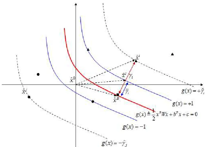
Figure 3.1: The Separating Quadratic Curve

(b, c) ∈ _Rm+1_{, the related gradient direction at point} _x_ˆi _{with respect to the quadratic}

surface g(x) =g(ˆxi) intercepts the quadratic surface g(x) = 0 at a point xˆB. The length of the segment ˆxi_x_ˆB_{, denoted as} _γ

i, is called the geometrical margin at point ˆxi with

respect to the quadratic surface g(x) = 0.

quadratic functiong(x) = 1₂xT_W_x+bT_x+c_{, where}_W ₌_WT _∈

Rm×m and(b, c)∈Rm+1,

the related gradient direction at pointˆxi _{with respect to the quadratic surface}_{g(x) =} _g(ˆ_xi₎

intercepts the surface g(x) = +1 (or −1) at a point ˆxi. The length of the segment ˆxi_ˆ_xB_,

denoted as γ¯i, is called the relative geometrical margin at the point xˆi with respect to the

quadratic surface g(x) = 0.

Figure 3.1 illustrates the ˆxi_,_ˆ_xi_,_x_ˆB_{, ˆ}_γ

i,γi and ¯γi form= 2, where g(x) = 0 is the red

separating quadratic curve. Expression (4) can deduct that ˆγi = ˆyig(ˆxi)≥1, i= 1,· · · , n,

which indicates that each training point has a no-less-than one functional margin. Moreover, the relative geometrical margin ¯γi at the pointˆxi can be approximated as

(35)

ThusˆxB ₌_ˆ_xi₋_γ_¯ i

∇g(ˆxi₎ k∇g(ˆxi₎_k

2. Taylor’s expansion says thatg(ˆx

B₎_≈_g(ˆ_xi₎₊_∇_g(ˆ_xi₎T_(ˆ_xB₋_ˆ_xi_).

Noting that g(ˆxB) = 0 and g(ˆxi) = 1, we have ¯γi ≈ k∇g(ˆx

i₎_k

2

∇g(ˆxi₎T_∇_g₍_ˆ_xi₎. Similarly, g(ˆxi)≈g(ˆxi) +∇g(ˆxi)T(ˆxi−ˆxi)

g(ˆxi)≈g(ˆxi) +∇g(ˆxi)T(ˆxi−ˆxi)

andxˆi−ˆxi =− γi−γ¯i k∇g(ˆxi₎_k

2∇g(ˆx

i_{), which is inferred by}−−→_ˆ_x0_ˆ_xi₋−−→_ˆ_x0_ˆ_xi ₌−−→_ˆ_xi_ˆ_xi_{. Hence}_∇_g(ˆ_xi₎T_∇_g

(ˆxi₎ _{≈ ∇}_g(ˆ_xi₎T_∇_g_(ˆ_xi_{). Consequently, at point} _x_ˆi_{, ¯}_γ

i = kˆxB −xˆik2 ≈

k∇g(ˆxi)k2

∇g(ˆxi₎T_∇_g₍_ˆ_xi₎ ≈

1

k∇g(ˆxi₎_k

2 =

1

kWxˆi₊_b_k

2. Note that, in general, ¯γi 6= ¯γj for ˆx

i ₆₌_ˆ_xj_{. This situation is different}

from that in the SVM model.

The objective of the QSSVM model can be stated as “to maximize the sum of the rela-tive geometrical margins at all training points with respect to a quadratic surfaceg(x) = 0 subject to the condition that each training point has a no-less-than one functional mar-gin”(See Figure 3.1, where the distance between the two blue curves is maximized subject to the condition that no training point exists between the two blue curves.).

For a quadratically separable training data set {(ˆx1_,_y_ˆ1_),_{· · ·} _,_(ˆ_xn_,_y_ˆn₎_}_{, we first}

max-imize the relative geometrical margin of a training point xˆi _{with respect to a quadratic}

surface g(x) = 0 subject to the condition that each training point has a no-less-than one functional margin, which can be formulated as

max 1

kWxˆi₊_b_k

2

s.t. yˆi(1 2(ˆx

i₎T_W_x_ˆi₊_bT_ˆ_xi₊_c)_≥_{1, i}_{= 1,}_{· · ·} _{, n,}

W =WT ∈_Rm×m_, _{(b, c)}_∈

Rm+1,

excluding the trivial case of kWˆxi₊_b_k

2 = 0. This problem is equivalent to

min kWˆxi+bk2 2

s.t. yˆi(1 2(ˆx

i₎T_W_ˆ_xi₊_bT_ˆ_xi₊_c)_≥_{1, i}_{= 1,}_{· · ·}_{, n,}

W =WT ∈_Rm×m_, _{(b, c)}_∈

(36)

Forn training points, we may consider the following aggregated model:

min

n

X

i=1

kWˆxi+bk2 2

s.t. yˆi(1 2(ˆx

i₎T_W_ˆ_xi₊_bT_ˆ_xi₊_c)_≥_{1, i}_{= 1,}_{· · ·}_{, n,} _(QSSVM)

W =WT ∈_Rm×m_, _{(b, c)}_∈

Rm+1.

However, if the training data set is not quadratically separable, for a separating quadratic surfaceg(x) = 0, one of the following two situations would occur for some training points:

Situation 1 : for point ˆxi,yˆi =−1, but 1 2(ˆx

i₎T_W_ˆ_xi₊_bT_ˆ_xi₊_{c >} ₋_1,

Situation 2 : for point ˆxj,yˆj = +1, but 1 2(ˆx

j₎T_W_ˆ_xj₊_bT_ˆ_xj ₊_{c <}_1.

These points are referred to as the outliers of the data set with respect to the quadratic surface g(x) = 0. In this case, the proposed model (QSSVM) would become infeasible, since no quadratic surface can separate all training points into their corresponding classes correctly. To take care of this situation, similar to the development of the soft SVM model, we add a slack variableξi ≥0 for each constraint in the model (QSSVM) and a number

ˆ

η > 0 as the penalty value for each ξi in the objective function. Then we consider the

following soft QSSVM model:

min

n

X

i=1

kWxˆi+bk2 2+ ˆη

n

X

i=1

ξi

s.t. yˆi(1 2(ˆx

i

)TWxˆi+bTˆxi +c)≥1−ξi, i= 1,· · · , n, (SQSSVM)

W =WT ∈_Rm×m, (b, c)∈_Rm+1, ξi ≥0, i= 1,· · · , n.

Notice that in models (QSSVM) and (SQSSVM), the matrixW is symmetric. To simplify these two models, we may convert each of them into an equivalent form as follows. First, let ¯W be the vector formed by taking the m2₂+m elements of the upper triangle part of the matrix W, i.e.,

¯

W =hw11 w12 · · · w1m w22 w23 · · · w2m · · · wmm

iT

(37)

Then, construct anm×(m2+m

2 ) matrixM

i_{for the training point}_x_ˆi _{= [ˆ}_xi

1,xˆi2,· · ·,xˆim]T ∈

Rm as follows. For thej-th row of Mi in R

m2+m

2 , j = 1,· · · , m, check the elements of ¯W

one by one. If the p-th element of ¯W is wjk or wkj for some k= 1,2,· · · , m, then assign

the p-th element of thej-th row of Mi _{to be ˆ}_xi

k. Otherwise, assign it to be 0.

Takem = 3 as an example:

W =   

w11 w12 w13

w12 w22 w23

w13 w23 w33

 

⇒ W¯ = h

w11 w12 w13 w22 w23 w33

iT

⇒Mi =    ˆ

xi₁ xî₂ xî₃ 0 0 0 0 xî₁ 0 xî₂ xî₃ 0 0 0 xî₁ 0 xî₂ xî₃

  

Also let matrixHi = h

Mi_{, I}i_∈

Rm×(

m2+m

2 +m), i= 1,· · · , n, whereI is them-dimensional

identity matrix. Then, define the vector of variables z= "

¯ W

b #

∈_Rm2+32 m and the vector

ˆsi =[1 2xˆ

i

1xˆ

i

1,· · · ,xˆ

i

1xˆ

i m,

1 2xˆ

i

2xˆ

i

2,· · · ,xˆ

i

2xˆ

i m,· · · ,

1 2xˆ

i m−1xˆ

i m−1,xˆ

i m−1xˆ

i m,

1 2xˆ

i mxˆ

i m,

ˆ

xi₁, ,xˆi₂,· · · ,xˆi_m]∈_R(m+1)2 m+m.

The objective of model (QSSVM) becomes

Pn

i=1kWˆx

i₊_b_k2 2 =

Pn

i=1kH

i_z_k2 2 =

Pn

i=1(H

i_z)T_(Hi_z)

=Pn

i=1zT(Hi)THiz=zT(

Pn

i=1(Hi)THi)z.

Let G=Pn

i=1(Hi)THi ∈R

(m2+3₂ m)×(m2+3₂ m)_{, then the model (QSSVM) becomes}

min zTGz

(38)

Similarly, the model (SQSSVM) can be reformulated as

min zTGz+ ˆη

n

X

i=1

ξi

s.t. yˆi((ˆsi)Tz+c)≥1−ξi, i= 1,· · · , n, (SQSSVM0)

(z, c)∈_Rm2+32 m+1, ξ_i ≥0, i= 1,· · · , n.

This kernel-free soft QSSVM model is proposed for binary classification directly using a quadratic function to separate the data set. Notice that G is positive semidefinite since zT_Gz₌_zT Pn

i=1(H

i₎T_Hi_z₌ Pn

i=1kH

i_z_k2

2 ≥ 0 for any z∈ R

m2+3m

2 . Consequently,

both of models (QSSVM0) and (SQSSVM0) are convex linearly constrained quadratic programming (LCQP) problems [36].

3.3 Some Properties of the Soft QSSVM Model

In this section, we study some properties of the model (SQSSVM0). For any given training data set {(ˆx1_,_y_ˆ1_),_{· · ·} _,_(ˆ_xi_,_y_ˆi_),_{· · ·} _,_(ˆ_xn_,_y_ˆn₎_} _{and ˆ}_{η >} _{0, the solvability of the model}

(SQSSVM0) is studied in the next result.

Theorem 3.3.1. For any given training data set{(ˆx1_,_y_ˆ1_),_{· · ·} _,_(ˆ_xi_,_y_ˆi_),_{· · ·} _,_(ˆ_xn_,_y_ˆn₎_}_and

ˆ

η > 0, there exists an optimal solution to the model (SQSSVM0) with a finite objective value.

Proof. Take arbitrary (˜z,˜c)∈_Rm2+32m+2 and let

˜

ξi = max{0,1−yˆi((ˆsi)T˜z+ ˜c)}, i= 1,· · · , n.

It is easy to see that (˜z,˜c,ξ) is feasible to the model (SQSSVM˜ 0). Notice that the objective function is continuous and the feasible domain is a closed convex set defined by linear inequalities. Moreover, for any z∈_Rm2+32 m and ξ_i ≥0, i= 1,· · · , n,zTGz+ ˆηPn

i=1ξi =

Pn

i=1(kHizk22+ ˆηξi) ≥ 0, which indicates that the objective value is bounded below by

0 over the feasible domain. Hence there must exist an optimal solution with a finite objective value.

(39)

the next result states the relationship between the optimal solutions of models (QSSVM0) and (SQSSVM0).

Theorem 3.3.2. For any given η >ˆ 0, let (zˆη_{, c}ˆη_,_ξηˆ₎ _{be an optimal solution of model}

(SQSSVM0) and assume that the sequence {(zηˆ_{, c}ηˆ_,_ξηˆ₎_} _{converges to} _(z∗_{, c}∗_,_ξ∗₎ _as _η_ˆ_→

∞. If the training data set is quadratically separable, thenξ∗ =0(where0= (0,· · · ,0)T _∈

Rn) and (z∗, c∗) is an optimal solution of model (QSSVM0).

Proof. When the training data set is quadratically separable, it is not difficult to see that there exists a feasible solution (ˆz,ˆc,0) to the model (SQSSVM0) with a given ˆη >0. We first prove that Pn

i=1ξ ˆ

η

i → 0 as ˆη → ∞ by contradiction. Suppose that there exists a

givenδ >0 such that for any ˆη ≥ηˆ∗ _, ˆzTG_δˆz+1 >0, we have|Pn

i=1ξ ˆ

η

i −0|=

Pn

i=1ξ ˆ

η i ≥δ.

Then, for the optimal solution (zηˆ_{, c}ηˆ_,_ξηˆ_{) of model (SQSSVM}0_{) with any given ˆ}_η _≥ _η_ˆ∗_, we have

zη Tˆ Gzηˆ+ ˆη

n

X

i=1

ξ_iηˆ ≥0 + ˆη∗δ= 0 +ˆzTGˆz+ 1>ˆzTGˆz+ 0

sinceGis positive semidefinite. Therefore, for any given ˆη ≥ηˆ∗, (zηˆ_{, c}ηˆ_,_ξηˆ_{) can not be an}

optimal solution because (ˆz,c,ˆ 0) is feasible to the model (SQSSVM0). This contradiction leads to that Pn

i=1ξ ˆ

η

i →0 as ˆη→ ∞. Consequently, ξηˆ →ξ

∗ ₌₀ _{as ˆ}_η _{→ ∞}_.

Next, we prove that (z∗, c∗) is an optimal solution to model (QSSVM0). Since (zηˆ_{, c}ηˆ_,_ξηˆ₎

is feasible to the model (SQSSVM0) for all ˆη >0 and the linear constraints are in a closed form, we have {(zηˆ, cηˆ,ξηˆ)} converges to (z∗, c∗,0) as ˆη→ ∞, and

ˆ

yi((ˆsi)Tz∗+c∗)≥1, i= 1,· · · , n.

Hence (z∗, c∗) is feasible to model (QSSVM0). Moreover, let (¯z,¯c) be an optimal solution to model (QSSVM0). Then (¯z,¯c,0) is feasible to model (SQSSVM0). Consequently, we have

zη Tˆ Gzηˆ+ ˆη

n

X

i=1

ξ_iηˆ ≤¯zTG¯z+ 0.

Let ˆη → ∞and assume that 0∗ ∞= 0 without loss of generality, then we havez∗TGz∗ ≤

(40)

Let F∗ ₌ _{_{(z, c,}_ξ) _∈

R

m2+3m

2 ×_R1×_Rn|(z, c,ξ) is an optimal solution to the model

(SQSSVM0)}. Then F∗ ₆₌_∅ _{by Theorem 3.3.1. Moreover, we have the next three results.} Theorem 3.3.3. For any given training data set{(ˆx1_,_y_ˆ1_),_{· · ·} _,_(ˆ_xi_,_y_ˆi_),_{· · ·} _,_(ˆ_xn_,_y_ˆn₎_}_and

ˆ

η >0, if G is positive definite, then the optimal solution of model (SQSSVM0) is unique with respect to the variable z.

Proof. Assume that (ˆz,ˆc,ξ)ˆ ∈ F∗_{, (¯}_z,_c,_¯ _ξ)_¯ _{∈ F}∗ _and _ˆ_z ₆₌ _¯_{z. For any 0} _{< δ <} _1, (˜z,˜c,ξ)˜ _,δ(ˆz,ˆc,ξ) + (1ˆ −δ)(¯z,¯c,ξ) is feasible to model (SQSSVM¯ 0) due to the convexity of the feasible domain. Therefore,

˜zTG˜z+ ˆη

n

X

i=1

˜

ξi ≥ˆzTGˆz+ ˆη n

X

i=1

ˆ ξi,

˜zTG˜z+ ˆη

n

X

i=1

˜

ξi ≥¯zTG¯z+ ˆη n

X

i=1

¯ ξi.

Multiplying the first inequality by δ and the second by (1−δ), we have

˜

zTG˜z+ ˆη

n

X

i=1

˜

ξi ≥δˆzTGˆz+ (1−δ)¯zTG¯z+ ˆη n

X

i=1

(δξˆi+ (1−δ) ¯ξi).

Equivalently, [δˆz+ (1−δ)¯z]TG[δˆz+ (1−δ)¯z]≥δˆzTGˆz+ (1−δ)¯zTG¯z, and δ(1−δ)(ˆz−

¯z)TG(ˆz−¯z) ≤ 0. When G is positive definite, we have ˆz−¯z = 0, which contradicts to the assumption that ˆz6=¯z.

Thus, for any given training data set, ifGis positive definite, the main characteristics of the separating quadratic surface are uniquely determined by the optimal solution of model (SQSSVM0) with respect to the variable z.

Theorem 3.3.4. For any given training data set{(ˆx1_,_y_ˆ1_),_{· · ·} _,_(ˆ_xi_,_y_ˆi_),_{· · ·} _,_(ˆ_xn_,_y_ˆn₎_}_and

ˆ

η >0, ifG is positive definite, then there exist constants c andc such that c≤c≤c, for any (z, c,ξ)∈ F∗_.

Proof. Let (ˆz,ˆc,ξ)ˆ ∈ F∗_{. When} _G _{is positive definite, by Theorem 3.3.3,} _ˆ_z _{is uniquely} determined and, for each (z, c,ξ)∈ F∗_{, we have} _z₌_ˆ_z _and _zT_Gz_{+ ˆ}_ηPn

i=1ξi =ˆzTGˆz+

ˆ ηPn

i=1ξˆi. Consequently,

Pn

i=1ξi =

Pn

(41)

ξi ≥0 for anyi, we have ξi ≤Pn_i₌₁ξi = ¯δ. Therefore,

c≤ξj−1−(ˆsj)Tˆz≤δ¯−1−(ˆsj)Tˆz, for j ∈ {j : ˆyj =−1}

c≥1−ξj−(ˆsj)Tˆz≥1−δ¯−(ˆsj)Tˆz, for j ∈ {j : ˆyj = +1}.

Let c = min{j:ˆyj₌₋₁_}{δ¯−1−(ˆsj)Tˆz}, c = max_{_j_:ˆ_yj₌₊₁_}{1−δ¯−(ˆsj)Tˆz}, then we have c≤c≤c.

Theorem 3.3.5. If the training data set is quadratically separable and Gis positive defi-nite, then for any given sufficiently largeη >ˆ 0, the optimal solution of model(SQSSVM0)

is unique with respect to the variable c.

Proof. When the training data set is quadratically separable, by a similar proof of Theorem 3.3.2, for the model (SQSSVM0) with any given sufficiently large ˆη > 0 and (˘z,˘c,ξ)˘ ∈ F∗_{, we know} _ξ_˘₌_{0. Hence (˘}_z,_c,_˘ _{0) is feasible to the model (SQSSVM}0_{), which} indicates that ˆyi₍₍_ˆ_si₎T_˘_z_{+ ˘}_c)_≥_1,_∀_{i. We first prove that there exists a}_j _{∈ {}_j _{: ˆ}_yj _{= +1}_}

such that ˆyj_((ˆ_sj₎T_˘_z_{+ ˘}_{c) = 1 as follows by contradiction.}

Assume this conclusion is wrong, then we have

(ˆsj)T˘z+ ˘c >1, for j ∈ {j : ˆyj = +1}, (B1) (ˆsj)T˘z+ ˘c≤ −1, forj ∈ {j : ˆyj =−1}. (B2)

Let˜z=δ˘z and ˜c=δ(˘c+ 1)−1, for some δ ∈(0,1). Then expression (B2) is equivalent to

(ˆsj)T˜z+ ˜c≤ −1, for j ∈ {j : ˆyj =−1} (B3)

Moreover, for j ∈ {j : ˆyj =−1}, from expression (B1), we have

lim

δ→1−[(ˆs

j₎T_˜_z_{+ ˜}_{c] = lim} δ→1−[δ(ˆs

j₎T_˘_z₊_δ(˘_c_{+ 1)}₋_{1] = (ˆ}_sj₎T_˘_z_{+ ˘}_{c >} _1.

Hence there exists a δ ∈(0,1) such that

(ˆsj)T˜z+ ˜c >1, forj ∈ {j : ˆyj = +1}. (B4)

(42)

the corresponding objective value is ˜zT_G˜_z_{+ 0 =} _δ2_z_˘T_G˘_z _<_˘_zT_G˘_z_{+ 0, which indicates}

that (˘z,c,˘ 0) is not an optimal solution. This contradiction infers that there exists a j ∈ {j : ˆyj _{= +1}_} _{such that ˆ}_yj_((ˆ_sj₎T_˘_z_{+ ˘}_{c) = 1.}

Suppose that the model (SQSSVM0) has another optimal solution (ˆz,ˆc,ξ). As before,ˆ we have ˆξ =0. WhenG is positive definite, we know˘z=ˆzfrom Theorem 3.3.3. Rewrite the two optimal solutions as (˘z,˘c,0) and (˘z,ˆc,0), respectively. From the above arguments, we know there exist j and ¯j ∈ {j : ˆyj = +1}such that

(ˆs¯j)T˘z+ ˘c= 1, (ˆsj)T˘z+ ˘c≥1, (ˆsj)T˘z+ ˆc= 1, (ˆs¯j)T˘z+ ˆc≥1.

Therefore, we have ˘c≥ˆcand ˘c≤cˆusing the above expressions. In other words, we have ˘

c= ˆc.

From Theorems 3.3.3 and 3.3.5, we know that if the training data set is quadratically separable and G is positive definite, then, for any sufficiently large ˆη > 0, the model (SQSSVM0) generates a unique separating quadratic surface. Generally speaking, for any given training data set with G being positive definite, we may solve the model (SQSSVM0) with a sufficiently large ˆη >0 to generate a separating quadratic surface for binary classification.

Notice that if the matrix G in model (SQSSVM0) is only positive semidefinite, we can always append a perturbation such that the matrix G+I ( >0, I is the identity matrix) becomes positive definite. Then, consider the following perturbed model:

min zT(G+I)z+ ˆη

n

X

i=1

ξi

s.t. yˆi((ˆsi)Tz+c)≥1−ξi, i= 1,2,· · · , n. (SQSSVM0-)

(z, c)∈_Rm2+32m+2, ξ

i ≥0, i= 1,· · · , n.

(43)

Lemma 3.3.1. For any given training data set {(ˆx1_,_y_ˆ1_),_{· · ·}_,_(ˆ_xi_,_y_ˆi_),_{· · ·} _,_(ˆ_xn_,_y_ˆn₎_} _and

ˆ

η > 0, if the optimal value of model (SQSSVM0) is v and the optimal value of model

(SQSSVM0-) is v, for a given >0, then v →v as →0.

Proof. Let (˜z,c,˜ ξ)˜ ∈ F∗_{. If}_k_z_˜_{k 6}_{= 0, for (z}_{, c}_,_ξ_{) and any}_{δ >}_{0, there exists}

0 = ₍_˜_zTδ₎₍_˜_z₎ such that when 0< < 0,

v ≤zTGz+ ˆη

n

X

i=1

ξ_i ≤v≤˜zT(G+I)˜z+ ˆη n

X

i=1

˜

ξi =v+(˜z)T(˜z)< v+δ.

That is,|v−v|< δ. If k˜zk= 0, by the expression

v ≤zTGz+ ˆη

n

X

i=1

ξ_i ≤v ≤˜zT(G+I)˜z+ ˆη n

X

i=1

˜

ξi =v+(˜z)T(˜z) =v.

we have thatv =v. Therefore, v →v as→0.

Remark 1. For any given η >ˆ 0 and 0< 1 < 2, we have

v1 ≤(z

2₎T_Gz2 ₊

1(z2)T(z2) + ˆη

n

X

i=1

ξ2

i

<(z2₎T_Gz2 ₊

2(z2)T(z2) + ˆη

n

X

i=1

ξ2

i =v2.

Hence the sequence {v} monotonically decreases to v as &0.

Theorem 3.3.6. For any given training data set{(ˆx1,yˆ1),· · · ,(ˆxi,yˆi),· · · ,(ˆxn,yˆn)}and

ˆ

η >0, if the sequence{(z_{, c}_,_ξ₎_}_{converges to}_(z0_{, c}0_,_ξ0₎_as_→₀_{, then}_(z0_{, c}0_,_ξ0₎_{∈ F}∗

and z0T_z0 _≤_zT_z_{, for any} _{(z, c,}_ξ)_{∈ F}∗_.

Proof. When {(z_{, c}_,_ξ₎_{} →} _(z0_{, c}0_,_ξ0_{) as} _→ _{0, obviously (z}0_{, c}0_,_ξ0_{) is feasible to}

model (SQSSVM0). By Lemma 3.3.1, we have v → v as → 0. Hence we know

(z0_{, c}0_,_ξ0₎_{∈ F}∗_.

Quadratic Surface Support Vector Machines with Applications.

ABSTRACT

DEDICATION

BIOGRAPHY

ACKNOWLEDGEMENTS

TABLE OF CONTENTS

LIST OF TABLES

LIST OF FIGURES

Chapter 1

INTRODUCTION

1.1

Historic Background of Support Vector Machines

1.2

Statement of Problems

1.3

Motivations

1.4

Outline

Chapter 2

LITERATURE REVIEW

2.1

Data Classification Methods

2.2

Support Vector Machine Models

2.3

Fuzzy Support Vector Machine Models

2.4

Fisher Discriminant Analysis

2.5

Linearly Constrained Quadratic Programming

Problems

2.6

Decomposition Programming

Chapter 3

SOFT QSSVM MODEL

3.1

Introduction

3.2

Quadratic Surface Support Vector Machine

Mod-els

3.3

Some Properties of the Soft QSSVM Model