ABSTRACT
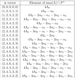
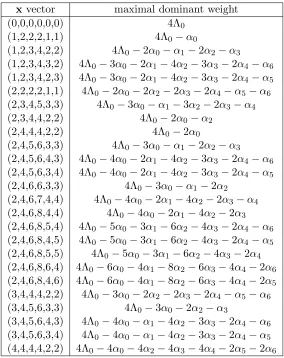
CRIFO, SUZANNE ELISE. Some Maximal Dominant Weights and Their Multiplicities for Affine Lie Algebra Representations. (Under the direction of Kailash Misra).
It is known that there are finitely many maximal dominant weights for an integrable highest weight module of an affine Lie algebra g. However, a description for these maximal dominant weights is known in only select cases. For example, Jayne and Misra studied the maximal dominant weights of theA(1)n -modulesV((k−1)Λ0+ Λs) where 0≤s≤n. In this thesis we give
Some Maximal Dominant Weights and Their Multiplicities for Affine Lie Algebra Representations
by
Suzanne Elise Crifo
A dissertation submitted to the Graduate Faculty of North Carolina State University
in partial fulfillment of the requirements for the Degree of
Doctor of Philosophy
Mathematics
Raleigh, North Carolina 2019
APPROVED BY:
Negash Medhin Radmila Sazdanovic
DEDICATION
BIOGRAPHY
ACKNOWLEDGEMENTS
The author would like to thank her advisor, Kailash Misra, for his continuous support and guidance throughout the years, without which this thesis would not have been possible. The author also thanks the rest of her committee members, Ernest Stitzinger, Radmila Sazdanovic, and Negash Medhin, for their advice and input. Additionally, the author would like to thank the following individuals from North Carolina State University for their support and mentorship: Molly Fenn, John Griggs, Vanessa Doriott Anderson, and Di Bucklad.
The author would like to thank her undergraduate professor David Damiano, who encour-aged her to pursue a graduate education in mathematics and continued to provide mentorship beyond her time at Holy Cross.
TABLE OF CONTENTS
LIST OF TABLES . . . vi
LIST OF FIGURES . . . ix
Chapter 1 Introduction . . . 1
Chapter 2 Kac-Moody Algebras and their Representations . . . 3
2.1 Lie Algebras . . . 3
2.1.1 Representations and Modules . . . 5
2.2 Kac-Moody Algebras . . . 6
2.2.1 Integrable Highest Weight Modules . . . 10
Chapter 3 Maximal Dominant Weights of V(kΛ0) . . . 13
3.1 Introduction . . . 13
3.2 TypeA(1)n . . . 14
3.3 TypeBn(1) . . . 15
3.4 TypeCn(1) . . . 28
3.5 TypeD(1)n . . . 35
3.6 TypeG(1)2 . . . 44
3.7 TypeF4(1) . . . 48
3.8 TypeE(1)6 . . . 52
3.9 TypeE(1)7 . . . 58
3.10 TypeE(1)8 . . . 66
3.11 TypeA(2)2n . . . 73
3.12 TypeA(2)2n−1 . . . 78
3.13 TypeD(2)n+1 . . . 86
3.14 TypeE(2)6 . . . 93
3.15 TypeD(3)4 . . . 96
Chapter 4 Crystal Bases . . . .100
4.1 Introduction . . . 100
4.2 Crystal Bases . . . 102
4.3 Perfect Crystals . . . 105
4.4 Path Realizations . . . 106
Chapter 5 Weight Multiplicities. . . .111
5.1 Introduction . . . 111
5.2 TypeA(1)n . . . 112
5.3 TypeBn(1) . . . 112
5.4 TypeCn(1) . . . 117
5.5 TypeD(1)n . . . 122
LIST OF TABLES
Table 3.1 A(1)2 , max(kΛ0)∩P+. . . 16
Table 3.2 A(1)3 , max(kΛ0)∩P+. . . 16
Table 3.3 A(1)4 , max(kΛ0)∩P+. . . 17
Table 3.4 B5(1), max(2Λ0)∩P+. . . 21
Table 3.5 B6(1), max(2Λ0)∩P+. . . 22
Table 3.6 B5(1), max(3Λ0)∩P+. . . 27
Table 3.7 B6(1), max(3Λ0)∩P+. . . 28
Table 3.8 B5(1), max(4Λ0)∩P+. . . 29
Table 3.9 B6(1), max(4Λ0)∩P+. . . 30
Table 3.10 C5(1), max(2Λ0)∩P+. . . 34
Table 3.11 C6(1), max(2Λ0)∩P+. . . 35
Table 3.12 C5(1), max(3Λ0)∩P+. . . 36
Table 3.13 C6(1), max(3Λ0)∩P+. . . 37
Table 3.14 D(1)5 , max(2Λ0)∩P+ . . . 41
Table 3.15 D(1)6 , max(2Λ0)∩P+ . . . 42
Table 3.16 D(1)5 , max(3Λ0)∩P+ . . . 43
Table 3.17 D(1)6 , max(3Λ0)∩P+ . . . 43
Table 3.18 D(1)5 , max(4Λ0)∩P+ . . . 44
Table 3.19 D(1)6 , max(4Λ0)∩P+ . . . 45
Table 3.20 G(1)2 , max(2Λ0)∩P+. . . 47
Table 3.21 G(1)2 , max(3Λ0)∩P+. . . 47
Table 3.22 G(1)2 , max(4Λ0)∩P+. . . 47
Table 3.23 G(1)2 , max(6Λ0)∩P+. . . 48
Table 3.24 F4(1), max(2Λ0)∩P+. . . 51
Table 3.25 F4(1), max(3Λ0)∩P+. . . 51
Table 3.26 F4(1), max(4Λ0)∩P+. . . 52
Table 3.27 E6(1), max(2Λ0)∩P+. . . 57
Table 3.28 E6(1), max(3Λ0)∩P+. . . 57
Table 3.29 E6(1), max(4Λ0)∩P+. . . 58
Table 3.30 E7(1), max(2Λ0)∩P+. . . 64
Table 3.31 E7(1), max(3Λ0)∩P+. . . 65
Table 3.32 E7(1), max(4Λ0)∩P+. . . 65
Table 3.33 E8(1), max(2Λ0)∩P+. . . 71
Table 3.34 E8(1), max(3Λ0)∩P+. . . 72
Table 3.35 E8(1), max(4Λ0)∩P+. . . 72
Table 3.36 A(2)10, max(2Λ0)∩P+ . . . 76
Table 3.37 A(2)12, max(2Λ0)∩P+ . . . 76
Table 3.38 A(2)10, max(3Λ0)∩P+ . . . 77
Table 3.40 A(2)10, max(4Λ0)∩P+ . . . 78
Table 3.41 A(2)12, max(4Λ0)∩P+ . . . 79
Table 3.42 A(2)9 , max(2Λ0)∩P+ . . . 82
Table 3.43 A(2)11, max(2Λ0)∩P+ . . . 83
Table 3.44 A(2)9 , max(3Λ0)∩P+ . . . 84
Table 3.45 A(2)11, max(3Λ0)∩P+ . . . 84
Table 3.46 A(2)9 , max(4Λ0)∩P+ . . . 85
Table 3.47 A(2)11, max(4Λ0)∩P+ . . . 85
Table 3.48 D(2)6 , max(2Λ0)∩P+ . . . 89
Table 3.49 D(2)7 , max(2Λ0)∩P+ . . . 89
Table 3.50 D(2)6 , max(3Λ0)∩P+ . . . 90
Table 3.51 D(2)7 , max(3Λ0)∩P+ . . . 90
Table 3.52 D(2)6 , max(4Λ0)∩P+ . . . 91
Table 3.53 D(2)7 , max(4Λ0)∩P+ . . . 92
Table 3.54 E6(2), max(2Λ0)∩P+. . . 95
Table 3.55 E6(2), max(3Λ0)∩P+. . . 95
Table 3.56 E6(2), max(4Λ0)∩P+. . . 96
Table 3.57 D(3)4 , max(2Λ0)∩P+ . . . 98
Table 3.58 D(3)4 , max(3Λ0)∩P+ . . . 98
Table 3.59 D(3)4 , max(4Λ0)∩P+ . . . 98
Table 3.60 D(3)4 , max(6Λ0)∩P+ . . . 99
Table 5.1 B3(1), multiplicities of max(2Λ0)∩P+ . . . 114
Table 5.2 B4(1), multiplicities of max(2Λ0)∩P+ . . . 115
Table 5.3 B3(1), multiplicities of max(3Λ0)∩P+ . . . 116
Table 5.4 C2(1), multiplicities of max(2Λ0)∩P+ . . . 119
Table 5.5 C2(1), multiplicities of max(3Λ0)∩P+ . . . 119
Table 5.6 C2(1), multiplicities of max(4Λ0)∩P+ . . . 120
Table 5.7 C2(1), multiplicities of max(5Λ0)∩P+ . . . 121
Table 5.8 C3(1), multiplicities of max(2Λ0)∩P+ . . . 122
Table 5.9 C3(1), multiplicities of max(3Λ0)∩P+ . . . 123
Table 5.10 C4(1), multiplicities of max(2Λ0)∩P+ . . . 124
Table 5.11 C4(1), multiplicities of max(3Λ0)∩P+ . . . 124
Table 5.12 C4(1), multiplicities of max(4Λ0)∩P+ . . . 125
Table 5.13 D(1)4 , multiplicities of max(2Λ0)∩P+ . . . 128
Table 5.14 D(1)4 , multiplicities of max(3Λ0)∩P+ . . . 129
Table 5.15 D(1)5 , multiplicities of max(2Λ0)∩P+ . . . 130
Table 5.16 D(1)5 , multiplicities of max(3Λ0)∩P+ . . . 131
Table 5.17 D(1)6 , multiplicities of max(2Λ0)∩P+ . . . 132
LIST OF FIGURES
Chapter 1
Introduction
Sophus Lie discovered Lie algebras in the 19th century while studying the symmetries of solu-tions of differential equasolu-tions. Since then, Lie algebras have been studied extensively and have been shown to have many connections to other areas in mathematics and mathematical physics. By the end of the 19th century, Wilhelm Killing and ´Elie Cartan had classified all simple finite-dimensional complex Lie algebras [4]. Independently and simultaneously, Victor Kac [10] and Robert Moody [21] discovered Kac-Moody algebras. Kac-Moody algebras are a generalization of finite dimensional complex semisimple Lie algebras. Kac-Moody algebras are divided into three subcategories: finite dimensional semisimple Lie algebras, infinite dimensional affine Lie algebras of polynomial growth, and infinite dimensional algebras of exponential growth. This thesis is concerned with the second subcategory, which are called affine Lie algebras.
In 1974, Kac [11] introduced the notion of an integrable highest-weight representation, al-lowing the representation theory of finite dimensional semisimple Lie algebras to expand from the finite dimensional case to affine Lie algebras. To describe the structure of an integrable highest-weight representation, one needs to describe its maximal dominant weights. The max-imal weights form a type of “ceiling” to the set of all weights. Any other weight lies on an infinite string off a maximal weight. Any maximal weight is Weyl group conjugate to a maxi-mal dominant weight.
It is known there are finitely many maximal dominant weights for any integrable highest weight representation of an affine Lie algebra. However, determining these maximal dominant weights is a nontrivial task. Tsuchioka found all maximal dominant weights for modules of the formV(Λ0+Λs) where 0≤s < pfor typeA(1)p−1[23]. This work was generalized in 2014 by Jayne and Misra, who found all maximal dominant weights for modules of the formV((k−1)Λ0+ Λs)
where 0 ≤ s ≤ n−1 for type A(1)n−1 [7]. In 2017, Kim, Lee, and Oh determined all maximal dominant weights for V(Λ) where Λ is of level 2 for types Bn(1), D(1)n , A(2)2n−1, A
(2) 2n, D
(2)
n+1,and of level 1 forCn(1) [18].
multiplicities can be studied using a combinatorial tool that comes out of studying quantum groups. Quantum groups (which are not actually groups), were introduced independently by Drinfel0d [2] and Jimbo [9] in 1985. The quantum group is a q-deformation of the univer-sal enveloping algebra of a symmetrizable Kac-Moody algebra. Lusztig [19] proved that the representation theory of this quantum group is the same as the representation theory of the corresponding Kac-Moody algebra. This means that the weight spaces (and their dimensions) are invariant under this deformation.
The representation theory of quantum groups is more easily studied than that of Kac-Moody algebras due to those combinatorial tools we hinted at earlier. The notion of acrystal basis was introduced by Kashiwara [17] in 1990 and is the same as Lusztig’s [20] canonical base at q= 0. Crystals allow us to study these multiplicities. Specifically, we useperfect crystals, whose theory is given in [15] and [14]. These perfect crystals give rise to a path realization [15], [14] of crystals for integrable highest weight modules of affine Lie algebras. This path model obtains a colored, oriented graph, called thecrystal graph, for irreducible highest weight modules over affine Lie algebras, allowing us to find the multiplicities of maximal dominant weights by counting the number of vertices corresponding to each weight.
This dissertation expands on the results listed above by finding maximal dominant weights for the remaining affine Lie algebras in the case of V(kΛ0) and some of the multiplicities of these weights. Chapter 2 gives the background necessary to find the maximal dominant weights, which are found in Chapter 3. We also include the relevant results from [7] for type A(1)n and
prove our findings are the same as [18] in the casek= 2 for the appropriate affine Lie algebras in Chapter 3. Chapter 4 then gives the information needed to study path realizations of integrable highest weight modules. In Chapter 5, we include the results from [15] that are used to study the path realizations of V(kΛ0) in types Bn(1), Cn(1), and D(1)n , as well as the relevant results
Chapter 2
Kac-Moody Algebras and their
Representations
In this chapter, we discuss Kac-Moody algebras and their representations. As noted below, Kac-Moody algebras fall into three classes. Of the three classes, we will focus on affine Lie algebras and their representations. Unless otherwise noted, we will assume the field is C.
2.1
Lie Algebras
Definition 2.1.1. A Lie algebra overCis a vector space L equipped with a product, called a
Lie bracket, [·,·] :L×L→Lthat satisfies the following properties:
• Bilinearity: [ax+by, z] =a[x, z] +b[y, z] and [x, ay+bz] =a[x, y] +b[x, z], • Alternativity: [x, x] = 0,
• Jacobi Identity: [x,[y, z]] = [[x, y], z] + [y,[x, z]], for all x, y, z∈Land a, b∈C.
Note that because the Lie bracket is both bilinear and alternative, one can show that it is also skew-symmetric, or [x, y] =−[y, x] for all x, y∈L.
While there are many examples of finite dimensional Lie algebras, a familiar one isR3 with
the cross product of vectors serving as the Lie bracket.
Example2.1.2. For any vector spaceV, the set of linear operators onV is a Lie algebra, denoted
gl(V) with the Lie bracket defined by [x, y] = x◦y−y◦x where x◦y is the composition of linear operators. If V has finite dimension n, the elements of this Lie algebra can be thought of as n×nmatrices.
Example 2.1.3. LetL={2×2 matrices with trace 0} ⊂C2×2 "
a b c −a
#
=a
"
1 0 0 −1
#
+b
"
0 1 0 0
#
+c
"
0 0 1 0
Then
h=
"
1 0 0 −1
#
, e=
"
0 1 0 0
#
, f =
"
0 0 1 0
#
is a basis for L. L is closed under the commutator bracket: [x, y] = xy−yx for all x, y ∈ L wherexy is matrix multiplication.
[h, e] = 2e, [h, f] =−2f, [e, f] =h L is a Lie algebra, called thespecial linear Lie algebra,sl(2,C).
Definition 2.1.4. A subalgebra of a Lie algebra L is a subspace M of Lsuch that [x, y]∈M for all x, y∈M.
As an example, sl(2,C) is a subalgebra of the Lie algebra L = gl(n,C) ={2×2 matrices
overC}, equipped with the commutator bracket. Withinsl(2,C), the span ofh, or the set of all
diagonal matrices, is itself a subalgebra. We will return to this important type of subalgebra, called aCartan subalgebra, denoted byh.
Definition 2.1.5. An ideal of a Lie algebra is a subspace I of L such that [x, y] ∈ I for all x∈L and y∈I.
As an example, given any Lie algebraL, thederived algebra of L, [L, L] is an ideal of L.
Example 2.1.6. LetL=gl(n,C), the set of all n×nmatrices with entries in Cequipped with
the commutator bracket, also called thegeneral linear Lie algebra. Then the derived algebra of L can be found using basis vectors as follows:
[Eij, Ekl] =δjkEil−δilEkj
Then if j 6=k, i 6= l, [Eij, Ekl] = 0, ifj = k, i6= l, [Eij, Ekl] = Eil, if j 6=k, i =l, [Eij, Ekl] =
−Ekj, and if j =k, i=l then [Eij, Ekl] =Eii−Ekk. Therefore, the derived algebra of gl(n,C)
is sl(n,C), thespecial linear Lie algebra, which is the set of all n×n matrices with entries in Cand with trace 0.
Definition 2.1.7. A Lie algebra is calledsimple if it is nonabelian (meaning there exist some elements x, y ∈ L such that [x, y] 6= 0) and has no nontrivial proper ideals. A Lie algebra is calledsemisimple if it is the direct sum of simple Lie algebras
sl(2,C) is a simple Lie algebra, while gl(n,C) is not a simple Lie algebra, sincesl(n,C) =
[gl(n,C),gl(n,C)] is an example of a nontrivial proper ideal.
Definition 2.1.8. A (Lie algebra) homomorphism φ : L → M is a linear map such that φ([x, y]) = [φ(x), φ(y)] for allx, y∈L.
Example 2.1.9. If L=sl(2,C) with basis {h, e, f}, we can represent adx as a 3×3 matrix for
everyx∈sl(2,C). We do so for the basis vectors below.
adh=
0 0 0
0 2 0
0 0 −2
, ade=
0 0 1
−2 0 0
0 0 0
, adf =
0 −1 0
0 0 0
2 0 0
2.1.1 Representations and Modules
Definition 2.1.10. Arepresentationof a Lie algebraLon a vector spaceV is a homomorphism ρ:L→gl(V). The representation gives rise to anactionofLonV defined byx·v=ρ(x)v∈V for all x∈L and v∈V.
ad:L→gl(L), introduced earlier, is called the adjoint representation. It is a representation of the Lie algebraL on itself. The corresponding adjoint action is the same as the Lie bracket.
Example 2.1.11. Taking L = sl(2,C), we see the action of h, for example, under the adjoint
representation on each of the basis vectors of sl(2,C). In order to do so, we use the ordered
basis{h, e, f}.
h·h= ad(h)h=
0 0 0
0 2 0
0 0 −2
1 0 0 = 0 0 0 = 0
h·e= ad(h)e=
0 0 0
0 2 0
0 0 −2
0 1 0 = 0 2 0 = 2e
h·f = ad(h)f =
0 0 0
0 2 0
0 0 −2
0 0 1 = 0 0 −2
=−2f
Definition 2.1.12. AnL-module V is a vector space equipped with a bilinear mapL×V →V such that [x, y]·v=x·(y·v)−y·(x·v) for all x, y∈L andv∈V.
Note that the module action can be thought of as the action of L on V arising from a representationρ:
the action ofL, soxu∈U for allx∈Landu∈U.V is calledirreducible if it has no nontrivial proper submodules.
Returning to the adjoint representation, ad:L→gl(L), the corresponding adjoint action is x·y = ad(x)y= [x, y]. Then a submodule ofLis a subspaceU of Lsuch thatx·u= [x, u]∈U for allx∈Landu∈U. That is, the submodules ofLare the ideals ofL. Therefore, the adjoint representation of a Lie algebraL is irreducible if and only ifLis simple.
2.2
Kac-Moody Algebras
As detailed in [12], a Lie algebra can be generalized to what is called a Kac-Moody algebra. There are three types of such algebras, finite, affine, and indefinite, as classified in Theorem 4.3 in [12].
Theorem 2.2.1. [12] LetA be an integral, indecomposable(n+ 1)×(n+ 1) matrix satisfying
• aij ≤0 for i6=j,
• aij = 0 implies that aji = 0,
then one and only one of the following three possibilities holds for A and AT:
• (Fin) detA6= 0; there existsu >0 such that Au >0; Av≥0 implies v >0 or v= 0,
• (Aff ) corank A= 1; there exists u >0 such that Au= 0; Av ≥0 implies Av= 0,
• (Ind) there exists u >0 such thatAu <0; Av≥0, v≥0 imply v= 0.
This thesis will focus on the second type, which gives rise to what are called affine Lie algebras. Note that a square matrixA is calledsymmetrizable if there exists a diagonal matrixD of the same size with all positive entries on the diagonal such that DAis symmetric. We will assume that all matrices are symmetrizable. For our purposes, we have the following definition:
Definition 2.2.2. An integral, symmetrizable (n+ 1)×(n+ 1) matrixA is a Cartan matrix of affine type if it satisfies the following conditions:
• aii= 2 fori= 0,1, . . . , n,
• aij are nonpositive integers for i6=j,
• aij = 0 impliesaji = 0,
• corank(A)=1.
Definition 2.2.3. The graph Γ(A) associated with an affine Cartan matrixAis called aDynkin diagram and is constructed as follows.
• Begin withn+ 1 nodes
• Fori6=j, connect vertices iand j by max{|aij|,|aji|}edges.
• Fori6=j, if|aij| 6=|aji|, add an arrow across the edges connecting vertexi and vertexj pointing toward vertex iif|aij|>1.
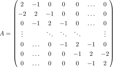
Example 2.2.4. Here we show the affine Cartan matrix and corresponding Dynkin diagram associated with the affine Lie algebra g =Bn(1). The rows and columns of the Cartan matrix
correspond to then+ 1 node, starting with row (or column) 0 and ending with row (or column) n. Notice that the second node is connected to the 0th, 1st, and 3rd node, as indicated by the corresponding a2i =ai2 entries. The n−1st and nth node are connected by two edges, since an,n−1 =−2 with an arrow across the edges pointing toward thenth node.
2 0 −1 0 0 . . . 0 0 2 −1 0 0 . . . 0 −1 −1 2 −1 0 . . . 0 0 0 −1 2 −1 . . . 0 ..
. . .. ...
0 . . . 0 0 −1 2 −1 0 . . . 0 0 0 −2 2
· · ·
2 1
1
2 2 2
Arealizationof an (n+1)×(n+1) affine Cartan matrixAis a triple (h,Π,Πˇ) whereh, called theCartan subalgebra, is a complex vector space of dimensionn+ 2, Π ={α0, α1, . . . , αn} ⊂h∗,
and Πˇ = {h0, h1, . . . , hn} ⊂ h such that Π and Πˇ are linearly independent and hhi, αji =
αj(hi) =aij. LetI ={0,1, . . . , n} be the index set. Following the terminology from the theory
of finite-dimensional Lie algebras, Π is the set ofsimple roots and Πˇ the set ofsimple coroots. Then Q=Pn
i=0Zαi is called the root lattice. We also designate Q+ =Pni=0Z≥0αi. With this
notation, we have the partial ordering≥ onh∗ that λ≥µ ifλ−µ∈Q+.
Definition 2.2.5. Let A be an affine Cartan matrix and let (h,Π,Πˇ) be a realization of A. Then the associated affine Lie algebra, g has generators ei, fi (i ∈ I) and h satisfying the
following conditions.
• [ei, fj] =δijhi for i, j∈I,
• [h, h0] = 0 for all h, h0∈h, • [hi, ej] =aijej fori, j∈I,
• (ad(ei))1−aijej = 0 fori6=j,
• (ad(fi))1−aijfj = 0 for i6=j.
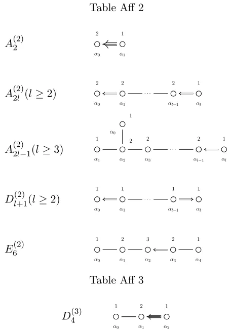
For convenience, we reproduce the tables of Dynkin diagrams associated with all affine Lie algebras from [12]. We give the corresponding Cartan matrix for each affine Lie algebra in the respective section of Chapter 3.
Table Aff 1
A(1)1
1 1
A(1)l (l≥2) · · ·
1
1 1 1 1
Bl(1)(l≥3) · · ·
1
1 2 2 2 2
Cl(1)(l≥2) · · ·
1 2 2 1
Dl(1)(l≥4) · · ·
1
1 2 2 2
1
1
G(1)2
1 2 3
F4(1)
1 2 3 4 2
E6(1)
1
1
2
2 3 2 1
E7(1)
1 2
2
3 4 3 2 1
E8(1)
Table Aff 2
A(2)2
2
α0
1
α1
A(2)2l (l≥2) · · ·
2
α0
2
α1 αl−1
2 1
αl
A(2)2l−1(l≥3) · · ·
1 α0 1 α1 2 α2 2 α3 2
αl−1
1
αl
Dl(2)+1(l≥2) · · ·
1
α0
1
α1
1
αl−1
1
αl
E6(2)
1 α0 2 α1 3 α2 2 α3 1 α4
Table Aff 3
D(3)4
1 α0 2 α1 1 α2
Given an affine Lie algebra g, letai be the labeling of the nodes in each Dynkin diagram.
a∨i is the labeling in the diagram of the corresponding dual algebra, which is found by reversing all arrows in the Dynkin diagram ofg. For example, ifg=Bn(1), then its dual algebra isA(2)2n−1. Notice if uis the vector with entries ai then Au= 0 where Ais the associated Cartan matrix.
For example, in the case g=Bn(1):
Au=
2 0 −1 0 0 . . . 0 0 2 −1 0 0 . . . 0 −1 −1 2 −1 0 . . . 0 0 0 −1 2 −1 . . . 0
..
. . .. ... ... ... ... 0 . . . 0 0 −1 2 −1 0 . . . 0 0 0 −2 2
1 1 2 2 .. . 2 2 = 0 0 0 0 .. . 0 0
As in the finite case, an important subalgebra ofgis the Cartan subalgebra,h. For everyα∈Q we associate a root space, gα = {x ∈g |[h, x] = α(h)x for all h ∈h}. Then α 6= 0 is called a
root ifgα6= 0. Associated with gis its Weyl group,W.W is the subgroup ofGL(h∗) generated by the following reflections onh∗.
The ri are called thefundamental reflections [12].
The center of g is one dimensional and is spanned by the canonical central element c =
Pn
i=0a∨ihi. Becausegis affine, by Theorem 5.6 in [12], which establishes the presence of
imag-inary roots in affine Lie algebras, we have thenull root δ =Pn
i=0aiαi ∈Q. A rootα is called
imaginary if there does not exist a w ∈W such that w(α) is a simple root. Every imaginary root in g is a nonzero integer multiple of δ. Finally, we have the derivation d ∈ h such that hαi, di= 0 for i= 1, . . . , n and hα0, di= 1.
We now have all components necessary to define the nondegenerate symmetric bilinear form (· | ·) onh:
(hi|hj) = aa∨j
jaij i, j
∈I, (hi|d) = 0 i= 1, . . . , n,
(h0|d) =a0, (d|d) = 0.
This can be extended to a bilinear form ongby defining Λ0∈h∗ by hΛ0, hii=δ0i fori∈I and
hΛ0, di= 0. With Λ0,{α0, . . . , αn,Λ0}forms a basis ofh∗ and so we define the extension of the bilinear form on gusing this basis:
(αi|αj) = a∨
i
aiaij i, j∈I
(αi|Λ0) = 0 i= 1, . . . , n
(α0|Λ0) = a10 (Λ0|Λ0) = 0
Finally, we define theuniversal enveloping algebra,U(g), to which we will return in Chapter 4. Let U(g) be an associative algebra together with a Lie algebra homomorphism j:g→ U(g) satisfying the following universal property. If (A, φ) is any pair whereAis an associative algebra andφis a Lie algebra homomorphism (φ:g→A) then there exists a unique associative algebra homomorphism ψsuch that ψj=φ. This is shown in the following diagram.
g U(g)
A
j
φ ψ
2.2.1 Integrable Highest Weight Modules
index set I ={0,1, . . . , n}, and Cartan subalgebrah. Itsweight lattice is P ={λ∈h∗ | hλ, hii ∈Zfor i∈I}.
Elements of the weight lattice are calledintegral weights. The dual weight lattice,P∨ has basis {hi ∈I} ∪ {d}. P+ = {λ ∈P | hλ, hii ≥ 0 for i∈ I} is the set of dominant integral weights.
Recall that since hαj, hii = aij ∈ Z, the root lattice, Q is contained within P. We have the
fundamental weights Λi fori= 0,1, . . . , ndefined by Λi(hj) =δij. We define thelevel,k,of any
λ∈h∗ byk=hλ, ci=Pn i=0a
∨
iλ(hi) wherec is the canonical central element.
Recall that V is a g-module if the following conditions hold for all x, y ∈ g, v, w ∈ V and a, b∈F:
• (ax+by)·v=a(x·v) +b(y·v), • x·(av+bw) =a(x·v) +b(x·w), • [x, y]·v=x·y·v−y·x·v.
Definition 2.2.6. A g-moduleV is aweight module if it admits a weight space decomposition V =⊕µ∈h∗Vµ whereVµ={v∈V|h·v=µ(h)v ∀h∈h}.µ∈h∗ is called a weight ifVµ6={0}.
In particular, we are interested in integrable highest weight modules.
Definition 2.2.7. A weight module is a highest weight module with highest weight λ, denoted V(λ), if there existsvλ 6= 0 inV(λ) such that
• U(g)·vλ =V,
• ei·vλ = 0 for all i∈I,
• h·vλ =λ(h)vλ for all h∈h.
Definition 2.2.8. A weight moduleV ofg is called integrable ifei andfi fori∈I are locally
nilpotent. That is, for everyv∈V and i∈I, there exists anN ∈Ndependent on vand isuch thateNi v= 0 and fiNv= 0.
We use the following important fact:
Lemma 2.2.9 ( [12]). Theg-moduleV(Λ) is integrable if and only if Λ∈P+.
For Λ∈P+there exists a unique (up to isomorphism) irreducible, integrable highest weight module V(Λ) generated by a highest weight vector vΛ.
Fix Λ∈P+. LetP(Λ) be the set of all weights ofV(Λ). Ifλ∈P(Λ) thenλ= Λ−Pn i=0biαi
wherebi ∈Z≥0.
Then according to [12],
P(Λ) = [
λ∈max(Λ)
{λ−nδ|n∈Z+}.
Chapter 3
Maximal Dominant Weights of
V
(
k
Λ
0
)
3.1
Introduction
In the following, we will go through each affine Lie algebragand give the corresponding index set and affine Cartan matrixA. Unless otherwise stated, we have the following notation. LetP, P∨ be the weight lattice and dual weight lattice respectively andP+ ={λ∈P|λ(hi)≥0 for all i∈
I} the set of dominant integral weights. For Λ∈P+,V(Λ) is the integrable highest weight g -module of levelk= Λ(c). We know that for any µ∈h∗ to be a weight ofV(Λ), we must have that the corresponding weight space, V(Λ)µ={v∈V(Λ) |h·v=µ(h)v, for all h∈h} 6={0}.
Thenµis of the form µ= Λ−P
i∈Ibiαi wherebi ∈Z≥0 for alli∈I and we say thatµ∈P(Λ)
whereP(Λ) is the set of all weights ofV(Λ).
A weight λ ∈ V(Λ) is called a maximal weight if λ+δ is not a weight of V(Λ). We call the set of all maximal weights of V(Λ), max(Λ). This set is important in describing the set of all weights of V(Λ) because P(Λ) = S
λ∈max(Λ){λ−nδ | n ∈ Z≥0}. That is, the set of all maximal weights is like the top of a jellyfish, with all the other weights ofV(Λ) coming off those maximal weights in strings, or tentacles. If we can describe the set of all maximal weights, then we have a description for the set of all weights. Note that any λ∈max(Λ) is W-conjugate to some maximal dominant weight, orµ∈max(Λ)∩P+, whereW is the Weyl group of the affine Lie algebra g. Then we need only describe these maximal dominant weights and wish to do so explicitly. To do so, we need to introduce a map . First, ˚his the linear span of h1, . . . , hn over C (while ˚hR is the same notion over R.) The duals, ˚h
∗ and ˚h∗
R, are defined similarly. Then for
any subsetS ofh∗, we have its orthogonal projectionS on ˚h∗ and the following formula for the map:
λ=λ− hλ, ciΛ0+ (λ|Λ0)δ whereλ∈h∗ Now we can use Proposition 12.6 in [12]:
In particular, the set of dominant maximal weights of V(Λ) is finite.
Therefore, we can find the setkCaf∩(Λ +Q) and use the inverse of the orthogonal projection
map − to determine the set of maximal dominant weights of V(Λ). We focus specifically on the integrable highest weight module V(kΛ0), of levelk. From Kac [12], we know thatkCaf =
{λ ∈˚h∗
R|λ(hi) ≥ 0 for all i ∈ I,(λ|θ) ≤ k}. Therefore, to find all maximal dominant weights
of V(Λ), we need only solve those defining inequalities. Let λ be a weight of V(Λ). Then λ= Λ−Pn
i=0biαi=kΛ0−Pni=0biαi where bi∈Z≥0 for all i∈I. Then
λ=kΛ0−
n X
i=0 biαi
=kΛ0−
n X
i=0
biαi− hkΛ0− n X
i=0
biαi, ciΛ0−(kΛ0− n X
i=0
biαi|Λ0)δ
=−
n X
i=0
biαi+b0(
n X
i=0 aiαi)
=
n X
i=1
(aib0−bi)αi
For convenience, we represent eachλ∈kCaf with ann-tuplexλ= (x1, x2, . . . , xn)∈Zn≥0where xi =aib0−bi. The defining inequalities can then be described succinctly as
˚
Ax ≥0 (λ|θ) ≤k
where ˚A is the n×n matrix obtained by removing row 0 and column 0 from A. Note that (λ|θ)≤kwill have different manifestations in the xvectors for different affine Lie algebras.
We will find all solutions to the set of defining inequalities for each type in terms of x and then use the definition of each xi to find all maximal dominant weights of V(kΛ0). Before we find the solutions, we can make a few observations about the system of inequalities. We know that xi ∈Z for all i ∈I since the xi are linear combinations of the bi. Because ˚A is of finite
type, by Theorem 4.3 in [12], which was presented in Chapter 2, then ˚Ax ≥ 0 implies that
x>0 or x= 0. Then x= 0 is one solution, though we will concern ourselves with finding the nontrivial solutions.
3.2
Type
A
(1)nmatrix A=
2 −1 0 0 . . . −1 −1 2 −1 0 . . . 0
0 −1 2 −1 . . . 0 ..
. . .. ... ... ... 0 . . . 0 −1 2 −1 −1 . . . 0 0 −1 2
.
Jayne and Misra explicitly determined the maximal dominant weights for the integrable highest weight modulesV((k−1)Λ0+ Λs),0≤s≤n, k≥2 and so for our case, we takes= 0.
In this case, the defining inequalities are
˚
Ax ≥0 x1+xn ≤k
or
2x1−x2 ≥0
−x1+ 2x2−x3 ≥0 ..
. ...
−xn−2+ 2xn−1−xn ≥0
−xn−1+ 2xn ≥0
x1+xn ≤k
where xi =b0−bi. Jayne and Misra showed that the x vectors follow a particular pattern in
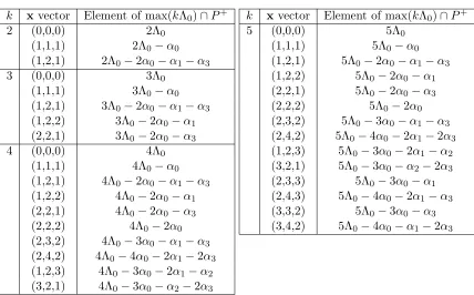
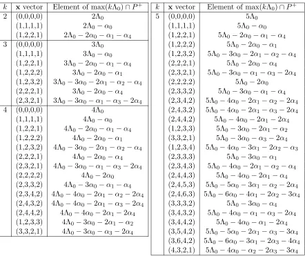
this case. As the entries inx move from left to right, they increase to a maximum element, l. The value of l may repeat in the entries, and then the entries decrease from l moving to the end of the vector. We list some examples of x vectors and corresponding maximal dominant weights in tables 3.1, 3.2, and 3.3.
3.3
Type
B
n(1)Table 3.1: xvectors and maximal dominant weights for g=A(1)2 k xvector Element of max(kΛ0)∩P+
2 (0,0) 2Λ0
(1,1) 2Λ0−α0
3 (0,0) 3Λ0
(1,1) 3Λ0−α0
(2,1) 3Λ0−2α0−α2 (1,2) 3Λ0−2α0−α1
4 (0,0) 4Λ0
(1,1) 4Λ0−α0
(2,1) 4Λ0−2α0−α2 (1,2) 4Λ0−2α0−α1
(2,2) 4Λ0−2α0
5 (0,0) 5Λ0
(1,1) 5Λ0−α0
(2,1) 5Λ0−2α0−α2 (1,2) 5Λ0−2α0−α1
(2,2) 5Λ0−2α0
(3,2) 5Λ0−3α0−α2 (2,3) 5Λ0−3α0−α1
Table 3.2: xvectors and maximal dominant weights for g=A(1)3
k x vector Element of max(kΛ0)∩P+
2 (0,0,0) 2Λ0
(1,1,1) 2Λ0−α0
(1,2,1) 2Λ0−2α0−α1−α3
3 (0,0,0) 3Λ0
(1,1,1) 3Λ0−α0
(1,2,1) 3Λ0−2α0−α1−α3 (1,2,2) 3Λ0−2α0−α1 (2,2,1) 3Λ0−2α0−α3
4 (0,0,0) 4Λ0
(1,1,1) 4Λ0−α0 (1,2,1) 4Λ0−2α0−α1−α3 (1,2,2) 4Λ0−2α0−α1 (2,2,1) 4Λ0−2α0−α3
(2,2,2) 4Λ0−2α0
(2,3,2) 4Λ0−3α0−α1−α3 (2,4,2) 4Λ0−4α0−2α1−2α3 (1,2,3) 4Λ0−3α0−2α1−α2 (3,2,1) 4Λ0−3α0−α2−2α3
k x vector Element of max(kΛ0)∩P+
5 (0,0,0) 5Λ0
(1,1,1) 5Λ0−α0
Table 3.3: xvectors and maximal dominant weights for g=A(1)4
k xvector Element of max(kΛ0)∩P+
2 (0,0,0,0) 2Λ0
(1,1,1,1) 2Λ0−α0 (1,2,2,1) 2Λ0−2α0−α1−α4
3 (0,0,0,0) 3Λ0
(1,1,1,1) 3Λ0−α0 (1,2,2,1) 3Λ0−2α0−α1−α4 (1,2,2,2) 3Λ0−2α0−α1 (1,2,3,2) 3Λ0−3α0−2α1−α2−α4 (2,2,2,1) 3Λ0−2α0−α4 (2,3,2,1) 3Λ0−3α0−α1−α3−2α4
4 (0,0,0,0) 4Λ0
(1,1,1,1) 4Λ0−α0 (1,2,2,1) 4Λ0−2α0−α1−α4 (1,2,2,2) 4Λ0−2α0−α1 (1,2,3,2) 4Λ0−3α0−2α1−α2−α4 (2,2,2,1) 4Λ0−2α0−α4 (2,3,2,1) 4Λ0−3α0−α1−α3−2α4 (2,2,2,2) 4Λ0−2α0
(2,3,3,2) 4Λ0−3α0−α1−α4 (2,3,4,2) 4Λ0−4α0−2α1−α2−2α4 (2,4,3,2) 4Λ0−4α0−2α1−α3−2α4 (2,4,4,2) 4Λ0−4α0−2α1−2α4 (1,2,3,3) 4Λ0−3α0−2α1−α2 (3,3,2,1) 4Λ0−3α0−α3−2α4
k x vector Element of max(kΛ0)∩P+
5 (0,0,0,0) 5Λ0
(1,1,1,1) 5Λ0−α0
(1,2,2,1) 5Λ0−2α0−α1−α4 (1,2,2,2) 5Λ0−2α0−α1 (1,2,3,2) 5Λ0−3α0−2α1−α2−α4 (2,2,2,1) 5Λ0−2α0−α4 (2,3,2,1) 5Λ0−3α0−α1−α3−2α4 (2,2,2,2) 5Λ0−2α0
Cartan matrix A=
2 0 −1 0 0 . . . 0 0 2 −1 0 0 . . . 0 −1 −1 2 −1 0 . . . 0 0 0 −1 2 −1 . . . 0
..
. . .. ... ... ... ... 0 . . . 0 0 −1 2 −1 0 . . . 0 0 0 −2 2
.
The defining inequalities are equivalent to
˚ Ax≥0 x2 ≤k
wherex1=b0−b1 and xi = 2b0−bi for 2≤i≤n. That is,
2x1−x2 ≥0
−x1+ 2x2−x3 ≥0 −x2+ 2x3−x4 ≥0
..
. ...
−xn−3+ 2xn−2−xn−1 ≥0 −xn−2+ 2xn−1−xn ≥0
−2xn−1+ 2xn ≥0
x2 ≤k
Recall that we are looking for the nontrivial solutions, x > 0. Note as well that this means b0 > b1 andb0 > b2i for 2≤i≤n.
Lemma 3.3.1. Let x be a solution to
˚ Ax≥0 x2≤k
Then xi ≤xi+1 for 1≤i≤n−1. In addition, xi−xi−1 ≥xi+1−xi.
Proof. Assume, for the sake of contradiction, that there exists a 2≤j≤nsuch thatxj < xj−1. If j 6= n, then since −xj−1 + 2xj −xj+1 ≥ 0, we have xj −xj+1 ≥ xj−1 −xj > 0 by our
−xi−1+ 2xi−xi+1≥0, implying that xi−xi−1≥xi+1−xi. Lemma 3.3.2. The set of solutions to
˚ Ax≥0 x2≤k
is
{x=0} ∪ {x= (x1, x2, . . . , xn)∈Zn≥0 |1≤x2≤k, x1=lx2
2
m
+l1,0≤l1 ≤jx2 2
k
,
xi=x2+
i X
j=3 lj,
0≤l3 ≤
jx2
2
k
−l1,0≤ln≤ln−1 ≤ln−2≤ · · · ≤l4 ≤l3 for all 3≤i≤n}.
Proof. As stated above, since ˚Ais of finite type,x>0 orx= 0 and sox2= 0 gives the solution
x= 0. Now, fix x2 such that 1≤x2 ≤k. Then by ( ˚Ax)1 ≥0, x1 ≥ x22. Since eachxi must be
an integer, this implies x1 ≥ x2
2
. We have observed that the first n coordinates of x do not decrease, therefore x1 ≤ x2. Then x2
2
≤ x1 ≤x2 and so we can write x1 = x2
2
+l1 where 0≤l1 ≤
x2
2
. We will prove the pattern for the remaining coordinates by induction. First, as a base case, we show the expression forx3. Again, since the coordinates do not decrease,x2≤x3 and from the previous lemma,x3−x2 ≤x2−x1. Then x3−x2 ≤x2−(x2
2
+l1) =x2
2
−l1. Therefore, x2 ≤ x3 ≤ x2 +
x2
2
−l1 and so x3 = x2 +l3 where 0 ≤ l3 ≤
x2
2
−l1. Now, assume that xi is of the form xi = x2 +Pij=3lj for all 3 ≤ i ≤ p < n where lj = xj −xj−1 and so 0≤lp ≤lp−1 ≤ · · · ≤l4≤l3 by the second result of Lemma 3.3.1. By the same lemma, xp ≤xp+1 ≤2xp−xp−1. Applying the induction hypothesis, we have x2+Ppj=3lj ≤xp+1 ≤ 2(x2+Pp
j=3lj)−(x2+
Pp−1
j=3lj) =x2+ (
Pp
j=3lj) +lp. Thenxp+1 =x2+ (
Pp
j=3lj) +lp+1 where 0≤lp+1 ≤lp. Therefore, xi =x2+Pij=3lj where 0≤ln≤ln−1≤ · · · ≤l4 ≤l3 and so li is the
amount of increase from xi−1 toxi where 3≤i≤n.
Theorem 3.3.3. Let n ≥ 3, Λ = kΛ0, k ≥ 2. Then max(Λ)∩P+ = {Λ} ∪ {Λ−lα0−(l− (x2
2
+l1))α1−(2l−x2)α2−Pn
i=3(2l−(x2+
Pi
j=3lj))αi
where
• 1≤x2 ≤k,
• l= max{x1,
xn
2
},
• 0≤l1≤
x2
2
,
• 0≤l3≤ bx22c −l1,
Proof. By Proposition 12.6 in [12], the map λ 7→ λ is a bijection from max(Λ)∩P+ onto kCaf∩(Λ +Q). We first find all elements of kCaf∩(Λ +Q) and use this bijection to then find
all elements of max(Λ)∩P+. By definition,
kCaf∩(Λ +Q) ={λ∈˚h∗R|λ(hi)≥0 for alli∈˚I,(λ|θ)≤k}.
We found the set of solutions to these inequalities in Lemma 3.3.2. Recall that by the bijection, λ= Λ−Pn
i=0biαi ∈max{Λ} ∩P+, withbi ∈Z≥0 for all 0≤i≤n, maps toλ=Pni=1xiαi ∈
kCaf ∩(Λ +Q). The map gives that x1 = b0−b1 and xi = 2b0 −bi for 2 ≤ i ≤ n. Then
(b0, b1, . . . , bn) = (b0, b0−x1,2b0−x2, . . . ,2b0−xn). Then if we can determineb0, we will have
the set of all maximal dominant weights since we have already found the pattern for all xi. By
definition, thebi ≥0 for 0≤i≤n. Therefore, the following must be true:
b0 ≥0 b0−x1 ≥0 2b0−x2 ≥0
.. . 2b0−xn≥0
It is clear that b0 ≥ x1 where x1 = (
x2
2
+l1). We have already proven that the first n coordinates ofxnever decrease. Therefore,xn= max1≤i≤n{xi}and so for the inner inequalities
it is sufficient to say that b0 ≥ xn
2 . Since xn may be odd and the bi are integers, we need b0 ≥
xn
2
. Then let l = max{x1,
xn
2
} and so b0 ≥ l. We claim that b0 = l. For the sake of contradiction, suppose b0=l+r wherer ∈Z>0. Then
λ+δ= Λ−(l+r−1)α0−(l+r−x1−1)α1−(2l+ 2r−x2−2)α2− · · · −(2l+ 2r−xn−2)αn.
Then if each of the subtracted coefficients of the αi,0 ≤i ≤ n is greater than or equal to 0,
we will have λ+δ ≤Λ andλ+δ ∈P+. First, l+r−1 ≥0 sincel ≥x1 ≥1 and we assume r >0 then l+r−1 >0. Second, since l≥x1 and r ≥1 we have l+r−x1−1 ≥0. Finally, since l ≥ xn
2
, we have 2l ≥ 2xn
2
which means 2l ≥ xn if xn is even or 2l ≥ xn+ 1 if xn
is odd. Either way, 2l ≥ xn ≥ xi for all 2 ≤ i ≤ n. Since r ≥ 1 then 2r ≥ 2 and we have
2l+ 2r−xi−2≥0 for all 2≤i≤n. Then λ+δ is a weight of V(Λ) which contradicts that
λ∈max{Λ}. Therefore,r = 0 andλ= Λ−lα0−(l−x1)α1−(2l−x2)α2− · · · −(2l−xn)αn.
Combining this with our solutions for the xi from Lemma 3.3.2, we have the pattern given
above.
Table 3.4: x vectors and maximal dominant weights for theg=B5(1)-moduleV(2Λ0) x2 l1, l3, l4, l5 x vector l Element of max(3Λ0)∩P+
0 0,0,0,0 (0,0,0,0,0) 0 2Λ0
1 0,0,0,0 (1,1,1,1,1) 1 2Λ0−α0−α2−α3−α4−α5
2 0,0,0,0 (1,2,2,2,2) 1 2Λ0−α0
2 0,1,0,0 (1,2,3,3,3) 2 2Λ0−2α0−α1−2α2−α3−α4−α5 2 0,1,1,0 (1,2,3,4,4) 2 2Λ0−2α0−α1−2α2−α3 2 0,1,1,1 (1,2,3,4,5) 3 2Λ0−3α0−2α1−4α2−3α3−2α4−α5 2 1,0,0,0 (2,2,2,2,2) 2 2Λ0−2α0−2α2−2α3−2α4−2α5
Note thatXl,n⊆Xk,n whenever l≤k.
Example 3.3.4. B5(1), V(Λ) =V(2Λ0). Using the theorem, we have that max(2Λ0)∩P+={2Λ0} ∪ {2Λ0−lα0−(l−(lx2
2
m
+l1))α1−(2l−x2)α2−(2l−(x2+l3))α3 −(2l−(x2+l3+l4))α4−(2l−(x2+l3+l4+l5))α5}. Since 1 ≤ x2 ≤ k and k = 2, then we have x2 = 1 or x2 = 2. First, consider x2 = 1. Then 0 ≤l1 ≤x2
2
= 0. Then l1 = 0 and so x1 =x2
2
+ 0 = 1 and 0≤ l3 ≤ 0. This implies that l4 = l5 = 0. Therefore, we obtain the x vector (1,1,1,1,1). Then l = 1, giving the maximal dominant weight 2Λ0−α0−α2−α3−α4−α5.
The only choice we made (and so the only value we can change) was that for x2. Then consider x2 = 2. This implies that 0≤ l1 ≤1. Once more, we have a choice. First, let l1 = 0. Then x1 = 1 and 0≤l3 ≤1. First, choose l3 = 0, which implies that l4 =l5 = 0. This gives the x vector (1,2,2,2,2). By the theorem, this corresponds to the maximal dominant weight 2Λ0 −α0 since l = 1 = x1 =
x5 2
. Next, we consider l3 = 1. Then 0 ≤ l5 ≤ l4 ≤ 1. We choose l4 = 0, which implies l5 = 0. This gives the x vector (1,2,3,3,3), and so l =3
2
= 2. The resulting maximal dominant weight is 2Λ0 −2α0−α1 −2α2−α3−α4 −α5. If l4 = 1, then l5 = 0 or l5 = 1. l5 = 0 gives the x vector (1,2,3,4,4) and l5 = 1 gives the x vector (1,2,3,4,5). The corresponding maximal dominant weights are 2Λ0 −2α0 −α1 −2α2 −α3 and 2Λ0 −3α0 −2α1 −4α2 −3α3 −2α4 −α5 respectively. We have exhausted all possible choices for l1 = 0. Now, consider l1 = 1. Then 0 ≤ l3 ≤
2
2
−1 = 0, which implies that l3 = l4 = l5 = 0. This gives the x vector (2,2,2,2,2) with corresponding maximal dominant weight 2Λ0−2α0 −2α2−2α3 −2α4−2α5. We list these results in Table 3.4. One can check that this set corresponds to that of [18],
Table 3.5: x vectors and maximal dominant weights for theg=B6(1)-moduleV(2Λ0) x2 l1, l3, l4, l5, l6 x vector l Element of max(3Λ0)∩P+
0 0,0,0,0,0 (0,0,0,0,0,0) 0 2Λ0
1 0,0,0,0,0 (1,1,1,1,1,1) 1 2Λ0−α0−α2−α3−α4−α5−α6 2 0,0,0,0,0 (1,2,2,2,2,2) 1 2Λ0−α0
2 0,1,0,0,0 (1,2,3,3,3,3) 2 2Λ0−2α0−α1−2α2−α3−α4−α5−α6 2 0,1,1,0,0 (1,2,3,4,4,4) 2 2Λ0−2α0−α1−2α2−α3
2 0,1,1,1,0 (1,2,3,4,5,5) 3 2Λ0−3α0−2α1−4α2−3α3−2α4−α5−α6 2 0,1,1,1,1 (1,2,3,4,5,6) 3 2Λ0−3α0−2α1−4α2−3α3−2α4−α5 2 1,0,0,0,0 (2,2,2,2,2,2) 2 2Λ0−2α0−2α2−2α3−2α4−2α5−2α6
Example 3.3.5. B6(1), V(Λ) =V(2Λ0). By the theorem, we have max(2Λ0)∩P+={2Λ0} ∪ {2Λ0−lα0−(l−(lx2
2
m
+l1))α1−(2l−x2)α2−(2l−(x2+l3))α3 −(2l−(x2+l3+l4))α4−(2l−(x2+l3+l4+l5))α5
−(2l−(x2+l3+l4+l5+l6))α6}.
x2 = 1 : Then 0≤l1 ≤0 and so 0≤l3 ≤0−0, implying l1 =l3 =· · ·=l6 = 0 giving thex vector (1,1,1,1,1,1) with corresponding maximal dominant weight 2Λ0−α0−α2−α3−α4− α5−α6.
x2 = 2 :Then 0≤l1 ≤1.
Consider l1= 0. Thenx1= 1 and 0≤l3 ≤1.
First, consider l3 = 0. Then x3 = x2 = 2 and 0 ≤ l6 ≤ l5 ≤ l4 ≤ 0. This gives the x vector (1,2,2,2,2,2) with corresponding maximal dominant weight 2Λ0−α0.
Now considerl3= 1. Then x3 = 3 and 0≤l6 ≤l5 ≤l4≤1.
Ifl4= 0, we obtain thexvector (1,2,3,3,3,3) with corresponding maximal dominant weight 2Λ0−2α0−α1−2α2−α3−α4−α5−α6.
If l4 = 1 and l5 = 0, we obtain the x vector (1,2,3,4,4,4) with corresponding maximal dominant weight 2Λ0−2α0−α1−2α2−α3.
If l4 = l5 = 1 and l6 = 0, we have (1,2,3,4,5,5) with maximal dominant weight 2Λ0−3α0−2α1−4α2−3α3−2α4−α5−α6.
If l4 = l5 = l6 = 1, we have (1,2,3,4,5,6) with maximal dominant weight 2Λ0− 3α0−2α1−4α2−3α3−2α4−α5.
Finally, considerl1 = 1. Then 0≤l3≤0 implies that 0 =l3=l4=l5 =l6. This gives thex
vector and maximal dominant weight (2,2,2,2,2,2) and 2Λ0−2α0−2α2−2α3−2α4−2α5−2α6. We list these results in Table 3.5.
into sets according to level, in the case ofk= 2 to the following:
max(2Λ0)∩P+ ={2Λ0} ∪ {2Λ0−α0−
n X
i=2 αi}
∪ {2Λ0−lα0−(l−(1 +l1))α1−(2l−2)α2−(
n X
i=3
(2l−(2 +
i X
j=3
lj))αi)}
According to [18], the set of maximal dominant weights for V(2Λ0) is
{(1 +δ2u−1,n)Λ2u−1−uδ |2≤u≤
n+ 1 2
} ∪ {(1 +δ2u,n)Λ2u−uδ|1≤u≤ jn
2
k
}
∪ {Λ0+ Λ1−δ} ∪ {2Λ0,2Λ1−2δ}.
To prove that the two formulations are the same, we first write our formulation in terms of the fundamental dominant weights, Λi. Note that we must use the entries of the Cartan matrix
corresponding to A(2)2n−1 as the coefficients of the Λi, in order to satisfy thatPni=0aiαi=δ and
αj(hi) =aij. We have the following:
α0= 2Λ0−Λ2+δ α1= 2Λ1−Λ2
α2=−Λ0−Λ1+ 2Λ2−Λ3 α3=−Λ2+ 2Λ3−Λ4
.. .
αn−1=−Λn−2+ 2Λn−1−2Λn
αn=−Λn−1+ 2Λn
Then our formulation becomes:
X={2Λ0} ∪ {2Λ0−(2Λ0−Λ2+δ)−(−Λ0−Λ1+ 2Λ2−Λ3) −
n−2
X
i=3
(−Λi−1+ 2Λi−Λi+1)
−(−Λn−2+ 2Λn−1−2Λn)−(−Λn−1+ 2Λn)}
∪ {2Λ0−l(2Λ0−Λ2+δ)−(l−(1 +l1))(2Λ1−Λ2)−(2l−2)(−Λ0−Λ1+ 2Λ2−Λ3) −
n−2
X
i=3
(2l−(2 +
i X
j=3
lj))(−Λi−1+ 2Λi−Λi+1)
−(2l−(2 +
n−1
X
j=3
lj))(−Λn−2+ 2Λn−1−2Λn)
−(2l−(2 +
n X
j=3
We now show that
X ={(1 +δ2u−1,n)Λ2u−1−uδ |2≤u≤
n+ 1 2
} ∪ {(1 +δ2u,n)Λ2u−uδ |1≤u≤ jn
2
k
}
∪ {Λ0+ Λ1−δ} ∪ {2Λ0,2Λ1−2δ}
2Λ0 is included in both sets so we move on to the remaining weights. Consider the level 1 weight 2Λ0−(2Λ0−Λ2+δ)−(−Λ0−Λ1+ 2Λ2−Λ3)−Pn−2
i=3(−Λi−1+ 2Λi−Λi+1)−(−Λn−2+ 2Λn−1−2Λn)−(−Λn−1+ 2Λn). We immediately see that we have Λ0+ Λ1−δcoming from the first three summands. One can check that all other terms cancel, leaving us with Λ0+ Λ1−δ, matching another of the weights in [18].
We now consider the general term in our expression forW. Sincex2= 2,l1 can be 0 or 1. If l1 = 1, this implies thatln=ln−1=· · ·=l3 = 0 which gives thexvector (2,2, . . . ,2), meaning l= 2. Simplifying the general expression, we obtain 2Λ0−2(2Λ0−Λ2+δ)−2(−Λ0−Λ1+ 2Λ2− Λ3)−Pni=3−22(−Λi−1+ 2Λi−Λi+1)−2(−Λn−2+ 2Λn−1−2Λn)−2(−Λn−1+ 2Λn). Simplifying
this further, we obtain 2Λ1−2δ, completing the fourth set in the description in [18].
Now consider if l1 = l3 = 0. This implies ln = ln−1 = · · · = l4 = l3 = 0, giving x vector (1,2, . . . ,2). In this case,l= 1 and we consider our general term once more: 2Λ0−(2Λ0−Λ2+δ) = Λ2−δ. This corresponds to the weight in second set for [18] where u= 1.
Finally, we consider the remaining weights. Letl1 = 0 andkbe the smallest integer between 4 and n such that lk = 0. This implies l3 =l4 =· · · =lk−1 = 1 and lk =lk+1 =· · · =ln = 0.
Then since l = max{x1,xn
2
} and the x vector is nondecreasing by Lemma 3.3.1, l =k−1
2
. Then our general expression becomes
2Λ0−
k−1 2
(2Λ0−Λ2+δ)−
k−1 2
−1(2Λ1−Λ2) −2
k−1 2
−2(−Λ0−Λ1+ 2Λ2−Λ3)
−
k−1
X
i=3
2
k−1 2
−(2 +
i X
j=3
1)(−Λi−1+ 2Λi−Λi+1)
−
n−2
X
i=k
2
k−1 2
−(2 +
k−1
X
j=3
1)(−Λi−1+ 2Λi−Λi+1)
−2
k−1 2
−(2 +
k−1
X
j=3
1)(−Λn−2+ 2Λn−1−2Λn)
−2
k−1 2
−(2 +
k−1
X
j=3
1)(−Λn−1+ 2Λn)
−
k−1
X
i=3
(k−1−(2 +
i X
j=3
1))(−Λi−1+ 2Λi−Λi+1)
−
n−2
X
i=k
(k−1−(2 +
k−1
X
j=3
1))(−Λi−1+ 2Λi−Λi+1)
−(k−1−(2 +
k−1
X
j=3
1))(−Λn−2+ 2Λn−1−2Λn)−(k−1−(2 + k−1
X
j=3
1))(−Λn−1+ 2Λn)
Collecting like terms, we have
2Λ0−(k−1)Λ0+ (k−3)Λ0−(k−3)Λ1+ (k−3)Λ1 +k−1
2 Λ2+ k−3
2 Λ2−2(k−3)Λ2+ (k−4)Λ2 +
k−2
X
i=3
(k−i)Λi−2(k−(i+ 1))Λi+ (k−(i+ 2))Λi
+ Λk−1− k−1
2 δ = Λk−1−
k−1 2 δ
This corresponds to the second set we have listed except for whenu=n
2
andnis even. Notice we have also left out the case in which nis even and lk= 1 for all 3≤k≤n. These two cases
correspond as we show below. In this situation,l= max{x1,xn
2
}= max{1,n
2}=
n
2. 2Λ0−n
2(2Λ0−Λ2+δ)−
n
2 −1
(2Λ1−Λ2)−(n−2)(−Λ0−Λ1+ 2Λ2−Λ3) −
n−2
X
i=3
(n−(2 +
i X
j=3
1))(−Λi−1+ 2Λi−Λi+1)−(n−(2 + n−1
X
j=3
1))(−Λn−2+ 2Λn−1−2Λn)
−(n−(2 +
n X
j=3
1))(−Λn−1+ 2Λn)
Collecting like terms, this becomes
2Λ0−nΛ0+ (n−2)Λ0−(n−2)Λ1+ (n−2)Λ1 +n
2Λ2+ ( n
2 −1)Λ2−2(n−2)Λ2+ (n−3)Λ2 +
n−1
X
i=3
(n−(i−1))Λi−2(n−i)Λi+ (n−(i+ 1))Λi
+ 2Λn−
n 2δ = 2Λn−
n 2δ
such thatlk= 0:
2Λ0−k
2(2Λ0−Λ2+δ)−( k
2 −1)(2Λ1−Λ2)−(k−2)(−Λ0−Λ1+ 2Λ2−Λ3) −
k−1
X
i=3
(k−(2 +
i X
j=3
1))(−Λi−1+ 2Λi−Λi+1)
−
n−2
X
i=k
(k−(2 +
k−1
X
j=3
1))(−Λi−1+ 2Λi−Λi+1)
−(k−(2 +
k−1
X
j=3
1))(−Λn−2+ 2Λn−1−2Λn)−(k−(2 + k−1
X
j=3
1))(−Λn−1+ 2Λn)
= 2Λ0−kΛ0+ (k−2)Λ0−(k−2)Λ1+ (k−2)Λ1 +k
2Λ2+ ( k
2 −1)Λ2−2(k−2)Λ2+ (k−3)Λ2 +
k−2
X
i=3
(k−(i−1))Λi−2(k−i)Λi+ (k−(i+ 1))Λi
+ 2Λk−1−2Λk−1+ Λk−1− k 2δ = Λk−1−
k 2δ
This corresponds to the first set we have listed, except for the final term whenu=n+1
2
andnis odd. This is the case whennis odd andlk= 1 for all 3≤k≤n. Thenl= max{x1,
xn
2
}= n+12 . This gives
2Λ0− n+ 1
2 (2Λ0−Λ2+δ)−( n+ 1
2 −1)(2Λ1−Λ2)−(n+ 1−2)(−Λ0−Λ1+ 2Λ2−Λ3) −
n−2
X
i=3
(n+ 1−(2 +
i X
j=3
1))(−Λi−1+ 2Λi−Λi+1)
−(n+ 1−(2 +
n−1
X
j=3
1))(−Λn−2+ 2Λn−1−2Λn)
−(n+ 1−(2 +
n X
j=3
1))(−Λn−1+ 2Λn)
= 2Λ0−(n+ 1)Λ0+ (n−1)Λ0−(n−1)Λ1+ (n−1)Λ1 +n+ 1
2 Λ2+ ( n+ 1
2 −1)Λ2−2(n−1)Λ2+ (n−2)Λ2 +
n−1
X
i=3
(n+ 1−(i−1))Λi−2(n+ 1−i)Λi+ (n+ 1−(i+ 1))Λi
+ 4Λn−2Λn−
n+ 1 2 δ = 2Λn−
Table 3.6: x vectors and maximal dominant weights for theg=B5(1)-moduleV(3Λ0) x2 l1, l3, l4, l5 x vector l Element of max(3Λ0)∩P+
0 0,0,0,0 (0,0,0,0,0) 0 3Λ0
1 0,0,0,0 (1,1,1,1,1) 1 3Λ0−α0−α2−α3−α4−α5
2 0,0,0,0 (1,2,2,2,2) 1 3Λ0−α0
2 0,1,0,0 (1,2,3,3,3) 2 3Λ0−2α0−α1−2α2−α3−α4−α5 2 0,1,1,0 (1,2,3,4,4) 2 3Λ0−2α0−α1−2α2−α3 2 0,1,1,1 (1,2,3,4,5) 3 3Λ0−3α0−2α1−4α2−3α3−2α4−α5 2 1,0,0,0 (2,2,2,2,2) 2 3Λ0−2α0−2α2−2α3−2α4−2α5 3 0,0,0,0 (2,3,3,3,3) 2 3Λ0−2α0−α2−α3−α4−α5 3 0,1,0,0 (2,3,4,4,4) 2 3Λ0−2α0−α2
3 0,1,1,0 (2,3,4,5,5) 3 3Λ0−3α0−α1−3α2−2α3−α4−α5 3 0,1,1,1 (2,3,4,5,6) 3 3Λ0−3α0−α1−3α2−2α3−α4 3 1,0,0,0 (3,3,3,3,3) 3 3Λ0−3α0−3α2−3α3−3α4−3α5
This finishes the right hand side of the equation. Therefore, the two sets are equal and our formulation matches that of [18] for k= 2.
We include several more examples for different values of k below.
Example 3.3.6. B5(1), V(Λ) =V(3Λ0). According to Theorem 3.3.3, max(Λ)∩P+={Λ} ∪ {Λ−lα0−(l−(lx2
2
m
+l1))α1−(2l−x2)α2−(2l−(x2+l3))α3 −(2l−(x2+l3+l4))α4−(2l−(x2+l3+l4+l5))α5
where 1 ≤x2 ≤ 3 and the restrictions on l and the li are as listed in the theorem statement.
We obtain the results in Table 3.6.
Example 3.3.7. B6(1), V(Λ) =V(3Λ0). According to Theorem 3.3.3, max(Λ)∩P+={Λ} ∪ {Λ−lα0−(l−(lx2
2
m
+l1))α1−(2l−x2)α2−(2l−(x2+l3))α3 −(2l−(x2+l3+l4))α4−(2l−(x2+l3+l4+l5))α5
−(2l−(x2+l3+l4+l5+l6))α6
where 1 ≤x2 ≤ 3 and the restrictions on l and the li are as listed in the theorem statement.
We obtain the results in Table 3.7.
Example 3.3.8. B5(1), V(Λ) =V(4Λ0). According to Theorem 3.3.3, max(Λ)∩P+={Λ} ∪ {Λ−lα0−(l−(lx2
2
m
+l1))α1−(2l−x2)α2−(2l−(x2+l3))α3 −(2l−(x2+l3+l4))α4−(2l−(x2+l3+l4+l5))α5
Table 3.7: x vectors and maximal dominant weights for theg=B6(1)-moduleV(3Λ0) x2 l1, l3, l4, l5, l6 x vector l Element of max(3Λ0)∩P+
0 0,0,0,0,0 (0,0,0,0,0,0) 0 3Λ0
1 0,0,0,0,0 (1,1,1,1,1,1) 1 3Λ0−α0−α2−α3−α4−α5−α6
2 0,0,0,0,0 (1,2,2,2,2,2) 1 3Λ0−α0
2 0,1,0,0,0 (1,2,3,3,3,3) 2 3Λ0−2α0−α1−2α2−α3−α4−α5−α6 2 0,1,1,0,0 (1,2,3,4,4,4) 2 3Λ0−2α0−α1−2α2−α3
2 0,1,1,1,0 (1,2,3,4,5,5) 3 3Λ0−3α0−2α1−4α2−3α3−2α4−α5−α6 2 0,1,1,1,1 (1,2,3,4,5,6) 3 3Λ0−3α0−2α1−4α2−3α3−2α4−α5 2 1,0,0,0,0 (2,2,2,2,2,2) 2 3Λ0−2α0−2α2−2α3−2α4−2α5−2α6 3 0,0,0,0,0 (2,3,3,3,3,3) 2 3Λ0−2α0−α2−α3−α4−α5−α6 3 0,1,0,0,0 (2,3,4,4,4,4) 2 3Λ0−2α0−α2
3 0,1,1,0,0 (2,3,4,5,5,5) 3 3Λ0−3α0−α1−3α2−2α3−α4−α5−α6 3 0,1,1,1,0 (2,3,4,5,6,6) 3 3Λ0−3α0−α1−3α2−2α3−α4 3 0,1,1,1,1 (2,3,4,5,6,7) 4 3Λ0−4α0−2α1−5α2−4α3−3α4−2α5−α6 3 1,0,0,0,0 (3,3,3,3,3,3) 3 3Λ0−3α0−3α2−3α3−3α4−3α5−3α6
We obtain the results in Table 3.8.
Example 3.3.9. B6(1), V(Λ) =V(4Λ0). According to Theorem 3.3.3, max(Λ)∩P+={Λ} ∪ {Λ−lα0−(l−(
lx2
2
m
+l1))α1−(2l−x2)α2−(2l−(x2+l3))α3 −(2l−(x2+l3+l4))α4−(2l−(x2+l3+l4+l5))α5
−(2l−(x2+l3+l4+l5+l6))α6
where 1 ≤x2 ≤ 4 and the restrictions on l and the li are as listed in the theorem statement.
We obtain the results in Table 3.9.
3.4
Type
C
n(1)We now considerg=Cn(1) forn≥2, index set I ={0,1, . . . , n}, and Cartan matrix
A=
2 −1 0 0 0 . . . 0 −2 2 −1 0 0 . . . 0 0 −1 2 −1 0 . . . 0
..
. . .. ... ... ... 0 . . . 0 −1 2 −1 0 0 . . . 0 0 −1 2 −2 0 . . . 0 0 0 −1 2
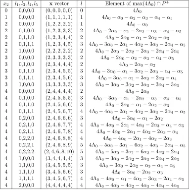
Table 3.8: x vectors and maximal dominant weights for theg=B5(1)-moduleV(4Λ0) x2 l1, l3, l4, l5 x vector l Element of max(4Λ0)∩P+
0 0,0,0,0 (0,0,0,0,0) 0 4Λ0
1 0,0,0,0 (1,1,1,1,1) 1 4Λ0−α0−α2−α3−α4−α5
2 0,0,0,0 (1,2,2,2,2) 1 4Λ0−α0
2 0,1,0,0 (1,2,3,3,3) 2 4Λ0−2α0−α1−2α2−α3−α4−α5 2 0,1,1,0 (1,2,3,4,4) 2 4Λ0−2α0−α1−2α2−α3 2 0,1,1,1 (1,2,3,4,5) 3 4Λ0−3α0−2α1−4α2−3α3−2α4−α5 2 1,0,0,0 (2,2,2,2,2) 2 4Λ0−2α0−2α2−2α3−2α4−2α5 3 0,0,0,0 (2,3,3,3,3) 2 4Λ0−2α0−α2−α3−α4−α5 3 0,1,0,0 (2,3,4,4,4) 2 4Λ0−2α0−α2
3 0,1,1,0 (2,3,4,5,5) 3 4Λ0−3α0−α1−3α2−2α3−α4−α5 3 0,1,1,1 (2,3,4,5,6) 3 4Λ0−3α0−α1−3α2−2α3−α4 3 1,0,0,0 (3,3,3,3,3) 3 4Λ0−3α0−3α2−3α3−3α4−3α5
4 0,0,0,0 (2,4,4,4,4) 2 4Λ0−2α0
4 0,1,0,0 (2,4,5,5,5) 3 4Λ0−3α0−α1−2α2−α3−α4−α5 4 0,1,1,0 (2,4,5,6,6) 3 4Λ0−3α0−α1−2α2−α3 4 0,1,1,1 (2,4,5,6,7) 4 4Λ0−4α0−2α1−4α2−3α3−2α4−α5 4 0,2,0,0 (2,4,6,6,6) 3 4Λ0−3α0−α1−2α2
4 0,2,1,0 (2,4,6,7,7) 4 4Λ0−4α0−2α1−4α2−2α3−α4−α5 4 0,2,1,1 (2,4,6,7,8) 4 4Λ0−4α0−2α1−4α2−2α3−α4 4 0,2,2,0 (2,4,6,8,8) 4 4Λ0−4α0−2α1−4α2−2α3 4 0,2,2,1 (2,4,6,8,9) 5 4Λ0−5α0−3α1−6α2−4α3−2α4−α5 4 0,2,2,2 (2,4,6,8,10) 5 4Λ0−5α0−3α1−6α2−4α3−2α4 4 1,0,0,0 (3,4,4,4,4) 3 4Λ0−3α0−2α2−2α3−2α4−2α5 4 1,1,0,0 (3,4,5,5,5) 3 4Λ0−3α0−2α2−α3−α4−α5 4 1,1,1,0 (3,4,5,6,6) 3 4Λ0−3α0−2α2−α3
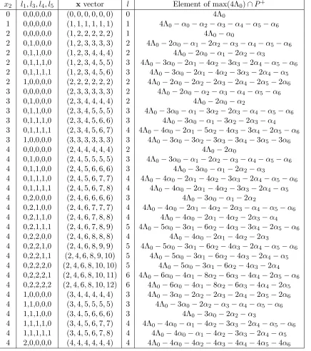
Table 3.9: x vectors and maximal dominant weights for theg=B6(1)-moduleV(4Λ0) x2 l1, l3, l4, l5 xvector l Element of max(4Λ0)∩P+
0 0,0,0,0,0 (0,0,0,0,0,0) 0 4Λ0
1 0,0,0,0,0 (1,1,1,1,1,1) 1 4Λ0−α0−α2−α3−α4−α5−α6 2 0,0,0,0,0 (1,2,2,2,2,2) 1 4Λ0−α0
2 0,1,0,0,0 (1,2,3,3,3,3) 2 4Λ0−2α0−α1−2α2−α3−α4−α5−α6 2 0,1,1,0,0 (1,2,3,4,4,4) 2 4Λ0−2α0−α1−2α2−α3
2 0,1,1,1,0 (1,2,3,4,5,5) 3 4Λ0−3α0−2α1−4α2−3α3−2α4−α5−α6 2 0,1,1,1,1 (1,2,3,4,5,6) 3 4Λ0−3α0−2α1−4α2−3α3−2α4−α5 2 1,0,0,0,0 (2,2,2,2,2,2) 2 4Λ0−2α0−2α2−2α3−2α4−2α5−2α6 3 0,0,0,0,0 (2,3,3,3,3,3) 2 4Λ0−2α0−α2−α3−α4−α5−α6 3 0,1,0,0,0 (2,3,4,4,4,4) 2 4Λ0−2α0−α2
3 0,1,1,0,0 (2,3,4,5,5,5) 3 4Λ0−3α0−α1−3α2−2α3−α4−α5−α6 3 0,1,1,1,0 (2,3,4,5,6,6) 3 4Λ0−3α0−α1−3α2−2α3−α4 3 0,1,1,1,1 (2,3,4,5,6,7) 4 4Λ0−4α0−2α1−5α2−4α3−3α4−2α5−α6 3 1,0,0,0,0 (3,3,3,3,3,3) 3 4Λ0−3α0−3α2−3α3−3α4−3α5−3α6 4 0,0,0,0,0 (2,4,4,4,4,4) 2 4Λ0−2α0
4 0,1,0,0,0 (2,4,5,5,5,5) 3 4Λ0−3α0−α1−2α2−α3−α4−α5−α6 4 0,1,1,0,0 (2,4,5,6,6,6) 3 4Λ0−3α0−α1−2α2−α3
4 0,1,1,1,0 (2,4,5,6,7,7) 4 4Λ0−4α0−2α1−4α2−3α3−2α4−α5−α6 4 0,1,1,1,1 (2,4,5,6,7,8) 4 4Λ0−4α0−2α1−4α2−3α3−2α4−α5 4 0,2,0,0,0 (2,4,6,6,6,6) 3 4Λ0−3α0−α1−2α2
4 0,2,1,0,0 (2,4,6,7,7,7) 4 4Λ0−4α0−2α1−4α2−2α3−α4−α5−α6 4 0,2,1,1,0 (2,4,6,7,8,8) 4 4Λ0−4α0−2α1−4α2−2α3−α4 4 0,2,1,1,1 (2,4,6,7,8,9) 5 4Λ0−5α0−3α1−6α2−4α3−3α4−2α5−α6 4 0,2,2,0,0 (2,4,6,8,8,8) 4 4Λ0−4α0−2α1−4α2−2α3
4 0,2,2,1,0 (2,4,6,8,9,9) 5 4Λ0−5α0−3α1−6α2−4α3−2α4−α5−α6 4 0,2,2,1,1 (2,4,6,8,9,10) 5 4Λ0−5α0−3α1−6α2−4α3−2α4−α5 4 0,2,2,2,0 (2,4,6,8,10,10) 5 4Λ0−5α0−3α1−6α2−4α3−2α4 4 0,2,2,2,1 (2,4,6,8,10,11) 6 4Λ0−6α0−4α1−8α2−6α3−4α4−2α5−α6 4 0,2,2,2,2 (2,4,6,8,10,12) 6 4Λ0−6α0−4α1−8α2−6α3−4α4−2α5 4 1,0,0,0,0 (3,4,4,4,4,4) 3 4Λ0−3α0−2α2−2α3−2α4−2α5−2α6 4 1,1,0,0,0 (3,4,5,5,5,5) 3 4Λ0−3α0−2α2−α3−α4−α5−α6 4 1,1,1,0,0 (3,4,5,6,6,6) 3 4Λ0−3α0−2α2−α3
The defining inequalities are equivalent to
˚ Ax≥0 x1 ≤k
wherexi= 2b0−bi for 1≤i≤n−1, andxn=b0−bn. That is,
2x1−x2 ≥0
−x1+ 2x2−x3 ≥0 −x2+ 2x3−x4 ≥0
..
. ...
−xn−3+ 2xn−2−xn−1 ≥0 −xn−2+ 2xn−1−2xn ≥0
−xn−1+ 2xn ≥0
x1 ≤k
Recall that we are looking for the nontrivial solutions, x > 0. Note as well that this means b0 ≥ b2i for 1≤i≤n−1 and b0 ≥bn.
Lemma 3.4.1. Let n≥3 and x be a solution to
˚ Ax≥0 x1≤k
Then xi ≤xi+1 for 1≤i≤n−2. In addition, xi−xi−1 ≥xi+1−xi.
Proof. This proof is essentially the same as that of Lemma 3.3.1 with the coordinates non-decreasing until n−2 rather than n−1. In this case we arrive at the contradiction using both ( ˚Ax)n−1≥0 and ( ˚Ax)n≥0.
Lemma 3.4.2. Let n≥3 and x be a solution to
˚ Ax≥0 x1≤k
Then xi =xi−1 implies xi= 2m for some integer m and for 2≤i≤n−1.
Proof. Assume, for the sake of contradiction, that xi =xi+1 = 2m+ 1 for some m∈Z≥0 and for some 1≤i≤n−2. Then by Lemma 3.4.1,xj = 2m+ 1 for all i≤j≤n−1. Therefore, the
last two inequalities in ˚Ax≥0 give −(2m+ 1) + 2(2m+ 1)≥2xn and xn ≥ 2m+1
2
contradiction and so odd numbers cannot repeat. Note however, that even numbers do repeat. Let xi =xi+1 = 2m for some m and for some 1≤i≤n−2. By the same reasoning as above, we have −2m+ 4m ≥ 2xn and xn ≥m. This gives 2m ≥2xn ≥2m which means xn =m in
this case.
Lemma 3.4.3. The set of solutions to
˚ Ax≥0 x1≤k
is
{x=0} ∪ {x= (x1, x2, . . . , xn)∈Z≥n0 | 1≤x1 ≤k, xi =x1+ i X
j=2
lj for 2≤i≤n−1,
0≤l2 ≤x1,0≤ln−1≤ln−2 ≤ · · · ≤l3≤l2,
lxn−1
2
m
≤xn≤
xn−1+ln−1 2
for n≥3, and lx1
2
m
≤x2 ≤x1 for n= 2}.
Proof. As stated above, since ˚Ais of finite type,x>0 orx= 0 and sox1= 0 gives the solution
x= 0. Now, fixx1such that 1≤x1 ≤k. We prove the pattern forx2throughxn−1by induction. First, by ( ˚Ax)1 ≥0,x2 ≤2x1. We have observed in Lemma 3.4.1 that the firstn−1 coordinates of x do not decrease, therefore x2 ≥x1. Thenx1 ≤x2 ≤2x1 implies that x2 =x1+l2 where 0≤l2 ≤x1. Now, assume xi is of the form xi =x1+Pij=2lj for all 2≤i≤p < n−1 where
lj =xj−xj−1 and so 0≤lp ≤lp−1 ≤ · · · ≤l3≤l2 by the second result of Lemma 3.4.1. By the same lemma,xp ≤xp+1≤2xp−xp−1. Applying the induction hypothesis, we havex1+Ppj=2lj ≤
xp+1≤2(x1+Ppj=2lj)−(x1+Ppj−=21lj) =x1+(Ppj=2lj)+lp. Thenxp+1=x1+(Ppj=2lj)+lp+1 where 0≤lp+1 ≤lp. Therefore, xi =x1+Pij=2lj where 0≤ln−1 ≤ln−2 ≤ · · · ≤l3 ≤l2 ≤x1 and soliis the amount of increase fromxi−1 toxiwhere 2≤i≤n−1. Finally, we need to prove
the restrictions on xn. ( ˚Ax)n−1 ≥ 0 implies that 2xn ≤ −xn−2+ 2xn−1. Using what we just
showed, we have 2xn≤ −(x1+Pnj=2−2lj) + 2(x1+Pnj=2−1lj) =x1+ln−1+Pnj=2−1lj =xn−1+ln−1. ( ˚Ax)n≥0 gives xn≥ xn2−1. Or, with what we found, we have xn ≥
x1+Pn−1
j=3lj
2 . Sincexn is an integer, we have xn−1
2
≤xn≤ jx
n−1+ln−1 2
k
.The description for x2 in the case n = 2 follows directly from ˚Ax≥0.
Theorem 3.4.4. Let n ≥3, Λ = kΛ0, k ≥ 2. Then max(Λ)∩P+ = {Λ} ∪ {Λ−lα0−(2l− x1)α1−Pn−1
i=2(2l−(x1+
Pi
j=2lj))αi
where
• 1≤x1 ≤k,
• xn−1 2
≤l≤jxn−1+ln−1 2
k
.
Whenn= 2,max(Λ)∩P+={Λ}∪{Λ−lα0−(2l−x1)α1}where1≤x1 ≤kandx1
2
≤l≤2x1. Proof. Most of this proof is identical to that of Theorem 3.3.3. In this case, the map gives that xi = 2b0 −bi for 1 ≤ i≤ n−1 and xn = b0−bn. Then (b0, b1, . . . , bn) = (b0,2b0−x1,2b0− x2, . . . ,2b0−xn−1, b0−xn). By definition, the bi ≥0 for 0 ≤ i≤ n. Therefore, the following
must be true:
b0≥0 2b0−x1≥0 2b0−x2≥0
.. . 2b0−xn−1≥0
b0−xn≥0
We begin with the case n ≥ 3. We have already proven that the first n−1 coordinates of x
never decrease. Therefore, xn−1 = max1≤i≤n−1{xi} and so for the first n−1 inequalities it is
sufficient to say that b0 ≥ xn−1
2 . Since xn−1 may be odd, we need b0 ≥
xn−1 2
. We showed in Lemma 3.4.3 that xn−1
2
≤xn≤ jx
n−1+ln−1 2
k
. Then since b0 ≥xn ≥ xn−1
2
≥ xn−1
2 , we need only say b0 ≥xn. Then let l=xn and sob0 ≥l. Showing b0 =l is similar to the method used in the proof of Theorem 3.3.3 and we haveλ= Λ−lα0−(2l−x1)α1−(2l−x2)α2− · · · −(2l− xn−1)αn−1 −(l−xn)αn. Combining this with our solutions for the xi from Lemma 3.4.3, we
have the pattern given above.
When n = 2, we showed in Lemma 3.4.3 that x2 ≥ x1
2
. Then the above holds where b0 =l=x2. We can again combine this with the solution from Lemma 3.4.3, giving the pattern above.
To better understand this theorem, consider some examples for various values of bothkand n. For ease in our future examples, define Xk,n ={(x1, . . . , xn) | A˚x ≥ 0,1 ≤ x1 ≤ k}. Note
thatXl,n⊆Xk,n whenever l≤k.
Example 3.4.5. C5(1), V(Λ) =V(2Λ0). By Theorem 3.4.4, any element of max(2Λ0)∩P+ other than 2Λ0 is of the form
2Λ0−lα0−(2l−x1)α1−(2l−(x1+l2))α2−(2l−(x1+l2+l3))α3 −(2l−(x1+l2+l3+l4))α4+ (l−x5)α5.