Software Thread Integration for Converting TLP to ILP on VLIW/EPIC Architectures

(1)

Abstract

SO, WON. Software Thread Integration for Converting TLP to ILP on VLIW/EPIC Architectures. (Under the direction of Alexander G. Dean.)

Multimedia applications are pervasive in modern systems. They generally require a significantly higher

level of performance than previous workloads of embedded systems. They have driven digital signal

processor makers to adopt high-performance architectures like VLIW (Very-Long Instruction Word) or

EPIC (Explicitly Parallel Instruction Computing). Despite many efforts to exploit instruction level

parallelism (ILP) in the application, typical utilization levels for compiler-generated VLIW/EPIC code

range from one-eighth to one-half because a single instruction stream has limited ILP.

Software Thread Integration (STI) is a software technique which interleaves multiple threads at the

machine instruction level. Integration of threads increases the number of independent instructions, allowing

the compiler to generate a more efficient instruction schedule and hence faster runtime performance. We

have developed techniques to use STI for converting thread level parallelism (TLP) to ILP on VLIW/EPIC

architectures. By focusing on the abundant parallelism at the procedure level in the multimedia

applications, we integrate parallel procedure calls, which can be seen as threads, by gathering work in the

application. We rely on the programmer to identify parallel procedures, rather than rely on compiler

identification. Our methods extend whole-program optimization by expanding the scope of the compiler

through software thread integration and procedure cloning. It is effectively a superset of loop jamming as it

allows a larger variety of threads to be jammed together.

This thesis proposes a methodology to integrate multiple threads in multimedia applications and

introduce the concept of a ‘Smart RTOS’ as an execution model for utilizing integrated threads efficiently

in embedded systems. We demonstrate our technique by integrating three procedures from a JPEG

application at C source code level, compiling with four compilers for the Itanium EPIC architecture and

measuring the performance with the on-chip performance measurement units. Experimental results show

procedure speedup of up to 18% and program speedup up to 11%. Detailed performance analysis

demonstrates the primary bottleneck to be the Itanium’s 16K instruction cache, which has limited room for

(2)

SOFTWARE THREAD INTEGRATION

FOR CONVERTING TLP TO ILP

ON VLIW/EPIC ARCHITECTURES

by

WON SO

A thesis submitted to the Graduate Faculty of

North Carolina State University

in partial fulfillment of the

requirements for the Degree of

Master of Science

COMPUTER ENGINEERING

Raleigh

2002

APPROVED BY:

_

(3)

ii

Biography

Won So was born in Cheonju, Korea. He got his Bachelor of Science degree in Inorganic Materials

Engineering in 1997 from Seoul National University in Seoul, Korea. He worked in industry in Korea for

two years as a software engineer. He began his MS study at North Carolina State University in Raleigh, NC

(4)

Acknowledgements

I would like to thank people who helped me with this work.

Dr. Alexander G. Dean served as my advisor and also was a mentor. He always expressed his

enthusiasm for this work and gave the best advice whenever I needed it. The other committee members, Dr.

Tom Conte and Dr. Eric Rotenberg, also provided me with sound advice to finish this work. Other

professors at NCSU, from whom I took courses, filled up my background for this research.

My parents fully supported and encouraged me so that I could focus on my work. My uncles and aunts

living in this country also helped me much with setting up a life here.

Many Korean friends here gave me a pleasant time and lots of emotions. They also helped me get

through the difficult times. Student colleagues, with whom I talked about problems while studying and

(5)

iv

List of Tables

Table 3.1. Compilers used in the experiment... 27

Table 4.1. ItaniumTM cycle breakdown categories ... 29

Table 4.2. Best Combination to invoke threads in CJPEG application... 40

Table A.1. Performance data from FDCT in CJPEG... 46

Table A.2. Breakdown data from FDCT in CJPEG... 47

Table A.3. Performance data from EOB in CJPEG ... 47

Table A.4. Breakdown data from EOB in CJPEG ... 48

Table A.5. Performance data from IDCT in DJPEG ... 48

Table A.6. Breakdown data from IDCT in DJPEG ... 49

Table A.7. Performance data from CJPEG application ... 50

(7)

vi

List of Figures

Figure 1.1. Performance benefit of STI on VLIW/EPIC machines ... 2

Figure 2.1. Purely independent procedure-level parallelism and strategy for STI... 6

Figure 2.2. Call graph of DJPEG application ... 7

Figure 2.3. Expanded call graph of DJPEG application ... 9

Figure 2.4. Write buffering technique for STI of EOB in CJPEG application ... 11

Figure 2.5. Redesign of the control flow while performing STI of EOB in CJPEG application ... 11

Figure 2.6. Cases of integrating two identical threads and corresponding transformations for STI... 12

Figure 2.7. Writing the integrated procedure, jpeg_idct_islow() in DJPEG application. ... 14

Figure 2.8. Two execution models: a ‘direct call’ and a ‘Smart RTOS’... 16

Figure 2.9. ‘Direct call’ execution models for 3 versions of JII in DJPEG. ... 17

Figure 2.10. Modification of the caller to call the integrated procedure (STI2/JII in DJPEG)... 17

Figure 2.11. Running threads with the help of a ‘Smart RTOS’... 19

Figure 3.1. Algorithms of CJPEG and DJPEG ... 22

Figure 3.2. Execution time and procedure breakdown of CJPEG and DJPEG... 22

Figure 3.3. ‘Direct call’ execution models for FDCT and EOB in CJPEG application... 25

Figure 3.4. Overview of the experiment ... 26

Figure 4.1. Performance, speedup by STI, IPC, and code size of FDCT in CJPEG... 30

Figure 4.2. Cycle and speedup breakdown of FDCT in CJPEG... 31

Figure 4.3. Performance, speedup by STI, IPC, and code size of EOB in CJPEG ... 32

Figure 4.4. Cycle and speedup breakdown of EOB in CJPEG ... 33

Figure 4.5. Performance, speedup by STI, IPC, and code size of IDCT in DJPEG ... 34

Figure 4.6. Cycle and speedup breakdown of IDCT in DJPEG ... 35

Figure 4.7. Performance and speedup by STI of CJPEG application ... 36

(8)

1. Introduction

Multimedia applications are pervasive in modern systems. Still and moving images, and sounds are

quite common types of information existing in the digital world. Multimedia applications generally require

a significantly higher level of performance than the previous workloads. It drives digital signal processor

makers to adopt high-performance architectures such as VLIW (Very-Long Instruction Word) or EPIC

(Explicitly Parallel Instruction Computing). VLIW/EPIC processors improve the performance by issuing

multiple independent instructions based on the decision of the compiler while limiting hardware

complexity. Processors like Philips Trimedia TM100 [HA99], the Texas Instruments VelociTI architecture

[TH97], the Chromatic Research Mpact1 and 2 [Purc97], the BOPS ManArray [PV00], the ST Micro

STI100 CPU-DSP [DFGS00], and the Starcore SC120 from Motorola and Lucent [Half99] are the

examples which implement VLIW/EPIC architecture.

The performance of VLIW/EPIC depends on the ability of the compiler to find enough instructions

which can be executed in parallel. Compilers uses techniques such as loop unrolling [WS90] and software

pipelining [Lam98] and forms schedules using traces [Fish81], superblocks [Hwu93], hyperblocks

[MCHB92] and treegions [HBC98] to extract more independent instructions. However, typical utilization

levels for compiler-generated code range from one-eight to one-half, leaving much room for improvement.

[MME+97] One of the reasons is that a single instruction stream has a limited level of ILP

(Instruction-Level Parallelism) because there are not enough independent instructions with in the limited size of the

compiler’s scheduling window. [Wall91] In order to overcome this limit, techniques to exploit more

parallelism by extracting multiple threads out of a single program were introduced. This parallelism is

called Thread-Level Parallelism (TLP) because the independent instructions are located more distant. Many

architectural designs are proposed to exploit TLP. Those include Simultaneous Multithreading (SMT)

[TEL95], Multiscalar [SBV95], Dynamic Multithreading (DMT) [AD98], Welding [OCS01] and

Superthreading. [THA+99]

Software Thread Integration (STI) is a software technique which interleaves multiple threads at

(9)

2

constraints can be integrated with another thread and introduced the post-pass compiler Thrint, which

automates integration processes, enabling Hardware-to-Software Migration (HSM) by moving some

dedicated hardware functions to software without real-time OS overhead. [Dean00] [Dean02] The other

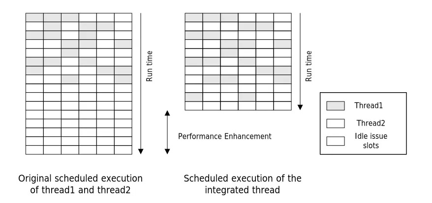
benefit of STI is that the integration of threads increases the number of independent instructions, allowing

the compiler to generate a more efficient instruction schedule and hence faster runtime performance. STI

can convert abundant thread-level-parallelism (TLP) in multimedia applications to

instruction-level-parallelism (ILP) to achieve implicit multithreading in a single-threaded machine with no architectural

support. Figure 1.1 illustrates how the integrated thread can achieve performance improvement. In this

research, we leverage this benefit for improving the performance of multimedia applications running on

VLIW/EPIC machine. We integrate parallel procedure calls, which can be seen as parallel threads, to

improve run-time performance by gathering work in an application and executing it efficiently. We rely on

the programmer to identify parallel procedures, rather than rely on compiler identification. STI fuses entire

procedures together, removing the loop-boundary constraint of loop jamming or fusion. [Ersh66] It uses

code replication and other transformation as needed to reconcile control-flow differences.

Thread1

Thread2 Idle issue slots

Original scheduled execution

of thread1 and thread2 Scheduled execution of theintegrated thread

R

un

t

im

e

R

un

t

im

e

Performance Enhancement

(10)

Whole-program (interprocedural) optimization methods extend the compiler’s scope beyond the call

boundaries defined by the programmer to potentially encompass the entire program. The methods include

interprocedural data-flow analysis, procedure inlining and procedure cloning. Procedure cloning consists of

creating multiple versions of an individual procedure based upon similar call parameters or profiling

information. Each version can then be optimized as needed, with improved data-flow analysis precision

resulting in better interprocedural analysis. The call sites are then modified to call the appropriately

optimized version of the procedure. Procedure cloning is an alternative to inlining; a single optimized clone

handles similar calls, reducing code expansion. Cooper and Hall [CHK93] [Hall91] used procedure cloning

to enable improved interprocedural constant propagation analysis in the matrix300 from SPEC 89.

Selective specialization for object-oriented languages corresponds to procedure cloning. Dean at el.

[DCG94] use static analysis and profile data to select procedures to specialize.

STI proposes a way to provide procedure clones by integrating parallel procedure calls exploiting TLP

in an application. The novelty is in providing clone procedures that do the work of two or three procedures

concurrently (“conjoined clones”) through software thread integration. This enables work to be gathered for

efficient execution by the clones. This approach is also different from other proposed architectural models

to exploit TLP in an application, as it does not require any architectural support. In this thesis, we present

the methods to clone and integrate procedures in multimedia applications to improve the run-time

performance and introduce the concept of ‘Smart RTOS’ as a model for utilizing integrated threads

efficiently in embedded systems. Then we present the results which show how much performance benefit

we can achieve using STI and what limits it with the sample application. We examine JPEG on an

ItaniumTM processor compiling it with four different compilers. (gcc, ORCC, Pro64, and Intel C++)

The organization of this thesis is as follows. Chapter 2 presents the general methodology from finding

threads for integration to performing integration and execution models for integrated threads. Chapter 3

describes how we performed the integration for JPEG application and the overview of the experiment.

Chapter 4 presents and analyzes the experimental results. The thesis ends with the conclusions in Chapter

(11)

4

2. Integration Methods and Execution Models

Planning and performing STI requires several steps. We choose the candidate procedures from the

application and examine the applicability of STI. Then we perform integration to create the integrated

versions of target procedures and use those in the application with a certain model of execution. These five

steps are presented in detail below.

2.1. Identify the candidate procedures for integration

The first stage of integration is to choose the candidate procedures for integration from the application.

Most programs are composed of many procedures, which are called and call each other. However,

programs tend to spend most of their execution time for running a few procedures. The best tool for

identifying those is profiling, which is supported by most compilers (e.g. gprof in gnu tools). It is quite

clear that improving the performance of the program is best accomplished by improving the procedure take

most of the program’s time. Profiling shows how much percentage of time is spent on each procedure in an

application. The procedure which consumes more time than any other else will be the first candidate for

integration.

For multimedia applications, those procedures usually include compute intensive code fragments, which

most DSP benchmark suites call DSP-Kernels such as filter operations (FIR/IIR), and frequency-time

transformations. (FFT, DCT) [ZMSM94] Those routines have more loop-intensive structures and handle

larger data sets, which requires more memory bandwidth then normal applications. [FWL99]

2.2. Examine parallelism in the candidate procedure

The second step is to examine parallelism in the candidate procedure because integration requires

(12)

instruction to loop and procedure levels based on the distance of the independent instructions. Instruction

level parallelism (ILP) is the execution of independent instructions within limited size of instruction

window or somewhat bigger scope. ILP architectures and compilers are designed to exploit this level of

parallelism. There is another level of parallelism called thread level parallelism (TLP), where independent

instructions are far more distant than those in ILP. This parallelism cannot be found and used easily by

ILP-centric hardware mechanisms or compilers because independent instructions are too distant to be detected

with a small instruction window. [MOAV99]

The method proposed here is a software technique to use STI for converting procedure-level parallelism

to ILP. Though there are other levels of TLP in the applications, we only focus on this type. Multimedia

applications tend to spend most of their execution time to run compute intensive routines. Those routines

handle large sets of data located in memory. They are iteratively called in the applications and the input and

output sets for each call are independent of each other. This characteristic is distinct because media

applications process their large data by separation into blocks. For example, FDCT/IDCT (forward/inverse

discrete cosine transform), one of the most common processes in image applications, handles a 8x8

independent block of pixels; these procedures are called many times in the applications like JPEG and

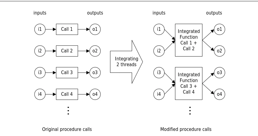
MPEG. We use this purely independent procedure-level data parallelism: 1) Each procedure call handles

its own data set, input and output. 2) Those data sets are purely independent of each other requiring no

synchronizations between calls. Our strategy for STI is to rewrite the target procedure to handle multiple

sets of data at once. An integrated procedure joins multiple independent sets of instruction streams and can

offer more ILP than the original procedure. Figure 2.1 shows the existing parallel procedure calls and

strategy for integration. Parallel procedure calls can be seen as parallel threads.

Detecting this parallelism is not an easy task; much work has been done to automatically extract

multiple threads out of a single program for execution on processors with multiple instruction streams. For

example, the PARADIGM compiler automatically extracts abundant loop level parallelism in the scientific

programs and distributes program data for distributed-memory multicomputers. [BCG+95] The

Multiscalar approach uses a compiler to extract tasks from a sequential program for concurrent speculative

(13)

6

parallelism with Program Dependence Graphs (PDG) and performs automatic partitioning and scheduling

for XIMD processors. [Newb97] Nevertheless, identifying procedure-level parallelism requires

interprocedural data flow analysis, which is still quite difficult in the general case. [Ryde82] We are not

trying to solve this problem. Instead, we assume that application developers will extract parallel threads

whether automatically or manually. We only present a method to execute the parallel procedures more

efficiently on a single instruction stream processor. In this research, we examine parallelism in a specific

procedure based on algorithmic understanding of the application and observation of the program’s

behavior.

Call 1

Call 2

Call 3

Call 4

o1 i1

i2

i3

i4

o2

o3

o4

Original procedure calls

inputs outputs

Integrating 2 threads

Integrated Function Call 1 + Call 2

Integrated Function Call 3 + Call 4

o1 i1

i2

i3

i4

o2

o3

o4

Modified procedure calls

inputs outputs

..

.

_..

.

Figure 2.1. Purely independent procedure-level parallelism and strategy for STI

2.3. Evaluate the constraints for integration

The third step is to evaluate the potential difficulties for integration. Since integration needs code

transformation in procedure level, it depends on the particular code structure rather than the general

characteristics of the application. Even though procedure calls are independent, the code structure of the

(14)

The first constraint comes from the data tractability for moving calls. To call the integrated procedure in

the application, calls must be advanced or delayed to the position where another procedure is called.

Though the procedure calls are independent, moving calls for integration causes another data flow issue:

the change of def-use chain for inputs and outputs. It requires complicated interprocedural analysis. In this

research, we limit that complexity by choosing the procedures which give a reasonable scope to examine it

manually. When the calls are too apart through many procedure calls, it is hard to track all data sets and

possible changes. It can be identified by constructing the expanded call graph, which shows the hierarchy

and behavior of the procedure call pattern, using a profiler and a debugger.

Call graph profile listing can be used to construct the call graph of the program, which shows the

hierarchy of procedure calls. [GKM82] Figure 2.2 shows the simplified call graph of DJPEG application,

which includes only candidate functions from DJPEG application. Rectangles represent procedures. Callers

and callees are connected with arrows, the number on which represents number of calls from callers to

callees. Since the call graph shows only the static behavior of procedure calls, the pattern of multiple call

instances should be also obtained with the help of a debugger like gdb. By instantiating all call instances

from the call graph, the expanded call graph is constructed as we see in Figure 2.3.

Main()

JRS()

PDCM()

SU()

YRC() DO()

JF() DM() JII() 512

1

1/16 1

32 32 192 1

JRS: jpeg_read_scanlines

PDCM: process_data_context_main DO: decompress_onepass SU: sep_updsample JF: jzero_far DM: decode_mcu JII: jpeg_idct_islow YRC: ycc_rgb_convert

(15)

8

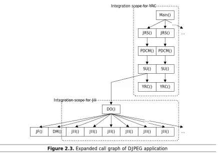
Data tractability for integrating multiple procedure calls can be examined by observing the expanded

call graph. If multiple instances of calls are activated with nested intervening calls, it is not easy to make

sure that all the inputs and outputs are not changed through those procedure calls. For example, the multiple

instances of the candidate function YRC in DJPEG (in Figure 2.3) are activated by an ancestor procedure

Main with three intervening procedure calls, JRS, PDCM and SU. When we defer the 1st YRC call to the

2nd one for parallel execution, it is hard to make sure that inputs and outputs of that procedure call are not

changed through four procedure calls. On the other hand, the multiple calls of the candidate procedure JII

are activated by a function DO, which is located just above JII. Therefore, JII gives a reasonable code scope

to track data for integration while YRC does not. (The dotted rectangles in Figure 2.3 represent the

respective scopes for two respective procedures.) Too big code scope for tracking data would require

interprocedural data flow analysis, which is considered to be too complicated. We focus only on procedures

like JII, in which calls are adjacent and activated by one parent procedure call. It gives a reasonable scope

(16)

DO()

JF() DM() JII() JII() JII() JII() JII() JII() ... Main()

JRS()

PDCM()

SU()

YRC()

JRS() ...

PDCM()

SU()

YRC() ...

... Integration scope for JII

Integration scope for YRC

Figure 2.3. Expanded call graph of DJPEG application

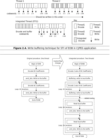
The second constraint comes from the reuse of the buffer. Some buffers need to be duplicated to allow

concurrent execution of separate procedures. Since multimedia applications use large data sets, the input

and output buffers are often reused in order to save memory space. If the buffer is composed of multiple

levels with variable sizes and forces outputs to be written in a specific order, a buffering technique need to

be be used for integration. For example, Huffman encoding, which is used for encoding DCT coefficients

in CJPEG, is a scheme in which encoded codeword has a variable bit size. The buffer to write codewords is

composed of multiple levels and the procedure, emit_bits, is in charge of writing a codeword to the buffer

sequentially in bit level. It writes codewords to another lower level of buffer when its buffer is full. The

original procedure, encode_one_block (EOB), calls that procedure, emit_bits whenever it computes a

codeword. We normally cannot interleave all the codes in that procedure because the written order also

would be interleaved by performing integration and mix up the codewords. To solve this problem, writing

(17)

10

be written to it after it finishes decoding. Figure 2.4 illustrates the way to maintain the write order and

Figure 2.5 shows how the control flow of the integrated procedure should be redesigned. Therefore,

buffering makes the written order same as the original procedure but requires an additional local buffer,

which could increase data accesses and register pressure.

On the other hand, integration is impossible if there is this kind of constraint in read side. The procedure

which performs Huffman decoding, decode_mcu (DM) in DJPEG is the counter part of EOB in CJPEG.

Decoding cannot be parallelized because the position of the buffer, from which the codewords for the next

(18)

Thread1

Encode Thread1Write

Thread2

Encode Thread2Write

1-1 1-2 1-3 1-4 1-63 1-64 2-1 2-2 2-3 2-4 2-63 2-64

Thread 1 Thread 2

codewords

Should be written in this order ...

Integrated Thread (STI2)

... ... ... Integrated Encode ... 1-1 1-2 1-3 1-64 2-1 2-2 2-3 2-64

Encode and buffer codewords

... ...

Key

Write

Figure 2.4. Write buffering technique for STI of EOB in CJPEG application

Encode DC Coefficients

Encode AC Coefficients emit_bits: Write to the buffer

emit_bits: Write to the buffer Begin of EOB

End of EOB Loop: 63 iterations

Original procedure: One thread

Encode 2 sets of DC Coefficients

Encode 2 sets of AC Coefficients Buffering: write to local buffer

Buffering: write to local buffer Begin of EOB2

Loop: 63 iterations

Integrated procedure: Two threads

Read local buffer

emit_bits: Write to the buffer

Read local buffer

emit_bits: Write to the buffer

End of EOB Loop: 64 iterations

Loop: 64 iterations Control flow

changes

Added routine

(19)

12 Code Predicate Loop Thread1 Thread2 Integrated Thread Key 1 2 3 4 P1 P2 L1 T F 1' 2' 3' 4' P1' P2 L1 T F

1+1' P1 4+4' P2 L1

T F

2+2' 2+3' 3+2' 3+3'

P1' P1'

T F T F

Thread1 Thread2 1 2 3 4 P1 P2

b. Loop with a conditional (P1 is data-dependent and P2 is not.)

Integrated thread CFG

2 1

c. Loop with different iterations (P1 is data-dependent.)

1 2 P1 L1

Thread1

P1 Thread2 L1

1' 2' P1&P1' L1 Integrated thread 1+1' 2+2' P1' CFG

1 2 P1 L1

L1

1' 2' P1'

2 1

a. Procedure with a loop (P1 is data-independent.)

1 2 3 Thread1 P1 Integrated thread 3 P1 L1 Thread2 P1 L1 P1 L1 1' 2' 3' 1+1' 2+2' 3+3' CFG P1 P1'

(20)

2.4. Performing integration

When the candidate procedure has the desired parallelism and few constraints for the code

transformations, we can determine which procedures to integrate. We can also determine how many

procedure calls can be integrated from the expanded call graph. Since we only consider integrating adjacent

calls from one parent procedure, how many threads can be integrated is limited by number of adjacent calls.

For example, integration of calls from 2 to 6 of JII is possible. However, integrating too many procedure

calls is not desirable because it increases the code size excessively.

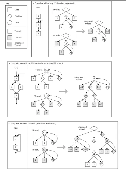
Many cases and corresponding code transform techniques for STI have been already demonstrated by

previous work. [DS98] [Dean00] [Dean02] STI uses the control dependence graph (CDG, a subset of the

program dependence graph) [FOW87] to represent the structure of the program, which simplifies analysis

and transformation. STI interleaves multiple procedures, with each implementing part of a thread. For

consistency with previous work we refer to the separate copies of the procedure to be integrated as threads.

Integration of identical threads is a simple case. Figure 2.6 demonstrates the cases and corresponding code

transformation, which can happen integrating the same threads which handle different data sets. This

transformation can be applied repeatedly and hierarchically, enabling code motion into a variety of nested

control structures. Integration of basic blocks involves fusing two blocks. (case a) To move code into a

conditional, it is replicated into each case. (case b) Code is moved into a loop with guarding or splitting.

Finally, loops are moved into other loops through combinations of loop fusion, peeling and splitting. (case

c) These transformations can be seen as a superset of loop jamming or fusion. They jam not only loops but

also all code (including loops and conditionals) from multiple procedures or threads, greatly increasing its

domain.

Code transformation can be done in two different levels: assembly or high-level-language (HLL) level.

Assembly level integration is preferred generally because it schedules instructions with fine-grain

concurrency. It especially works efficiently with processors like superscalars which have dynamic

scheduling capabilities because find-grained independent instructions are more likely to be executed

(21)

14

scheduling constraints like resource distribution into appropriate issue slots. Though HLL level integration

tends to result in coarse-grain concurrency, it can be chosen as an alternative because it can reduce a

programmer’s effort when there is no automatic tool for code transformation. Furthermore, if there is a

good compiler support for VLIW or a large instruction window size in superscalar, it could offer fine-grain

concurrency. There is no general answer for which level integration is better. It primarily depends on the

capabilities of the tools and compilers.

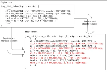
Whether the integration is done at either assembly or HLL level, it requires two steps. The first is to

duplicate and interleave the code (instructions). The second is to rename and allocate new local variables

and procedure parameters (registers) for the duplicated code. Figure 2.7 demonstrates how the integrated

procedure can be written while performing integration of two threads at the C level. The second step is

quite straightforward during HLL level integration because the compiler takes care of allocating registers.

Not all local variables (registers) are duplicated because there could be some variables shared by the

threads.

jpeg_idct_islow(inptr, outptr) { (...)

z2 = DEQUANTIZE(inptr[DCTSIZE*2], quantptr[DCTSIZE*2]); z3 = DEQUANTIZE(inptr[DCTSIZE*6], quantptr[DCTSIZE*6]); z1 = MULTIPLY(z2 + z3, FIX_0_541196100);

tmp2 = z1 + MULTIPLY(z3, - FIX_1_847759065); tmp3 = z1 + MULTIPLY(z2, FIX_0_765366865); (...)

}

jpeg_idct_islow_sti2(inptr, inptr_2, outptr, outptr_2) { (...)

z2 = DEQUANTIZE(inptr[DCTSIZE*2], quantptr[DCTSIZE*2]);

z2_2 = DEQUANTIZE(inptr_2[DCTSIZE*2], quantptr_2[DCTSIZE*2]);

z3 = DEQUANTIZE(inptr[DCTSIZE*6], quantptr[DCTSIZE*6]);

z3_2 = DEQUANTIZE(inptr_2[DCTSIZE*6], quantptr_2[DCTSIZE*6]);

z1 = MULTIPLY(z2 + z3, FIX_0_541196100);

z1_2 = MULTIPLY(z2_2 + z3_2, FIX_0_541196100);

tmp2 = z1 + MULTIPLY(z3, - FIX_1_847759065);

tmp2_2 = z1_2 + MULTIPLY(z3_2, - FIX_1_847759065);

tmp3 = z1 + MULTIPLY(z2, FIX_0_765366865);

tmp3_2 = z1_2 + MULTIPLY(z2_2, FIX_0_765366865);

(...) }

Original code

Modified code

Duplicate and interleave the code

Rename and allocate variables

(22)

There are two expected side effects from these code transforms. One is a code size increase (code

expansion), and the other is a register pressure increase. The best-case code size increase is approximately

proportional to the number of integrated threads. If there is a conditional which depends on the data, the

code size increase is exponential to the number of threads and conditional nesting depth. Code size increase

has a significant impact on performance if it exceeds a certain threshold, which determined by instruction

cache size and levels. The number of registers also increases linearly with the number of integrated

approximately. It also has a negative influence on the performance if it causes register spills due to

insufficient physical registers. Control flow does not affect the register pressure.

Negative impact on performance from both exceeds the benefit from STI if the code size is excessive.

Performance degradation from cache misses is especially significant if the code size is larger than L1

I-cache size. Optimizations, which increase the code size significantly (such as loop unrolling), should be

disabled before integration in such cases. Though code size of the integrated procedure cannot be measured

before integration, the expected code size can be estimated based on that of that of the original procedure.

If it exceeds the L1 I-cache size much, we cannot expect performance improvement by integration.

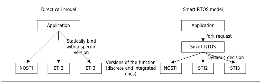
2.5. Building execution models

There are two approaches to use the integrated threads in the applications. Figure 2.8 compares these

two approaches. The first approach is to modify the application to call integrated threads directly by

replacing original procedure calls with integrated procedure calls. (Static approach: ‘direct call’) This is

appropriate for a simple system where there is only one application running and we are interested only in

improving its performance. The second is to develop a ‘Smart RTOS’ to select the efficient version of the

procedure dynamically. (Dynamic approach: ‘Smart RTOS’) This is useful for a complicated system where

(23)

16

Application Application

NOSTI STI2 STI3

Smart RTOS

NOSTI STI2 STI3

Direct call model Smart RTOS model

Versions of the function (discrete and integrated

ones)

fork request

Dynamic decision Statically bind

with a specific version

Figure 2.8. Two execution models: a ‘direct call’ and a ‘Smart RTOS’

(1) Direct call

Direct call is the simple way to use the integrated threads. After writing the integrated versions of the

target procedures, we include those in the original source code and modify the caller procedure to call the

specific version of the callee procedure every time. Figure 2.9 illustrates the simple execution models to

run integrated versions of JII procedure in the DJPEG application.

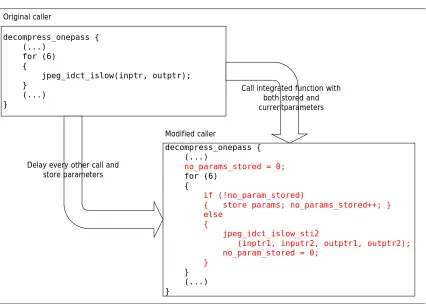
Typically the caller procedure is organized to call the target procedure a certain number of times with

the form of a loop. Since the integrated procedure handles multiple calls at once, the caller must delay the

calls and store the procedure parameters until it has data for the multiple calls. Then it calls the integrated

procedure with multiple sets of parameters. Some local variables for storing parameters for delayed calls

and for organizing the control flow are allocated to the caller and control flow becomes slightly more

complicated than before. As a result, some overhead is unavoidable from register pressure and branch

misprediction. Figure 2.10 shows how the caller was modified for integrated version of JII in DJPEG

application. Not all caller procedure are as simple as this example but some variations could be easily taken

(24)

DO()

JF() DM() _data1JII() _data2JII() _data3JII() _data4JII() _data5JII() _data6JII() ... ...

NOSTI: Original execution

DO()

JF() DM() _data1+data2JII2() _data3+data4JII2() _data5+data6JII2() ... ...

DO()

JF() DM() _{data1+data2+data3}JII3() _{data4+data5+data6}JII3() ... ...

STI2: Always calls 2-integrated thread

DO: decompress_onspass JF: jzero_far DM: decode_mcu JII: jpeg_idct_islow

JII2: jpeg_idct_islow_sti2

JII3: jpeg_idct_islow_sti3

Figure 2.9. ‘Direct call’ execution models for 3 versions of JII in DJPEG.

decompress_onepass { (...)

for (6) {

jpeg_idct_islow(inptr, outptr); }

(...) }

decompress_onepass { (...)

no_params_stored = 0;

for (6) {

if (!no_param_stored)

{ store params; no_params_stored++; } else

{

jpeg_idct_islow_sti2

(inptr1, inputr2, outptr1, outptr2); no_param_stored = 0;

}

} (...) }

Original caller

Modified caller

Delay every other call and store parameters

Call integrated function with both stored and currentparameters

(25)

18

The application can be optimized using feedback based on the performance of each version of the

procedure. We measure the performance of various versions of the application (or procedures), varying the

level of integration in the procedures. Optimization is achieved by selecting the most efficient version. This

grows more important if we have more than one procedure with various versions in the application. For

example, we have three versions – original, 2-thread integrated, 3-thread integrated – of FDCT and Encode

(Huffman encoding) in CJPEG application. From the nine possible ways to invoke those two threads, the

best combination can be obtained by choosing most efficient version of respective FDCT and Encode. This

leads to optimization of the application.

(2) Smart RTOS

A ‘Smart RTOS’ can be introduced to run the integrated threads efficiently. If we succeed in writing

multiple versions of the target procedures, we create a library of integrated and discrete versions of

procedures. We modify the program to replace the original procedure calls with RTOS thread-forking

requests. Then we enhance the RTOS to interpret thread-forking requests. It can either choose the best

version of a thread to execute from library of multiple versions and invoke it immediately or else defer its

execution, waiting for another thread request which would enable the execution of an integrated version.

The goal of the selection is to choose a version of the thread which has been integrated with one or more

other threads and is most efficient.

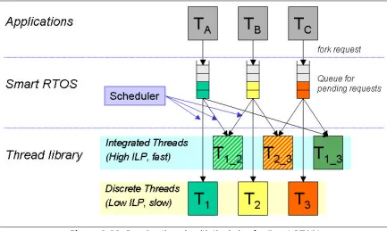
Figure 2.11 illustrates how the RTOS uses integrated threads. Thread A, B, and C in applications (a

single application or different applications or multiple instances of the same application) send

thread-forking requests to the Smart RTOS. The Smart RTOS saves those requests into their respective queues for

different threads, and the scheduler in the Smart RTOS determines whether to execute immediately or defer

execution. When it decides to execute a specific thread, it also determines which version of thread is the

most efficient to run at that moment considering combinations of all pending threads in the queues. Then it

(26)

Figure 2.11. Running threads with the help of a ‘Smart RTOS’

A Smart RTOS gives much flexibility to take advantage of STI. First, it enables exploiting the

parallelism of multiple applications. Just as a single instruction stream has an ILP limit, a single application

has limited TLP itself. In a complicated system which runs many applications, there is more TLP which can

be used for STI. For example, a cell phone base station processes data for multiple voice channels for many

users simultaneously. We can use STI technique for the computation kernels for encoding and decoding

voice and achieve performance improvements. Second, a Smart RTOS can adaptively offer optimal

executions for changing workload of a system because it is based on dynamic decisions. If requests for a

certain thread have reduced significantly at some moment, it can monitor that change and try not to wait for

that request. Instead it can try to invoke a discrete version of that thread immediately, which gives quicker

execution. Third, the goal of scheduling can be extended. Now we are focusing only on improving the

performance of applications but most embedded systems require meeting deadlines for some processes. An

RTOS can maintain the information about the execution time of various versions of the threads and invoke

(27)

20

However, there are some unavoidable consequences in this approach. First, the RTOS will introduce

some overhead for the execution depending on the complexity of the scheduler algorithm. If the algorithm

is too computationally expensive, it will exceed the benefits of integrated threads. Second, kernel

procedures of the applications should be carefully designed to share requests and applications should be

written in that way. The same procedures from different applications should have the same procedural

interface in order to share requests for that thread. As this thesis is an exploration of the potential

performance impact of integrating threads, the Smart RTOS concept is not examined further here and is left

(28)

3. Integration of JPEG Application and Overview of the

Experiment

We chose the JPEG application as an example of the multimedia workload. We performed STI for

JPEG application as presented in Chapter 2. Three target procedures were identified and integrated

manually at the C source code level and executed in the application with a ‘direct call’ execution model on

an ItaniumTM machine. The objective of the experiment is to build up the general approach to perform STI

and to examine performance benefits and bottlenecks. We do not use a ‘Smart RTOS’ model for this

experiment because we focus only on measuring and analyzing the performance of integrated threads and

utilization of the processor.

3.1. Sample application: JPEG

JPEG is a standard image compression algorithm and one of the most frequently used one in

multimedia applications. It is contained in the MediaBench benchmark suite, a popular benchmark for

representing multimedia workloads. [LPM97] Source code was obtained from Independent JPEG Group.

Every configuration setting was maintained from the original one but the input file. We used

512x512x24bit lena.ppm, which is a standard image for image compression research.

JPEG is composed of two application: DJPEG (Decompress JPEG) and CJPEG (Compress JPEG).

Understanding the algorithm of the application helps find existing parallelism in the application. The basic

(29)

22 Encoded image lena.ppm [Preoprocess] Read image Image preparation Block preparation [FDCT] Forward DCT Quatize [Encoding] Huffman/Differential Encoding [Postprocess] Frame build Write image Encoded image lena.jpg Algorithm: CJPEG Encoded image lena.jpg [Preprocess] Read image Frame decode [Decoding] Huffman/Differential Decoding [IDCT] Dequatize Inverse DCT [Postprocess] Image build Write image Decoded image lena.ppm Algorithm: DJPEG

Figure 3.1. Algorithms of CJPEG and DJPEG

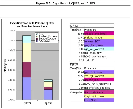
Execution tim e of CJPEG and DJPEG and function breakdow n

0.0E+00 2.0E+07 4.0E+07 6.0E+07 8.0E+07 1.0E+08 1.2E+08 1.4E+08 CJPEG DJPEG CPU Cycles Etc. Pre/Post Process Encode/Decode FDCT/IDCT

Figure 3.2. Execution time and procedure breakdown of CJPEG and DJPEG

CJPEG

Time(%) Procedure

23.86encode_one_block 20.45preload_image 18.18forward_DCT 17.05jpeg_fdct_islow 9.09rgb_ycc_convert 4.55get_24bit_row 4.55h2v2_downsample 2.27__divdi3 DJPEG

Time(%) Procedure 51.02jpeg_idct_islow 26.53ycc_rgb_convert 12.24decode_mcu

8.16h2v2_fancy_upsample 2.04decompress_onepass Categories Encode/Decode Pre/Post Process

(30)

3.2. Integration Method

Figure 3.2 shows the execution time and procedure breakdown of CPU cycles from gprof compiled by

GCC with –O2 optimization. DJPEG uses most of its execution time to perform IDCT (Inverse Discrete

Cosine Transform). CJPEG also uses significant amounts of time to perform FDCT (Forward DCT) and

Encoding (Huffman Encoding).

FDCT/IDCT is a common technique for compressing and decompressing an image. The existing

parallelism is that one procedure call performs FDCT/IDCT for an 8x8 pixel macro block; the input and

output data of every procedure call are independent. Similarly Encode/Decode processes a block of data per

procedure call and has the same level of parallelism as FDCT/IDCT has.

We perform the integration of two and three threads for IDCT, jpeg_idct_islow (JII), in DJPEG and

FDCT, forward_DCT (FD) and jpeg_fdct_islow (JFI), Encode, encode_one_block (EOB), in CJPEG.

Decode, decode_mcu (DM), in DJPEG cannot be parallelized because of the data dependencies between

buffer positions of the blocks. We do not perform the integration for other procedures, rgb_ycc_convert

(RYC) and ycc_rgb_convert (YRC) because their calls are far apart from each other through three ancestor

procedures, which would cause too many changes of the programs. (See Figure 2.3.)

Code transformation is done at the C source level using the techniques just presented. IDCT is

composed of two loops with identical control flow and a conditional which depends on the input data. The

control flow of the integrated procedure is structured to handle all possible execution paths. (case b in

Figure 2.6) The control flow of Encode in CJPEG is also similar as it has a loop with a data-dependant

predicate. The previously mentioned buffering technique is applied to maintain the write order of

codewords during integration of EOB. FDCT is composed of two procedures, FD and JFI, for which are

integrated respectively. Even though there is a nest call from FD to JFI, the control flow is quite

straightforward as it is an extension of a procedure with a loop. (case a in Figure 2.6) In this case,

(31)

24

We invoke the integrated threads by the ‘direct call’ execution model. Three different versions of caller

procedures for the respective versions are written and included in the original source code, and are

compiled to different versions of the application with conditional compile flags. Then we measure the

performance of the target procedures with those versions. Finally, we build the best-optimized version of

the application by selecting the version with the best performance.

Since this experiment is focused on the performance improvement from STI, it does not include any

detailed model for the ‘Smart RTOS’. However, ‘direct call’ execution model just represents the simplest

model of a ‘Smart RTOS’, which chooses the same version of the thread at the every thread-forking request

without any RTOS overhead. Original execution and two implemented models (STI2 and STI3) for IDCT

in DJPEG are shown in Figure 2.8. Figure 3.3 illustrates models for FDCT and EOB in CJPEG. The call

pattern of JFI is not as straightforward as JII is in DJPEG and EOB in CJPEG because the procedure FD,

which is responsible for partial function for FDCT, is located between Compress_data and JFI. The

(32)

JFI2() data1+data2

FD3() EMH()

FD: forward_DCT JFI: jpeg_fdct_islow EMH: encode_mcu_huff EOB: encode_one_block

FD2: forward_DCT_sti2() JFI2: jpeg_fdct_islow_sti2() EOB2: encode_one_block_sti2()

JFI2()

dta3+data4 data5+data6JFI2() data1+data2EOB2() data3+data4EOB2() data5+data6EOB2()

JFI3()

data1+data2+data5 data1+data2+data3EOB3() data4+data5+data6EOB3() FD3()

JFI3() data3+data4+data6

FD3: forward_DCT_sti3() JFI3: jpeg_fdct_islow_sti3() EOB3: encode_one_block_sti3() 3rd_{and 4}th_call

Compress_data()

FD() FD() FD() FD() 1st_call ₂nd_{call 3}rd_call4th_call

EMH() 1st_call

JFI()

data1 data2JFI() data3JFI() data4JFI() data5JFI() data6JFI() EOB()data1 EOB()data2 EOB()data3 EOB()data4 EOB()data5 EOB()data6

Compress_data()

FD2() FD2() FD2() 1st_call ₂nd_call

EMH() 1st_call

2nd_{and 4}th_call

Compress_data()

1st_{and 3}rd_call ₁st_call

NOSTI: Original execution

Figure 3.3. ‘Direct call’ execution models for FDCT and EOB in CJPEG application

3.3. Overview of the experiment and evaluation methods

Three versions of source code (1/ NOSTI: original discrete version, 2/ STI2: 2-thread-integrated, 3/

STI3: 3-thread-integrated) for respective target procedures (IDCT in DJPEG, FDCT and EOB in CJPEG)

are written and compiled with various compilers with different optimization options: GCC –O2, Pro64 –

O2, ORCC –O2 and –O3, Intel –O2, –O3, and –O2u0. (–O2 without loop unrolling) GCC is the compiler

(33)

26

Research Compiler evolved from Pro64 and Intel C++ compiler is a commercial compiler released by Intel

Corporation. Table 3.1 lists the compilers which we used in this experiment. The main reason for using

various compilers is that the performance of a program varies significantly with the compiler in

VLIW/EPIC architectures because scheduling decisions are made at compile time. The second is that we

try to observe the correlation between features of the compliers and the performance benefits of STI. Figure

3.4 presents the overview of the experiment.

DJPEG

Applications CJPEG

Threads IDCT_NOSTI

IDCT_STI2

IDCT_STI3

FDCT_NOSTI

FDCT_STI2

FDCT_STI3

Encode_NOSTI

Encode_STI2

Encode_STI3

Compilers and Optimizations

GCC -O2

Pro64 -O2

ORCC -O2 / -O3

Intel -O2 / -O3

/ -O2u0

Platform Linux for IA-64

Results Performance / IPC Cycle breakdown Compile

Run

Measure ItaniumTM_processor

(34)

Symbol Name Version License

GCC GNU C Compiler for IA-64 3.1 GNU, Open Source Pro64 SGI Pro64TM_Compiler _{Build 0.01.0-13} _{SGI, Open Source} ORCC Open Research Compiler Release 1.0.0 Open Source Intel Intel C++ Compiler 6.0 Intel, Commercial

Table 3.1. Compilers used in the experiment

The compiled programs are executed on an Intel ItaniumTM processor running Linux for IA-64. Intel

ItaniumTM processor is the implementation of IA-64 architecture proposed by Hewlett-Packard and Intel. It

features EPIC (Explicitly Parallel Instruction Computing), predication, and speculation. It can issue a

maximum of 6 instructions per clock cycle and has 2 integer, 2 memory, 3 branch, and 2 floating-point

functional units. Six instructions are encoded into a Bundle with stops and a template. A stop splits

dependent instructions and a template determines the dispersal from issue slots to functional units.

ItaniumTM has 3 levels of caches, 16K L1 data cache, 16K L1 instruction cache, 96K unified L2 cache, and

2048K unified L3 cache. It runs with an 800MHz CPU clock rate and 200MHz memory bus speed.

[Intel00]

All experimental data are captured during execution the help of the Performance Monitoring Unit

(PMU) in Itanium processor. The PMU features hardware counters, which enable the user to monitor a

specific set of pipeline events. The software tool and library pfmon make it easy to access the PMU simply

by adding macros or procedure calls to the original source code. [ME02] We measure the performance

(execution cycles or time), instruction per cycle (IPC), and cycle breakdown of the procedures, which

shows how execution cycles consist of inherent execution cycles and specific kinds of stalls. All data are

(35)

28

4. Experimental Results

Three kinds of data were obtained to observe the performance and execution behavior of the integrated

threads.

(1) CPU cycles, speedup by STI, and IPC

CPU cycles (or execution time) of different versions of the respective target procedures are measured

and normalized compared with the performance of the original function compiled with GCC-O2 so that it

indicates performance. Percentage speedup is plotted comparing the performance of the integrated version

with the original one. We also measure number of instructions retired and compute IPC.

(2) Cycle and speedup breakdown

Every cycle spent on running program on Itanium can be separated in two categories: The first is an

‘inherent execution cycle’, a cycle used to do the real work of the program and the other is a ‘stall’, the

cycles lost waiting for a hardware resource to become available. The stall can be also subdivided to seven

categories: Data access, dependencies, RSE activities, Issue limit, Instruction access, Branch re-steers, and

Taken branches. Table 4.1 shows how each category is related to the specific pipeline event. [Intel01]

We measure the cycle breakdown of the each procedure for identifying the benefits and bottlenecks of

STI. From those data, we also derive and plot percentage speedup breakdown showing from which

categories a performance increase or decrease occurs. By adding numbers of bars with the same color in

that chart, we find the overall speedup from STI. The categories which have positive bars contribute to

speedup, and those with negative bars cause slowdown.

(36)

STI causes code size increase. We measured the pure code size of the procedure with encoded bundle

size excluding data space.

Categories Descriptions Inh. Exe.

(Inherent execution) Cycles due to the inherent execution of the program

Inst. Acc.

(Instruction access) Instruction fetch stalls due to L1 I-cache or TLB misses

Data Acc.

(Data access) Cycles lost when instructions stall waiting for their source operands from the memory subsystem, and when memory flushes arise RSE

(RSE activities) Stalls due to register stack spills to and fills from the backing store in memory

Dep.

(Scoreboard dependencies) Cycles lost when instructions stall waiting for their source operands from non-load instructions

Issue Lim.

(Issue limit) Dispersal break due to stops, port over-subscription or asymmetries

Br. Res.

(Branch resteer) Cycles lost due to branch misperdictions, ALAT flushes, serialization flushes, failed control speculation flushes, MMU-IEU bypasses and other exceptions Taken Br.

(Taken branches) Bubbles incurred on correct taken branch predictions

(37)

30 [FDCT/CJPEG] Performance 0 0.2 0.4 0.6 0.8 1 1.2 1.4 1.6 1.8 GCC-O2 Pro64-O2 ORCC-O2 ORCC-O3 Intel-O2 Int el-O3 Int el-O2-u0 Compilers Normalized Performance

NOSTI STI2 STI3

[FDCT/CJPEG] Speedup by STI

-20% -10% 0% 10% 20% 30% 40% GCC-O2 Pro64-O2 ORCC-O2 ORCC-O3 Int el-O2 Int el-O3 Int el-O2-u0 Compilers % Speedup

NOSTI STI2 STI3

[FDCT/CJPEG] IPC Variations 0 0.5 1 1.5 2 2.5 3 3.5 4 GCC-O2 Pro64-O2 ORCC-O2 ORCC-O3 Int el-O2 Int el-O3 Int el-O2-u0 Compilers

Instructions / Cycle

NOSTI STI2 STI3

[FDCT/CJPEG] Code Size 0 10000 20000 30000 40000 50000 60000 70000 GCC-O2 Pro64-O2 OR CC-O2 OR CC-O3 Int el-O2 Int el-O3 Int el-O2-u0 Compilers Bytes

NOSTI STI2 STI3

I-cache: 16K

(38)

[FDCT/CJPEG] CPU Cycle Breakdown

0.E+00 5.E+06 1.E+07 2.E+07 2.E+07 3.E+07 3.E+07

Cycles

TakenBr Br.Res. IssueLim. Dep. RSE DataAcc Inst.Acc Inh.Exe

GCC-O2 Pro64-O2 ORCC-O2 ORCC-O3 Int el-O2 Int el-O3 Int

el-O2-u0

[FDCT/CJPEG] Speedup Breakdown

-40% -30% -20% -10% 0% 10% 20% 30% 40%

Inh.Exe Inst.Acc DataAcc RSE Dep. IssueLim. Br.Res. TakenBr

Cycle Category

% Speedup

GCC-O2 STI2 GCC-O2 STI3 Pro64-O2 STI2 Pro64-O2 STI3 ORCC-O2 STI2 ORCC-O2 STI3 ORCC-O3 STI2 ORCC-O3 STI3 Int el-O2 STI2 Intel-O2 STI3 Int el-O3 STI2 Intel-O3 STI3 Int el-O2-u0 STI2 Intel-O2-u0 STI3

(39)

32 [EOB/CJPEG] Performance 0 0.2 0.4 0.6 0.8 1 1.2 1.4 1.6 1.8 GCC-O2 Pro64-O2 ORCC-O2 ORCC-O3

Int el-O2 Int el-O3

Compilers

Normalized Performance

NOSTI STI2 STI3

[EOB/CJPEG] Speedup by STI

0% 2% 4% 6% 8% 10% 12% 14% 16% 18% 20% GCC-O2 Pro64-O2 ORCC-O2 ORCC-O3

Int el-O2 Int el-O3

Compilers

% Speedup

NOSTI STI2 STI3

[EOB/CJPEG] IPC Variations 0 0.5 1 1.5 2 2.5 GCC-O2 Pro64-O2 ORCC-O2 ORCC-O3

Int el-O2 Intel-O3

Compilers

NOSTI STI2 STI3

[EOB/CJPEG] Code size 0 2000 4000 6000 8000 10000 12000 14000 16000 GCC-O2 Pro64-O2 ORCC-O2 ORCC-O3

Int el-O2 Intel-O3

Compilers

Bytes

NOSTI STI2 STI3 I-cache:16K

(40)

[EOB/CJPEG] CPU Cycle Breakdown

0.E+00 2.E+06 4.E+06 6.E+06 8.E+06 1.E+07 1.E+07 1.E+07 2.E+07

Cycles

GCC-O2 Pro64-O2 ORCC-O2 ORCC-O3 Int el-O2 Int el-O3

[EOB/CJPEG] Speedup Breakdown

-40% -30% -20% -10% 0% 10% 20% 30% 40%

Cycle Category

% Speedup

GCC-O2 STI2 GCC-O2 STI3 Pro64-O2 STI2 Pro64-O2 STI3 ORCC-O2 STI2 ORCC-O2 STI3 ORCC-O3 STI2 ORCC-O3 STI3 Intel-O2 STI2 Intel-O2 STI3 Intel-O3 STI2 Intel-O3 STI3

(41)

34 [IDCT/DJPEG] Performance 0 0.5 1 1.5 2 2.5 3 GCC-O2 Pro64-O2 ORCC-O2 ORCC-O3 Intel-O2 Intel-O3 Intel-O2-u0 Compilers Normalized Performance

NOSTI STI2 STI3

[IDCT/DJPEG] Speedup by STI

-200% -150% -100% -50% 0% 50% 100% GCC-O2 Pro64-O2 OR CC-O2 OR CC-O3 Intel-O2 Int el-O3 Int el-O2-u0 Compilers % Speedup

NOSTI STI2 STI3

[IDCT/DJPEG] IPC Variations 0 0.5 1 1.5 2 2.5 3 3.5 GCC-O2 Pro64-O2 ORCC-O2 ORCC-O3 Int el-O2 Intel-O3 Intel-O2-u0 Compilers

NOSTI STI2 STI3

[IDCT/DJPEG] Code size 0 10000 20000 30000 40000 50000 60000 70000 80000 90000 100000 GCC-O2 Pro64-O2 OR CC-O2 OR CC-O3 Int el-O2 Int el-O3 Int el-O2-u0 Compilers Bytes

NOSTI STI2 STI3

I-cache:16K

(42)

[IDCT/DJPEG] CPU Cycle Breakdown

0.E+00 5.E+06 1.E+07 2.E+07 2.E+07 3.E+07

Cycles

GCC-O2 Pro64-O2 ORCC-O2 ORCC-O3 Int el-O2 Int el-O3

Intel-O2-u0

[IDCT/DJPEG] Speedup Breakdown

-40% -30% -20% -10% 0% 10% 20% 30% 40%

Cycle Category

%Speedup

GCC-O2 STI2 GCC-O2 STI3

Pro64-O2 STI2 Pro64-O2 STI3

ORCC-O2 STI2 ORCC-O2 STI3

ORCC-O3 STI2 ORCC-O3 STI3

Int el-O2 STI2 Int el-O3 STI2

Int el-O2-u0 STI2 Int el-O2-u0 STI3

(43)

36 [App/CJPEG] Performance 0 0.2 0.4 0.6 0.8 1 1.2 1.4 1.6 1.8 GCC-O2 Pro64-O2 ORCC-O2 ORCC-O3 Int el-O2 Int el-O3 Int el-O2-u0 Compilers Normalized Performance

NOSTI STI2 STI3 B estCombo

[App/CJPEG] Speedup -5% 0% 5% 10% 15% 20% 25% 30% GCC-O2 Pro64-O2 OR CC-O2 OR CC-O3 Int el-O2 Int el-O3 Int el-O2-u0 Compilers % Speedup

NOSTI STI2 STI3 B estCombo

Figure 4.7. Performance and speedup by STI of CJPEG application

[App/DJPEG] Performance 0 0.2 0.4 0.6 0.8 1 1.2 1.4 1.6 GCC-O2 Pro64-O2 ORCC-O2 ORCC-O3 Int el-O2 Int el-O3 Int el-O2-u0 Compilers Normalized Performance

NOSTI STI2 STI3

[App/DJPEG] Speedup -60% -50% -40% -30% -20% -10% 0% 10% 20% 30% GCC-O2 Pro64-O2 OR CC-O2 OR CC-O3 Intel-O2 Int el-O3 Int el-O2-u0 Compilers % Speedup

NOSTI STI2 STI3

(44)

4.1. Integrated thread 1: FDCT in CJPEG

Figure 4.1 gives the performance, speedup by STI, IPC variations and code size of 3 versions (NOSTI,

STI2, STI3) of FDCT procedure in CJPEG application. Performance varies by compilers because they

generate different instruction streams for respective optimization strategies. The original procedure shows

the best performance with the compiler Intel-O2-u0. In all cases but Intel-O3, the performance of integrated

versions exceed that of the original versions; By integrating 2 threads, it achieves from –4.56% to +17.37%

speedup and from –11.97% to +37.49% by integrating 3 threads. 2-integrated version (STI2) compiled with

Intel-O2-u0 shows the best performance from all variations, achieving 17.37% speedup from the original

version (NOSTI).

STI increases code size; here we see code size increase between 74.63% and 100.68% by STI2 and

between 162.90% and 254.55% by STI3. Intel-O2 and Intel-O3 perform loop unrolling and generated codes

by those result in the code size much bigger than L1 I-cache size. Intel-O2-u0, which performs the same

optimization as -O2 but disabling loop unrolling, generate smaller code and achieves better performance

than other compilers. Comparing the speedup and code size, we can see code size is closely related with the

performance. When the size of the code is much bigger than the L1 I-cache (Intel-O2 and Intel-O3),

performance is degraded after integration. IPC is not closely correlated with the performance because

number of instructions generated by compilers varies much by compilers. IPC cannot be accepted as a

measure of processor utilization in this case.

Figure 4.2 shows the CPU cycle breakdown and speedup breakdown of FDCT in CJPEG application.

The composition of categories is different by compilers because each compiler has its own optimization

strategy. However, observing the changes occurring after integration gives basic information about why

and how integration achieves speedup. The second bar chart in Figure 4.2 shows the sources of speedup

(bars above the centerline) and slowdown (below it). Most of speedup results from reducing issue-limited

cycles, showing how the compilers are able to generate better schedules when given more independent

instructions. Some improvement comes from reducing data cache misses as well. Major sources of

(45)

38

integration increases code size and number of branches. Stalling on instruction access is the most

significant factor in Intel-O2 and Intel-O3 because the code size is much bigger than the I-cache size. In

such cases, integration results in performance degradation.

4.2. Integrated thread 2: EOB in CJPEG

STI2, STI3) of EOB procedure in CJPEG application. The original procedure shows the best performance

with Intel-O3. Performance of the integrated versions always exceeds that of the original ones and STI2 is

better than STI3 but Intel-O3 case; It achieves 7.38% ~ 17.38% speedup by STI2, 0.69% ~ 13.61% by

STI3. 3-integrated version (STI2) of EOB compiled with Intel-O3 shows the best performance from all

variations, achieving 13.61% speedup from the original version (NOSTI).

Code size excessively increases after the integration; it varies between 80.00% ~140.68% by STI2 and

251.43% ~ 491.53% by STI3. However, it is always smaller than I-cache size, which is different from

FDCT cases. IPC tends to increase but is not strongly correlated with the performance.

Figure 4.4 shows the CPU cycle breakdown and speedup cycle breakdown of EOB in CJPEG

application. The main source of speedup is reducing stalls from issue limit and data access. Stalls from

instruction access, dependencies and taken branch tend to increase after integration. However, stalls from

instruction access remains small portion of the total execution cycles compared with those of FDCT

because the code size always remains smaller than L1 I-cache size.

4.3. Integrated thread 3: IDCT in DJPEG

STI2, STI3) of IDCT procedure in DJPEG application. Unlike the FDCT and EOB cases, integrated

(46)

varies between -89.85% and 8.35% by STI2 and between -617.89% and 43.40% by STI3. STI3 by

Intel-O3, which shows the highest performance improvement, is considered an anomaly because the compiler

might fail to apply all possible optimizations due to too big code size. Though ORCC does the best job

compiling the original version, it does a poor job compiling the integrated versions. The performance of the

integrated versions compiled by Intel compiler also suffers except when loop unrolling is disabled.

Intel-O2-u0 achieves 3.94% speedup by STI2.

Due to the large code size of the original procedure and the large data-dependent code block in IDCT,

code size increase is significantly higher than the previous cases; It is 222.37% ~ 554.60% by STI2 and

14.13% ~ 1644.24% by STI3, which leads to the size much bigger than I-cache size. Every single case but

Intel-O3 where the code size exceeds L1 I-cache size results in performance degradation. It indicates that

STI is not always useful for improving the performance. If the code size of the original procedure is large

and code size expansion rate is high, it limits the general use of integration. However, the Intel-O2-u0 case,

where the original version shows the best performance except ORCC cases, shows 3.94% speedup by

integrating 2 threads. This shows that we can take advantage of integration by controlling optimizations in

some cases. Disabling loop unrolling result in significant performance improvement of original and

integrated versions in this case by reducing the instruction cache misses.

The cycle breakdown in Figure 4.6 shows that the portion of the stalls from instruction access is a

significant factor in the cases where the code size is much bigger than L1 I-cache size. The speedup

breakdown presents that integrated versions compiled by ORCC increases most kinds of stalls. Other than

ORCC cases, integration tends to decrease inherent execution cycles and stalls from data access,

dependencies, and issue limits. Though there are some sources for speedup, slowdown by increase of

instruction cache misses is too crucial so that it fails to achieve speedup by STI in most cases.

4.4. Overall Performance Benefit

These results show how integration helps the performance of parallel threads in JPEG application.

(47)

40

DJPEG does not. Since integrated versions of two procedures in CJPEG show a significant speedup, we

can optimize CJPEG application by invoking the most efficient thread. NOSTI in Figure 4.7 represents

execution of the original version for both EOB and FDCT, and STI2 shows the 2-thread-integrated version

for both and vice versa. There are nine combinations of choosing 3 versions of threads for both EOB and

FDCT. We also build ‘BestCombo’ by choosing the best combination for respective compilers based on the

performance results of the respective procedures and measure the performance. Table 4.2 shows how the

best combinations are chosen for respective compilers.

Figure 4.7 shows performance and speedup by STI of CJPEG application. BestCombo for GCC-O2 has

a little noise in data, which is supposed to be the caller side overhead not included in measurement of the

performance of the respective procedures. Except that case, performance improvement by choosing the best

combination is significant. Maximum speedup of CJPEG by choosing the best combination for respective

compilers varies from 0.45% to 23.78%. Intel-O2-u0 shows the best performance for original version and

BestCombo, which achieves 10.88% speedup by STI.

Figure 4.8 presents performance and speedup by STI of DJPEG application. Integrated versions

compiled by ORCC and Intel shows slowdown because integration fails to improve the performance of

IDCT. Intel-O2-u0 case shows the best performance of original version and 2-integrated version achieves

the best performance from all variations, improving 3.54% performance by STI.

Compiler Best FDCT Best EOB BestCombo

GCC –O2 STI3 STI2 FDCT_STI3 + EOB_STI2 Pro64 –O2 STI3 STI2 FDCT_STI3 + EOB_STI2 ORCC –O2 STI3 STI2 FDCT_STI3 + EOB_STI2 ORCC –O3 STI3 STI2 FDCT_STI3 + EOB_STI2 Intel –O2 STI2 STI2 FDCT_STI2 + EOB_STI2 Intel –O3 NOSTI STI3 FDCT_NOSTI + EOB_STI2 Intel –O2u0 STI2 STI2 FDCT_STI2 + EOB_STI2

Table 4.2. Best Combination to invoke threads in CJPEG application