SPC binomial Q-charts for short or long runs

(1)

SPC Binomial Q-Charts for Short or long Runs

CHARLES P. QUESENBERRY

North Carolina State University, Raleigh, North Carolina 27695-8203

Approximately normalized control charts, called Q-Charts, are proposed· for charting a binomial random variable. Transformations are given for the two cases when the parameter p isknown before charting is begun and when itisnot known before charting is begun. These charts permit real-time charting essentially from the beginning of sampling and are especially useful for the case when p is not known in advance. These charts are all plotted in a standard normal scale and permit a flexible charts management program. For the case when p is assumed known, we present tables to compare the closeness of the control probabilities for these Q-Charts with those of the approximating normal distribution, and with those achieved by either classical 3-sigma p-Charts or with charts based on a standardized arcsin transformation chart. These results show that Q-eharts give betterappr~ximationsthan the classical p charts to the nominal normal probabilities, and -are comparable- with, but differ from, the arcsin charts.

r -I

-Introduction

In a recent paper Quese~b~~ry(1989), Q89, proposed using standardized SPC charts, called Q-charts, to control a process mean or variance for a normally distributed quality variable. Formulas were given for computing the Q-statistics for the classical case wh,en the parameters are known. and for . the case when the process parameters, Le., mean and variance, are not known, but it is desired to plot

X

and S-charts in real time from the start-up point of the operating process, especially for short runs. In the present paper we propose using a similar approach to charting for attributes, and give the required formulas for charts for a binomial parameter p.

(2)

For the case when the binomial parameter p is known, the chart proposed here would replace

the standardized p-chart, which was recently discussed in JQT by Nelson (1989) and has been

discussed in many books including Duncan (1974) and Montgomery (1985). The standardization

transformation is a linear transformation and the accuracy of the standard normal distribution

approximation to assess the probabilities associated with a chart based on it depends only upon the

well-known normal approximation for a binomial distribution. However, control charts are usually

made for situations where p is small ( perhaps p= 0.01, 0.05, 0.10, ) and for these cases the

binomial distribution is skewed and a normal distribution does not give accurate approximations,

especially in the tails of the distribution, which are important for control chart applications. In order

to achieve better approximations by the normal distribution we must consider nonlinear

transformations. In this work we introduce such a nonlinear transformation that gives improved

normal approximations for this case when the parameter p is known, and has in addition the

advantage that it permits a natural way to generalize to the case when p is unknown by the use of an

estimating function with efficient statistical inference properties. We give tables to compare the chart

based on this new transformation ·with the standardized p chart, and with another chart based on

(3)

TABLE 1: Notation for Probability and Distribution Functions Normal:

The standard normal distribution function.

The inverse of the standard normal distribution function. Binomial:

b(x; n, p)

(~)px(1

- p)n-x, X = 0,1,2, ..., n

0, elsewhere B(x; n, p) 0, x

<

0

= 1, x 2: n

[xl

=

L:

b(x'; n, p), 0

<

x

<

n x'=O

Hypergeometric:

:$ x

<

h_u

=

0, x < h_L

1, x

>

h

_u

Exact ChartstoControl a Binomial Parameter p

To prepare the way for the introduction of attributes Q-charts, we consider first the basic nature of Shewhart control charts for attributes. We illustrate the ideas with binomial distributions.

(4)

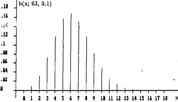
fallout) and we consider samples of size n

=

63. Then Figure 1a shows a bar-chart of the binomial distribution of nonconformities in one sample. To make a Shewhart control chart for the number of defects in each sample, we must select a lower control limit, LCL, a centerline, CL, and an upper control limit, UCL. For X the number of nonconformities in a sample, if P(X <LCL) = aL and P(X > UCL) = au, we call these limits (aL' au) probability limits. The usual 3-sigma formulas give here:

UCL = npo

+

3~npo(l-Po) = 6.3

+

3~(63)(.1)(.9) = 13.44 CL = 6.3

LCL = npo - 3~nPo(1-Po) = 6.3 - 3~(63)(.1)(.9) = - 0.84

So, for this example the 3-sigma formulas give no lower control limit and an upper control limit of UCL = 13.44. By using an algorithm for the binomial distribution function, see column 3 of Table 2, we find

P(X > UCL= 13.44) = 1 - B(13; 63, 0.1) = 1 - 0.99671 = 0.00329 However, P(X > 14)

=

1 - 0.99885

=

0.00115.

1/304

Therefore, if we wish to make a chart with the probability of exceeding UCL as close as possible to, but less than, the value for a 3-sigma normal chart, we should take UCL = 14. Note also that, in general, for a binomial chart the smallest possible integer-valued lower control limit is LCL = 1, and the probability of a point below it is

(1)

Thus, if we wish to determine the smallest value of n

sO

that the probability below LCL is less than or equal to a value aL' then we must take

In(ad

n > :-ln~(l""'--=p"""") (2) For a process with fallout of p

=

0.1, we must taken> In(0.00135)/ln(0.9)

=

62.7, in order to have the normal 3-sigma value of 0.00135 below LCL = 1. A value of n = 63 will suffice.

(5)

emphasize, that when a computer algorithm to evaluate the binomial distribution function B(x; n, p) is available, it can be used in the manner illustrated above to design a chart with exactly known probability limits (aV aU)' This is, we think, the best possible way to design a chart for the case when p is known and n is constant.

The Binomial Q-Chart for p Known

We consider next transforming observations from binomial distributions to values that can be plotted on standardized normal Q-charts. Let Xi denote an observation on a binomial random variable from a sample of size ni' Then transform the observed values to Q-statistics as in equations (3).

(3)

These values Ql' Q'2' ... can be plotted on a Q-chart with control limits at UCL

=

3, CL

=

0, and LCL = -3. More generally, a chart with approximate (aL' au) probability limits can be made by putting LCL

=

-z ,CL

=

°

and UCL

=

z . We will give some numerical results below that reflect

aL au

the accuracy of the normal approximation for the case with' 3-sigma limits, and permit the comparison of the performance of these charts with other competing charts.

To study the nature of this transformation, we consider again the binomial b(x; 63, 0.1) distribution. The b(x; 63, 0.1) probability function is shown in Figure la, and the transformed Q-binomial distribution is shown in Figure lb. This Q-distribution is, of course, a discrete distribution.

(6)

Figure 1a: The Binomial b(x; 63, 0.1) Probability Functio-!1 .18

~

b(xj 63, 0.1)

.1'

~

8 1 2 3 4 5 , 7 8 , 18 11 12 13 14 15 l' 17 18 x

.

-I

I

.

I I .12 .1 .US .Q£

.IM

.92 8

Figure 1b: The Q-Binomial Qb( qj n, p) Probability Function .18 Qb( qj n, p)

.1£ .14 .12 .1 .US .Q£

.IM

.92

a

q TABLE 2

x b(xj63,O.1) B(x;63,0.1) Q

0 .00131 .00131 -3.01

1 .00917 .01048 -2.31

2 .03159 .04207 -1.73

3 .07136 .11343 -1.21

4 .11894 .23236 -.73

5 .15594 .38830 -.28

6 .16749 .55579 .14

7 .15154 .70732 .55

8 .11786 .82519 .94

9 .08003 .90522 1.31

10 .04802 .95323 1.68

11 .02571 .97894 2.03

12 .01238 .99132 2.38

13 .00540 .99671 2.72

14 .00214 .99885 3.05

15 .00078 .99963 3.38

16 .00026 .99989 3.72

17 .00008 .99997 4.01

18 .00002 .99999 4.32

19 .00001 1.00000 4.63

(7)

When these Q-statistics are plotted on an (aL' au) control chart, it will be possible for a point to fall below the LCL only if equation (2) is satisfied. Table 2 shows the distribution of the Q-binomial distribution for n= 63 and p= 0.1. We shall denote this distribution in general by Qb(qj n, p). Note that for each value of x in the first column of Table 2, the value in the second column of the table is the binomial probability of this x, and this probability is assigned to the value of Q given in column 4, by the Q-binomial distribution Qb(qj n, p).

Example 1: To illustrate the use of the binomial Q-chart for the case when the parameter p is known, we have drawn 30 samples from a b(xj 63, 0.1) distribution and then 30 more samples from a b(xj 63, 0.15) distribution. The data are given in Table 3. The first row gives the observation number i, the second row the actual observed value x of the binomial random variable, the third the value of the statistic Q_i computed from formulas (3), and the fourth row gives the value of the Q-statistic for the case when the parameter p is not known, and will be explained below. The Q-chart for these data is shown in Figure 2a. We have drawn lines at ± 1, ± 2, ± 3. For LCL

=

-3 and UeL

=

3, we see from Table 2 above that these are actually (0.00131, 0.00329) probability limits.

Figure 2a: Binomial Q-Chart for Example 1

Q-Cha~t Co~ a known hinoMial pa~aMete~p

4

UCL 3

2

~

CL 9

-.1

-2

LCL -3

-4

(8)

TABLE 3

Data for Examples 1 and 2

i: . 1 2 3 4 5 6 7 8 9 10 11

x: 10 4 3 6 8 5 5 6 8 10 10

Qi: 1.68 -.73 -1.21 .14 .94 -.28 -.28 .14 .94 1.68 1.68

Q"_i' - -1.42 -1.18 .41 1.08 -.19 -.12 .33 1.08 1.68 1.52

I: 12 13 14 15 16 17 18 19 20 21 22

x: 5 6 5 5 9 5 6 10 5 9 5

Qi: -.28 .14 -.28 -.28 1.31 -.28 .14 1.68 -.28 1.31 -.28

Q~'l ' -.46 0 -.39 -.34 1.23 -.37 .08 1.57 -.40 1.18 -.42

I: 23 24 25 26 27 28 29 30 31 32 33

x: 3 6 5 4 6 4 6 6 8 8 11

Qi: -1.21 .14 -.28 -.73 .14 -.73 .14 .14 .94 .94 2.03

Q!'l ' -1.29 .09 -.32 -.74 .16 -.70 .19 .20 .98 .96 2.01

I: 34 35 36 37 38 39 40 41 42 43 44

x: 13 6 5 9 12 13 11 10 11 12 8

Qi: 2.72 .14 -.28 1.31 2.38 2.72 2.03 1.68 2.03 2.38 .94

Q"_i' 2.61 .01 -.40 1.18 2.2 2.46 1.73 1.34 1.65 1.95 .51

i: 45 46 47 48 49 50 51 52 53 54 55

x: 15 10 8 10 8 7 9 7 11 11 9

Qi: 3.38 1.68 .94 1.68 .94 .55 1.31 .55 2.03 2.03 1.31

Q!'_{l '} 2.86 1.15 .41 1.12 .39 .01 .75 0 1.44 1.42 .70

i: 56 57 58 59 60

x: 14 6 10 7 7

Qi: 3.05 .14 1.68 .55 .55

Q!'_{l '} 2.36 -.48 1. 01 -.09 -.09

The probabilities associated with the zones defined by the

±

1,

±

2,

±

3 standard deviation lines can be approximated by the standard normal probabilities. The goodness of the approximation depends upon both nand p and generally improves as np increases. Here np

=

(63) (0.1)

=

6.3, and the approximation may be considered marginally adequate. When the approximation is good enough, special tests for point patterns, such as some of those of Nelson (1984) can be applied to these Q-charts. We will give some results below that are helpful in judging the adequacy of the approximation. 0

(9)

The Binomial Q-Chart for p Unknown

Some further notation is needed to treat the present case. Again, we consider a sequence of values (ni' xi) for i

=

1, 2, "', and when the ith value is obtained we plot a point on the Q-chart. Let

(4)

Then we compute the Q-statistics by the equations (5).

(5)

(10)

From these properties it follows that when the process is in control, that is, when Xl' X2' ... are independent binomial random variables with constant parameter p, the Qi's are approximately independent with discrete Q distributions. Therefore the values Q2' Q3' ... can be plotted on a Q-chart. The interpretation of this chart is similar to the interpretation of the chart for p known, but certain special considerations must be observed. We will see in examples below that for the same binomial data from an in-control process the pattern of points on a chart is very similar when the Q's are computed from the formulas of (5) and when they are computed from (3), using the correct value of the parameter p. Note that the equations (5) essentially solve the problem of charting short runs of

binomial observations, since they do not require knowledge of the binomial parameter.

Note that this chart permits plotting from the second binomial sample on, but no point is plotted for the first sample. This is because the parameter p must be "estimated" from the present data sequence. Of course, from the above remarks it is seen that we do not actually make and use an estimate of p itself. The situation is similar to that in Quesenberry (1989) which gives Q-charts for normal distribution processes with unknown parameters.

(11)

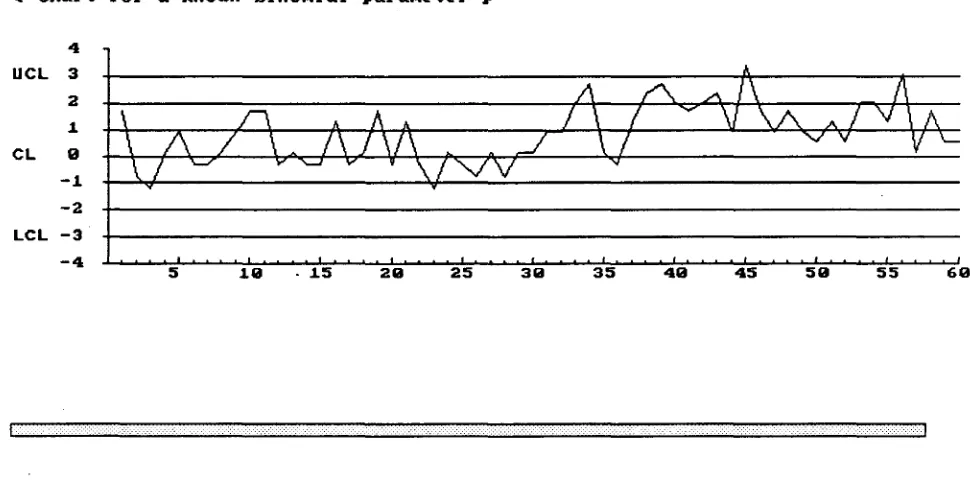
Figure 2b: Binomial Q-Chart for Example 2

Q-Chapt top Qnknown binoMial papaMetep p

4

UCL 3

2

.1

CL 9

-1.

-2

LCL -3

-4

5 1.9 .15 29 25 39 35 49 45 59 55 69

It is important to note that the Q-chart using the statistics computed in equations (3) and (5) can be made in real time, that is, when each binomial observation Xi is observed a point for it can be plotted immediately. For the equations of (5), a point is plotted for each sample, beginning with the second. This strategy is ideal for detecting changes of p at the earliest possible time.

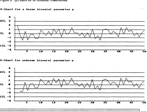
Figure 3: Q-Charts for 50 Binomial Observations

4

UCL 3

2

.1

CL 9

-1.

-2

LCL -3

-4

5 1.9 1.5 29 25 39 35 49 45 59

Q-Chapt top Qnknown binoMial papaMetep p

4

UCL 3

2

.1

CL 9

-1.

-2

LCL -3

-4

5 .19 .15 29 25 39 35 49 45 59

(12)

Example 3: To further demonstrate the similarity of the Q-charts when the parameter is not known to when it is known, we have generated 50 samples from a b(x;100,0.1). Charts for the two cases are shown in Figure 3. Note the similarity of the patterns of the two charts!

The Normal Approximation and Comparisons with Other Charts

o

We have presented formulas that can be used to transform binomial observations to values that are approximately standard normal random variables and can therefore be plotted on standard normal Shewhart type control charts. For the case when p is known, the Q-chart would in most applications today be used in place of a classical 3-sigma p, np or standardized p chart. Therefore, for this case, it would be useful to study the accuracy of the normal approximation for these Q-charts, and compare this approximation with the normal approximation for these classical charts. The classical chart that is comparable with the Q-chart is the standardized np or p chart. For x the binomial random variable with probability function b(x; n, p), this standardized statistic is given by

z

=

x - np

• ~np(1 - p) (6)

This standardization transformation, that is, subtracting the mean of x and dividing by its standard deviation, do not give a random variable z that is more normal than x. This, or any, linear transformation of a random variable change only the location and spread of the distribution, and do not affect its shape. This standardization transformation has been discussed in the statistics and quality literature by many writers. See, for example Duncan (1986) and Nelson (1989) for recent discussions in the quality literature. In order to transform the binomial random variable x to a new random variable that has a more normal distribution it is necessary to make a nonlinear transformation of x. The Q-statistic of (3) is such a nonlinear transformation.

(13)

variable have been considered in the statistical literature. In order to compare the Q-charts proposed here with what we think is about the best alternative potential method, we consider here a transformation given in Johnson and Kotz (1970), and recently presented in the quality literature by Ryan (1989). This is called an arcsin transformation and is defined by

(7)

where sin-1 is the inverse sign function. When x is a b(x; n, p) random variable y is approximately a N(O, 1) random variable.

We now give some results for comparison of charts based on the statistics z, Q and y. Suppose that we plot these statistics on control charts with lines drawn at 0, ± 1, ± 2, and ± 3. Then we partition the vertical axis into cells in terms of Q as follows:

Cell 1 is all values for Cell 2 is all values for Cell 3 is all values for Cell 4 is all values for Cell 5 is all values for Cell 6 is all values for Cell 7 is all values for Cell 8 is all values for

Q < -3

-3 $ Q

<

-2 -2

<

Q

<

-1 -1

<

Q $ 0

o

<

Q $ 1 1

<

Q $ 2

2 < Q $ 3

3 < Q

(14)

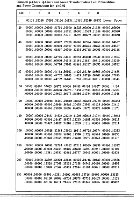
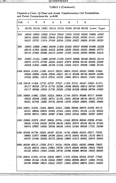
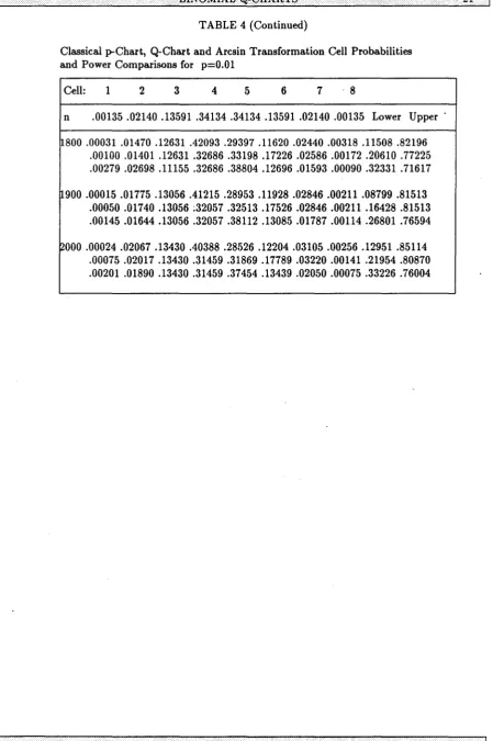
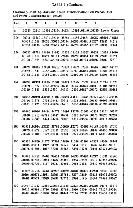
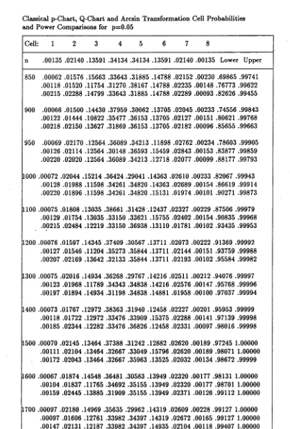
The values in the last two columns labeled "Lower" and "Upper" are probabilities of detecting certain shifts in the parameter values. The value in the "Lower" column is the probability for these values of n and p that a shift from p to p/2 will be detected by having the statistic fall below the -3 control limit, that is, fall in cell 1. The value in the "Upper" column is the probability that for these values of nand p that a shift from p to 2p will be detected by having the statistic plot above the +3 control limit, that is, fall in cell 8.

To illustrate reading these tables, consider the value in Table 4 for n

=

700. Then np

=

(700)(0.01)

=

7. The first row shows that the probability in cell 1 of a standard p-chart is zero, and that, of course, the probability of detecting a shift of p

=

0.01 to p/2

=

0.01/2

=

0.005 is also zero. The probability of a point on a standard p-chart plotting above the upper control limit when p has not changed, that is, the probability of a false alarm, is 0.00547, which is about four times the nominal normal rate of 0.00135. For the Q-chart for this case the nominal in-control cell probabilities are 0.00088 and 0.00228 for celi 1 and cell 8, respectively, and the probabilities of detecting shifts are 0.02993 and 0.32963 from the last two columns. For the arcsin y-chart the nominal in-control cell probabilities are 0.00088 and 0.00089, respectively, and the probabilities of detecting shifts are 0.02993 and 0.24232.

(15)

We have given these charts only for the three small values of p

=

0.01, 0.05 and 0.10 because the applications of these charts typically are for small values of p. Although we have computed these probabilities for eight cells, we are especially interested in the probabilities in cells 1 and 8, which are the probabilities beyond the lower and upper 3-sigma control limits. Comparison of the probabilities in some of the other cells with the normal probabilities at the top of the table allows some assessment of the accuracy of special runs tests, such as those of Nelson (1984). We make a few general comparative conclusions from these results. We think that these results show that the classical p-chart is clearly inferior to both of the other charts. Itrequires much larger sample sizes to achieve any power to detect decreases in p, and cell probabilities always differ by as much, and usually by more, from the nominal normal values than for the other charts. In particular, for all of the results in these tables the Q-chart probabilities for cells 1 and 8 are either the same as for the p-chart or - most often - they are between 0.00135 and the value for the p-chart. For cell 1 the p-chart values are too small and for cell 8 they are too large.

It is more difficult to summarize the comparison of the Q-charts and arcsin charts (based on y). Neither can be said to be a better overall approximation, but we venture a few summary remarks. The Q-chart tends to have values in cell 8 closer to, but somewhat larger than, the nominal value of 0.00135 than the y-chart, which tends to give values that are often considerably less than 0.00135, and therefore the y-chart gives less protection to detect increases in p. On the other hand, the Q-chart tends to give values in cell 1 that are smaller than 0.00135 while the y-chart tends to give values for this cell closer to but frequently larger than 0.00135. Thus the y-chart will be more sensitive to detect decreases in p, while making more false alarms. Due to this trend the y-chart gives positive probability in cell 1, and therefore some power to detect decreases of p at smaller sample sizes, for the values of p considered here.

These tables are only for charts for p known. The Q-chart for unknown p converges rapidly to

···1

(16)

the chart for known p and its limiting behavior will be the same as that for the Q-chart with known p. Due to the excellent theoretical properties of the UMVU estimator B(x) of B(x; n, p) discussed above, we think it is unlikely that one can make other charts for the unknown p case that would perform as well as the Q-chart proposed here. We close by summarizing some of the properties of the Q-charts proposed here for the consideration of potential users.

Some Properties of Binomial Q-charts:

1. These charts can be made in real time beginning with either the first binomial observation (when p is known) or the second (when p is unknown). This is especially useful for short runs or start-up processes when p is not known, since there are no established methods available today for this situation.

2. The samples do not have to be of constant size.

3. Since these charts are plotted on standard normal scale, the training of personnel to use them is simplified. This may permit savings in a charts management program.

4. It is permissible to plot several different binomial variables on the same chart. Some people may not consider this a desirable thing to do because of the potential for mix-ups and confusion that are possible. However, it does give greater flexibility in planning chart management pro-grams, and users have the choice at their disposal. For example, plotting the data for different types of nonconformities counted on the same units of production on the same chart may give a quicker way to detect production system troubles.

4. Tests for point patterns to detect special causes can be implemented on these charts. When the . normal approximation is adequate, tests such as those of Nelson (1984) can be used.

(17)

inverse normal distribution functions.

Acknowledgement

This work was sUPPOrted, in part, by Research Agreement No. 47-5 between North

Carolina State University and General Motors Corporation. This interest in research in the

(18)

TABLE 4

Classical p-Chart, Q-Chart and Arcsin Transformation Cell Probabilities and Power Comparisons for p=O.Ol

Cell: 1 2 3 4 5 6 7 8

n .00135 .02140 .13591 .34134 .34134 .13591 .02140 .00135 Lower Upper

20 .00000 .00000 .00000 .81791 .00000 .16523 .00000 .01686 .00000 .05990 .00000 .00000 .00000 .00000 .81791 .00000 .16523 .01686 .00000 .05990 .00000 .00000 .00000 .00000 .81791 .16523 .01682 .00004 .00000 .00060

40 .00000 .00000 .00000 .66897 .27029 .00000 .05324 .00750 .00000 .04567 .00000 .00000 .00000 .00000 .66897 .27029 .05324 .00750 .00000 .04567 .00000 .00000 .00000 .66897 .00000 .32353 .00745 .00005 .00000 .00118

60 .00000 .00000 .00000 .54716 .33161 .09881 .00000 .02242 .00000 .11874 .00000 .00000 .00000 .00000 .54716 .33161 .11811 .00312 .00000 .03219 .00000 .00000 .00000 .54716 .33161 .09881 .02207 .00035 .00000 .00702

80 .00000 .00000 .00000 .44752 .36163 .14429 .03789 .00866 .00000 .07685 .00000 .00000 .00000 .44752 .36163 .14429 .03789 .00866 .00000 .07685 .00000 .00000 .00000 .44752 .36163 .18218 .00850 .00016 .00000 .00545

100 .00000 .00000 .36603 .36973 .00000 .18486 .06100 .01837 .00000 .14104 .00000 .00000 .00000 .36603 .36973 .18486 .07594 .00343 .00000 .05083 .00000 .00000 .00000 .36603 .36973 .24586 .01784 .00053 .00000 .01548

120 .00000 .00000 .29938 .36289 .21810 .08665 .02560 .00738 .00000 .09383 .00000 .00000 .00000 .29938 .36289 .30475 .03160 .00138 .00000 .03410 .00000 .00000 .00000 .29938 .58098 .08665 .03276 .00022 .00000 .01073

140 .00000 .00000 .24487 .34627 .24309 .11295 .03908 .01374 .00000 .15042 .00000 .00000 .00000 .24487 .58937 .11295 .04981 .00300 .00000 .06317 .00000 .00000 .24487 .34627 .24309 .15203 .01318 .00056 .00000 .02311

160 .00000 .00000 .20028 .32368 .25992 .19310 .01728 .00574 .00000 .10333 .00000 .00000 .00000 .20028 .58360 .19310 .01728 .00574 .00000 .10333 .00000 .00000 .20028 .32368 .25992 .19310 .02279 .00023 .00000 .01578

180 .00000 .00000 .16381 .29783 .43062 .07213 .02565 .00996 .00000 .15392 .00000 .00000 .00000 .46164 .26925 .23350 .03320 .00241 .00000 .07127 .00000 .00000 .16381 .29783 .43062 .09777 .00945 .00051 .00000 .02934

200 .00000 .00000 .13398 .54270 .18136 .09022 .04745 .00430 .00000 .10856 .00000 .00000 .13398 .27067 .27203 .27158 .04745 .00430 .00000 .10856 .00000.00000 .13398 .27067 .45339 .12594 .01581 .00021 .00000.02017

(19)

TABLE 4 (Continued)

Cell: 1 2 3 4 5 6 7 8

n .00135 .02140 .13591 .34134 .34134 .13591 .02140 .00135 Lower Upper

300 .00000 .00000 .19765 .44958 .16888 .15114 .02915 .00360 .00000 .15067 .00000 .00000 .04904 .37302 .39405 .15114 .02915 .00360 .00000 .15067 .00000 .04904 .14861 .22441 .39405 .17241 .01045 .00102 .00000 .08184

350 .00000 .00000 .13456 .40153 .32252 .11532 .02293 .00314 .00000 .16745 .00000 .00000 .13456 .18489 .40647 .24801 .02293 .00314 .00000 .16745 .00000 .02967 .10489 .40153 .32252 .11532 .02512 .00095 .00000 .09637

400 .00000 .01795 .21868 .39221 .15708 .16384 .04243 .00780 .00000 .28211 .00000 .01795 .07253 .34201 .35343.16384.04755.00268 .00000 .18210 .00000 .01795 .07253 .34201 .35343 .19331 .01992 .00085 .00000 .10973

450 .00000 .01086 .16131 .35946 .30039 .12854 .03306 .00638 .00000 .29280 .00000 .01086 .04930 .28080 .49100 .12854 .03718 .00227 .00000 .19502 .01086 .00000 .16131 .35946 .30039 .15141 .01583 .00075 .10481 .12202

500 .00000 .00657 .11682 .49258 .25172 .10122 .02589 .00521 .00000 .30207 .00000 .00657 .11682 .31623 .32331 .20598 .02920 .00190 .00000 .20652 .00657 .03318 .08363 .31623 .42807 .11908 .01260 .00065 .08157 .13332

550 .00000 .00398 .19630 .32821 .28193 .16497 .02037 .00424 .00000 .31019 .00000 .00398 .08332 .26905 .45408 .16497 .02303 .00158 .00000 .21683 .00398 .02208 .17422 .32821 .28193 .16497 .02406 .00055 .06349 .14375

600 .00000.01698.13288 .45644 .24197 .10993 .03834 .00345 .00000 .31739 .00000 .01698 .13288 .29501 .29980 .21353 .03834 .00345 .00000 .31739 .00241 .01458 .13288 .29501 .40341 .13219 .01906 .00047 .04941 .15338

650 .00000 .01101 .09963 .41549 .35234 .08840 .03033 .00280 .00000 .32383 .00000 .01101.09963 .25730-.42453 .17439 .03033 .00280 .00000 .32383 .00146 .04087 .06832 .41549 .26634 .19199 .01445 .00108 .03846 .23460

700 .00000 .00710 .16451 .42710 .23280 .14214 .02087 .00547 .00000 .42956 .00088 .00622 .07362 .36824 .38256 .14214 .02407 .00228 .02993 .32963 .00088 .02820 .14254 .27734 .38256 .14214 .02545 .00089 .02993 .24232

750 .00000 .01983 .11095 .39349 .33905 .09484 .03744 .00440 .00000 .43191 .00053 .01930 .11095 .24634 .40015 .18089 .03999 .00185 .02330 .33490 .00457 .01526 .11095 .39349 .33905 .11570 .02025 .00074 .11110 .24942

(20)

TABLE 4 (Continued)

Cell: 1 2 3 4 5 6 7 8

n .00135.02140.13591 .34134.34134.13591 .02140 .00135 Lower Upper

850 .00000 .00905 .13923 .37448 .32698 .12350 .02392 .00285 .00000 .43597 .00019 .00885 .13923 .23634 .37958 .20904 .02392 .00285 .01411 .43597 .00187 .02767 .11874 .37448 .32698 .12350 .02627 .00050 .07439 .26202

900 .00012 .02066 .18463 .38200 .21658 .15536 .03557 .00509 .01098 .53230 .00119 .01959 .09369 .34052 .34900 .15536 .03836 .00230 .06066 .43775 .00119 .01959 .09369 .34052 .34900 .17456 .02046 .00099 .06066 .34818

950 .00007 .01444 .14909 .35789 .31599 .12976 .02865 .00409 .00855 .53144 .00076 .01376 .07293 .30345 .44660 .12976 .03089 .00185 .04936 .43939 .00404 .01048 .14909 .35789 .31599 .14529 .01641 .00080 .14668 .35194

~OOO .00004 .01003 .11880 .45416 .28252 .10804 .02310 .00329 .00665 .53064 .00048 .00959 .11880 .32842 .33521 .18110 .02489 .00150 .04009 .44090 .00268 .02601 .10019 .32842 .40826 .10804 .02574 .00065 .12402 .35544

100 .00019 .01456 .12715 .43737 .27587 .11338 .02701 .00447 .02631 .61473 .00117 .01358 .12715 .31739 .32294 .18630 .02935 .00213 .08784 .52922 .00117 .03568 .10505 .31739 .39585 .12768 .01620 .00098 .08784 .44362

200 .00008 .01982 .13382 .42225 .26954 .11784 .03375 .00290 .01717 .60988 .00050 .01940 .13382 .30731 .31191 .19041 .03526 .00139 .06152 .52797 .00221 .01768 .13382 .30731 .38449 .13378 .02008 .00064 .15053 .44600

300 .00021 .01024 .15403 .40856 .26353 .13903 .02060 .00379 .04268 .68116 .00101 .00945 .08816 .36394 .37403 .13903 .02251 .00189 .11125 .60559 .00362 .02174 .13913 .29807 .37403 .13903 .02349 .00091 .22297 .52687

~400 .00009 .01379 .16047 .39609 .25784 .14355 .02570 .00248 .02936 .67483 .00045 .01343 .09433 .35570 .36436 .14355 .02570 .00248 .08124 .67483 .00174 .02927 .14334 .28956 .36436 .15549 .01564 .00059 .17231 .52590

~500 .00020 .01739 .16583 .38467 .25245 .14743 .02888 .00316 .05871.73505 .00082 .01677 .09966 .34789 .35540 .14743 .03041 .00162 .13142 .66912 .00270 .01489 .16583 .28172 .35540 .16053 .01813 .00081 .24075.59834

~600 .00038 .02113 .17028 .37417 .24734 .15076 .03201 .00392 .09906 .78633 .00133 .02018 .10424 .34050 .34706 .15076 .03386 .00208 .19055 .72822 .00133 .02018 .10424 .34050 .34706 .16495 .02068 .00106 .19055 .66393

(21)

TABLE 4 (Continued)

Cell: 1 2 3 4 5 6 7 ·8

n .00135 .02140 .13591 .34134 .34134 .13591 .02140 .00135 Lower Upper .

~800 .00031 .01470 .12631 .42093 .29397 .11620 .02440 .00318 .11508 .82196 .00100 .01401 .12631 .32686.33198 .17226 .02586 .00172 .20610 .77225 .00279 .02698 .11155 .32686 .38804 .12696 .01593 .00090 .32331 .71617

~900 .00015 .01775 .13056 .41215 .28953 .11928 .02846 .00211 .08799 .81513 .00050 .01740 .13056 ;32057 .32513 .17526 .02846 .00211 .16428 .81513 .00145 .01644 .13056 .32057 .38112 .13085 .01787 .00114 .26801 .76594

(22)

TABLE 5

Classical p-Chart, Q-Chart and Arcsin Transformation Cell Probabilities and Power Comparisons for p=0.05

Cell: 1 2 3 4 5 6 7 8

I

n .00135 .02140 .13591 .34134.34134.13591 .02140.00135 Lower Upper

20 .00000 .00000 .35849 .37735 .00000 .18868 .05958 .01590 .00000 .13295 .00000 .00000 .00000 .35849 .37735 .18868 .07291 .00257 .00000 .04317 .00000 .00000 .00000 .35849 .37735 .24826 .01557 .00033 .00000 .01125

40 .00000 .00000 .12851 .54822 .18511 .09012 .04464 .00339 .00000 .09952 .00000 .00000 .12851 .27055 .27767 .27524 .04464 .00339 .00000 .09952 .00000 .00000 .12851 .27055 .46279 .12427 .01317 .00071 .00000 .04190

60 .00000 .00000 .19155 .45573- .17238 .15064 .02685 .00285 .00000 .14164 .00000 .00000 .04607 .37137 .40223 .15064 .02685 .00285 .00000 .14164 .00000 .04607 .14548 .22588 .40223 .15064 .02896 .00074 .00000 .07307

80 .00000 .01652 .21411 .39826 .16034 .16418 .04006 .00653 .00000 .27655 .00000 .01652 .06954 .34239 .36078 .16418 .04449 .00210 .00000 .17338 .00000 .01652 .06954 .34239 .36078 .19237 .01779 .00061 .00000 .10044

100 .00000 .00592 .11234 .49774 .25604 .09977 .02391 .00427 .00000 .29697 .00000 .00592 .11234 .31772 .33003 .20580 .02672 .00146 .00000 .19818 .00592 .03116 .08118 .31772 .43606 .09977 .02773 .00046 .07952 .12388

120 .00000 .01553 .12888 .46193 .24626 .10896 .03568 ,00277 .00000 .31266 .00000 .01553 .12888 .29714 .30604 .21396 .03568 .00277 .00000 .31266 .00212 .01340 .12888 .29714 .41105 .13010 .01631 .00099 .04792 .21816

140 .00000 .00637 .15966 .43272 .23701 .14053 .01918 .00453 .00000 .42947 .00076 .00561 .07016 .36935 .38988 .14053 .02192 .00179 .02888 .32520 .00076 .02611 .13915 .27985 .38988 .14053 .02305 .00066 .02888 .23469

160 .00000 .01218 .17204 .40835 .22846 .14849 .02760 .00287 .00000 .43395 .00027 .01191 .08167 .35552 .37167 .14849 .02760 .00287 .01741 .43395 .00257 .03625 .14540 .26514 .37167 .16420 .01360 .00116 .08882 .33552

180 .00010.01892.18078 .38764 .22061 .15456.03317 .00422 .01049 .53632 .00102 .01799 .09053 .34272 .35579 .15456 .03557 .00182 .05891 .43767 .00102.01799.09053 .34272 .35579 .17280 .01840 .00075 .05891 .34421

200 .00004 .00901 .11469 .45932 .28704 .10609 .02113 .00266 .00632 .53446 .00040 .00864 .11469 .33097 .34177 .17972 .02113 .00266 .03875 .53446 .00234 .02411 .09730 .33097 .34177 .17972 .02264 .00116 .12148 .44083

(23)

TABLE 5 (Continued)

Cell: 1 2 3 4 5 6 7 8

n .00135.02140.13591 .34134 .34134 .13591 .02140 .00135 Lower Upper

300 .00016 .01580 .16201 .39014 .25684 .14586 .02661 .00257 .05696 .74518 .00069 .01528 .09633 .35072 .36194 .14586 .02661 .00257 .12885 .74518 .00233 .03173 .14391 .28504.36194 .15820 .01557 .00127 .23798 .67761

350 .00037 .01751 .14530 .35160 .32272 .13222 .02707 .00321 .12854 .83640 .00120 .01668 .08774 .31119 .42068 .13222 .02859 .00169 .22707 .78624 .00120 .01668 .14530 .35160 .32272 .14431 .01733 .00086 .22707 .72870

400 .00020 .01885 .13088 .40918 .28987 .12032 .02864 .00207 .12697 .86177 .00062 .01843 .13088 .31804 .32472 .17660 .02864 .00207 .21680 .86177 .00172 ,01733 .13088 .31804 .38101 .13199 .01793 .00110 .32996 .81952

450 .00032 .01933 .11835 .37501 .34649 .10985 .02824 .00241 .20714 .91221 .00089 .01877 .11835 .28863 .38234 .16037 .02824 .00241 .31106 .91221 .00219.01746 .11835 .37501 .34649.12102.01877 .00072 .42856 .84685

500 .00046 .01940 .15899 .37409 .27059 .14621 .02756 .00270 .29404 .94498 .00114 .01871 .10738 .34412 .35218 .14621 .02871 .00155 .40369 .92491 .00261 .01725 .15899 .29250 .35218 .15683 .01878 .00086 .51826 .89989

550 .00060 .01916 .14424 .34775 .32486 .13375 .02669 .00294 .38123 .96587 .00060 .01916 .09771 .31617 .40297 .13375 .02790 .00173 .38123 .95258 .00138 .01838 .14424 .34775 .32486 .14381 .01858 .00099 .49014 .93558

600 .00031 .01914 .13127 .39765 .30009 .12271 .02695 .00189 .36079 .97036 .00073 .01872 .13127 .32313 .32893 .16839 .02695 .00189 .46435 .97036 .00158 .01787 .13127 .32313 .37461 .13221 ~1822 .00111 .56810 .95906 650 .00039 .01860 .11977 .37205 .34840 .11286 .02591 .00202 .44060 .98161 .00085 .01814 .11977 .30020 .37848 .15464 .02591 .00202 .54086 .98161 -.00176 .01723.11977 .37205 .30663 .16359 .01775 .00121 .63674 .97423

700 .00046 .01797 .15206 .37433 .28590 .14235 .02482 .00212 .51539 .98866 .00096.01747 .10954 .34783 .35492 .14235 .02482 .00212 .60953 .98866 .00190.02731 .14127 .30531 .35492.15078.01721 .00130.69617 .98391

750 .00052 .01726 .13931 .35297 .33272 .13131 .02371 .00220.58367 .99305 .00104 .01674 .13931 .28609 .35794 .17297 .02454 .00137 .67002 .99002 .00201 .02579.12929.35297 .33272 .13924 .01714 .00084 .74699 .98592

800 .00057 .01652 .12786 .39698 .31185 .12134 .02261 .00226 .64478 .99575 .00112 .01598 .12786 .33240 .33798 .15980 .02344 .00143 .72257 .99384 .00209 .02431 .11856 .33240 .37643 .12134 .02398 .00089 .79005 .99122

(24)

TABLE 5 (Continued)

Cell: 1 2 3 4 5 6 7 8

n .00135 .02140 .13591 .34134 .34134 .13591 .02140 .00135 Lower Upper

850 .00062 .01576 .15663 .33643 .31885 .14788 .02152 .00230 .69865 .99741 .00118 .01520 .11754 .31270 .38167 .14788.02235 .00148 .76773 .99622 .00215 .02288 .14799 .33643 .31885 .14788 .02289 .00093 .82626 .99455

900 .00066 .01500 .14430 .37959 .30062 .13705 .02045 .00233 .74556 .99843 .00122 .01444 .10822 .35477 .36153 .13705 .02127 .00151 .80621 .99768 .00218 .02150 .13627 .31869 .36153 .13705 .02182 .00096 .85655 .99663

950 .00069 .02170 .12564 .36089 .34213 .11898 .02762 .00234 .78603 .99905 .00126 .02114 .12564 .30148.36593 .15459 .02843 .00153 .83877 .99859 .00220 .02020 .12564 .36089 .34213 .12718 .02077 .00099 .88177 .99793

~ooo .00072 .02044 .15214 .36424 .29041 .14363 .02610 .00233 .82067 .99943 .00128 .01988 .11598 .34261 .34820 .14363 .02689 .00154 .86619 .99914 .00220 .01896 .11598 .34261 .34820 .15131 .01974 .00101 .90271 .99873

~100 .00075 .01808 .13035 .38661 .31428 '.12437 .02327 .00229 .87506 .99979 .00129 .01754 .13035 .33150 .33621 .15755 .02402 .00154 .90835 .99968 .00215 .02484 .12219 .33150 .36938 .13110 .01781 .00102 .93435 .99953

~200 .00076 .01597 .14345 .37409 .30567 .13711 .02073 .00222 .91369 .99992 .00127 .01546 .11204 .35273 .35844 .13711 .02144 .00151 .93759 .99988 .00207 .02169 .13642 .32133 .35844 .13711 .02193 .00102 .95584 .99982

300 .00075 .02016 .14934 .36268 .29767 .14216 .02511 .00212 .94076 .99997 .00123 .01968 .11789 .34343 .34838 .14216 .02576 .00147 .95768 .99996 .00197 .01894 .14934 .31198 .34838 .14881 .01958 .00100 .97037 .99994

400 .00073 .01767 .12972 .38363 .31940 .12458 .02227 .00201 .95953 .99999 .00118 .01722 .12972 .33476 .33909 .15375 .02288 .00141 .97139 .99998 .00185 .02344 .12282 .33476 .36826 .12458 .02331 .00097 .98016 .99998

500 .00070 .02145 .13464 .37388 .31242 .12882 .02620 .00189 .97245 1.00000 .00111 .02104 .13464 .32667 .33049 .15796 .02620 .00189 .98071 1.00000 .00172 .02043 .13464 .32667 .35963 .13525 .02032 .00134 .98672 .99999

~600 .00067 .01874 .14548 .36481 .30583 .13949 .02320 .00177 .98131 1.00000 .00104.01837 .11765 .34692 .35155 .13949 .02320 .00177 .98701 1.00000 .00159 .02445 .13885 .31909 .35155 .13949 .02371 .00126 .99112 1.00000

~700 .00097 .02180 .14969 .35635 .29962 .14319 .02609 .00228 .99127 1.00000 .00097 .01606 .12761 .33982 .34397 .14319 .02672 .00165 .99127 1.00000 .00147 .02131 .12187 .33982 .34397 .14935 .02104 .00118 .99407 1.00000

(25)

TABLE 5 (Continued)

Cell: 1 2 3 4 5 6 7 8

n .00135 .02140 .13591 .34134 .34134 .13591 .02140 .00135 Lower Upper 800 .00090 .01904 .13186 .37621 .31977 .12702 .02310 .00211 .99413 1.00000

.00134 .01859 .13186 .33310 .33685 .15305 .02367 .00153 .99604 1.00000 .00134 .02490 .12556 .33310 .36288 .13244 .01868 .00111 .99604 1.00000 900.00082.01664.14110.36870.31417 .13617 .02046 .00194 .99606 1.00000

.00122 .01624 .14110 .32674 .33013 .15632 .02683 .00142 .99735 1.00000 .00179 .02116 .13562 .32674 .35613 .13617 .02137 .00103 .99825 1.00000 ~OOO .00076 .01933 .14488 .36160 .30884 .13951 .02331 .00178 .99736 1.00000

(26)

TABLE 6

Cell: 1 2 3 4 5 6 7 8

n .00135 .02140 .13591 .34134 .34134 .13591 .02140.00135 Lower Upper

5 .00000 .00000 .00000 .59049 .32805 .00000 .07290 .00856 .00000 .05792 .00000 .00000 .00000 .00000 .59049 .32805 .07290 .00856 .00000 .05792 .00000 .00000 .00000 .59049 .32805 .07290 .00810 .00046 .77378 .00672

10 .00000 .00000 .34868 .38742 .00000 .19371 .05740 .01280 .00000 .12087 .00000 .00000 .00000 .34868 .38742 .19371 .06856 .00163 .00000 .03279 .00000 .00000 .00000 .34868 .38742 .25111 .01265 .00015 .00000 .00637

15 .00000 .00000 .20589 .34315 .26690 .12851 .04284 .01272 .00000 .16423 .00000 .00000 .00000 .20589 .61005 .12851 .05331 .00225 .00000 .06105 .00000 ,00000 .20589 .34315 .26690 .17134 .01241 .00031 .00000 .01806

20 .00000 .00000 .12158 .55535 .19012 .08978 .04079 .00239 .00000 .08669 .00000 .00000 .12158 .27017 .28518 .27990 .04079 .00239 .00000 .08669 .00000 .00000 .12158 .27017 .47530 .12170 .01084 .00042 .00000 .03214

25 .00000 .00000 .07179 .46530 .36491 .06459 .03114 .00226 .00000 .10912 .00000.00000.07179.19942.49239.20301 .03114.00226.00000 .10912 .00000 .07179 .00000 .46530 .22650 .22693 .00902 .00046 .00000 .04677

30 .00000 .00000 .18370 .46374 .17707 .14967 .01804 .00778 .00000 .23921 .00000 .00000 .04239 .36896 .41315 .14967 .02381 .00202 .00000 .12865 .00000 .04239 .14130 .22766 .41315 .14967 .02537 .00045 .00000 .06109

35 .00000 .00000 .12238 .40861 .33738 .11165 .01369 .00630 .00000 .25499 .00000 .00000 .12238 .18387 .42450 .21407 .05344 .00174 .00000 .14573 .00000 .02503 .09734 .40861 .33738 .11165 .01957 .00042 .00000 .07471

40 .00000 .01478 .20803 .40621 .16471 .16437 .03684 .00506 .00000 .26822 .00000 .01478 .06569 .34266 .37060 .16437 .04043 .00147 .00000 .16077 .00000 .01478 .06569 .34266 .37060 .19078 .01511 .00038 .00000 .08751

45 .00000 .00873 .15031 .36809 .31435 .12651 .02795 .00404 .00000 .27953 .00000 .00873 .04364 .27657 .37879 .26028 .02795 .00404 .00000 .27953 .00873 .00000 .15031 .36809 .31435 .14648 .01081 .00122 .09944 .17412

50 .00000 .00515 .10657 .50439 .26173 .09761 .02132 .00322 .00000 .28933 .00000 .00515 .10657 .31947 .33903 .20524 .02132 .00322 .00000 .28933 .00515 .02863 .07794 .31947 .44666 .09761 .02353 .00100 .07694 .18606

(27)

J.

TABLE 6 (Continued)

Cell: 1 2 3 4 5 6 7 8

n .00135 .02140 .13591 .34134 .34134 .13591 .02140 .00135 Lower Upper

70 .00000 .00550 .15329 .44006 .24259 .13810 .01699 .00347 .00000 .42912 .00063 .00487 .06573 .37058 .29445 .21967 .04060 .00347 .02758 .42912 .00550 .01868 .13461 .28302 .39963 .13810 .01919 .00127 .12921 .31856

80 .00000 .01068 .16623 .41576 .23394 .14664 .02462 .00213 .00000 .43363 .00022 .01047 .07729 .35759 .38106 .14664 .02462 .00213 .01652 .43363 .00216 .03315 .14161 .26864 .38106 .14664 .02595 .00080 .08605 .32925

90 .00008 .01680 .17561 .39504 .22598 .15322 .03004 .00323 .00989 .54199 .00084 .01604 .08637 .34542 .36485 .15322 .03004 .00323 .05673 .54199 .00460 .01228 .17561 .25617 .36485 .17017 .01502 .00131 .16643 .43737

100 .00003 .00781 .10932 .46600 .29297 .10328 .01862 .00198 .00592 .53984 .00032 .00751 .10932 .33413 .35053 .15829 .03791 .00198 .03708 .53984 .00194.02177 .09344 .33413 .35053 .17758 .01979 .00081 .11826 .44054

110 .00012 .01158 .11814 .44954 .28632 .10922 .02227 .00281 .02407 .63164 .00081 .01089 .lLB14 .32371 .33777 .18359 .02227 .00281 .08294 .63164 .00355 .02735 .09894 .32371 .41215 .10922 .02387 .00122 .19447 .53799

120 .00033 .01571 .12539 .43464 .27996 .11426 .02591 .00380 .05751 .71044 .00033 .01571 .12539 .31409 .32631 .18845 .02798 .00173 .05751 .62616 .00157 .01447 .12539 .31409 .40051 .12820 .01502 .00075 .14441 .53638

130 .00013.02059 .13134 .42108 .27390 .11853 .03208 .00235 .03948 .70276 .00069 .02004 .13134 .30520 .31594 .19236 .03208 .00235 .10576 .70276 .00264 .01809 .13134 .30520 .38978 .13403 .01786 .00107 .21653 .62130

140 .00029 .01062 .15094 .40868 .26813 .13910 .01915 .00308 .07652 .76723 .00121 .00970 .08635 .36156 .37985 .12214 .03773 .00146 J6602 .69587 .00121 .02444 .13620 .29696 .37985 .13910 .02157 .00066 .16602 .61697

150 .00012 .01389 .15688 .39729 .26266 .14352 .02372 .00192 .05477 .75935 .00055 .01347 .09194 .35425 .37063 .14352 .02372 .00192 .12559 .75935 .00192 .02882 .14016 .28932 .37063 .14352 .02473 .00091 .23444 .68963

160 .00024 .01711 .16192.38678 .25746 .14736 .02666 .00246 .09385 .81204 .00091 .01644 .09685 .34728 .36204 .14736 .02666 .00246 .18422 .81204 .00281 .01454 .16192 .28220 .36204 .15979 .01550 .00120 .30710 .75213

170 .00042 .02044 .16620 .37705 .25252 .15070 .02959 .00308 .14291 .85485 .00042 .02044 .10114 .34062 .35401 .15070 .03111 .00155 .14291 .80456 .00138 .01948 .10114 .34062 .35401 .16418 .01843 .00075 .24935 .74547

(28)

TABLE 6 (Continued)

Cell: 1 2 3 4 5 6 7 8

n .00135 .02140 .13591 .34134 .34134 .13591 .02140 .00135 Lower Upper

180 .00019 .01161 .11759 .43293 .30466 .11125 .01981 .00195 .10954 .84765 .00067 .01114 .11759 .33428 .34649 .15360 .03429 .00195 .19980 .84765 .00198 .02252 .10490 .33428 .34649 .16808 .02078 .00098 .31787 .79759

190 .00032 .01391 .12218 .42428 .30022 .11469 .02199 .00241 .15814 .88242 .00099 .01324 .12218 .32823 .33942 .17154 .02199 .00241 .26201 .88242 .00269 .02555 .10817 .32823 .39627 .11469 .02316 .00124 .38706 .84084

200 .00048 .01630 .12629 .41610 .29593 .11780 .02418 .00292 .21330 .91007 .00048 .01630 .12629 .32246 .33276 .17461 .02556 .00154 .21330 .87610 .00139 .03066 .11103 .32246 .38957 .11780 .02631 .00078 .32702 .83439

250 .00035 .01715 .15438 .38111 .27656 .14374 .02465 .00205 .29093 .95466 .00091 .01660 .10316 .34851 .36038 .14374 .02465 .00205 .40156 .95466 .00213 .02875 .14101 .29728 .36038 .14374 .02557 .00113 .51753 .93632

300 .00057 .01655 .12680 .40450 .30624 .11995 .02297 .00242 .46302 .98418 .00127 .01585 .12680 .32794 .33679 .16597 .02398 .00141 .56811 .97696 .00127 .02741 .11524 .32794 .38280 .11995 .02459 .00080 .56811 .96719

350 .00075 .01542 .14744 .38125 .29201 .13949 .02101 .00264 .61016 .99464 .00075 .01542 .10525 .35254 .36292 .13949 .02205 .00160 .61016 .99196 .00152 .02458 .13749 .31034 .36292 .13949 .02270 .00095 .69789 .98821

400 .00044 .01450 .12329 .40375 .31806 .11822 .02003 .00171 .64591 .99726 .00088 .01406 .12329 .33740 .34577 .14750 .02938 .00171 .72462 .99726 .00168 .02180 .11475 .33740 .34577 .15686 .02069 .00105 .79269 .99589

450 .00051 .02046.13218 .38644.30683 .12563 .02619 .00177 .74786 .99908 .00096 .02001 .13218 .32387 .33079 .16423 .02619 .00177 .80898 .99908 .00175.01922 .13218 .32387 .36940 .13376 .01871 .00112 .85950 .99860

500 .00055 .01808 .14783 .37111 .29658 .14080 .02328 .00177 .82353 .99970 .00100 .01763 .11187 .34770 .35595 .14080 .02328 .00177 .86915 .99970 .00176 .02567 .13903 .31174 .35595 .14080 .02391 .00114 .90555 .99953

501 .00053 .01748 .14486 .36877 .29868 .14370 .02412 .00187 .82077 .99972 .00096 .01704 .10946 .34481 .35804 .14370 .02412 .00187 .86687 .99972 .00169 .02486 .13631 .30941 .35804 .15101 .01747 .00121 .90373 .99956

(29)

TABLE 6 (Continued)

Cell: 1 2 3 4 5 6 7 8

n .00135 .02140 .13591 .34134 .34134 .13591 .02140 .00135 Lower Upper

503 .00087 .01592 .13904 .36392 .33748 .11482 .02587 .00207 .86223 .99976 .00087 .01592 .13904 .30463 .36201 .14958 .02587 .00207 .86223 .99976 .00154 .02332 .13098 .36392 .30272 .15735 .01882 .00134 .90002 .99962

504 .00083 .01539 .13619 .36142 .33993 .11728 .02678 .00218 .85988 .99978 .00083 .01539 .13619 .30218 .36390 .15255 .02754 .00141 .85988 .99965 .00148 .02258 .12835 .36142 .33993 .12529 .02003 .00091 .89813 .99946

505 .00080 .02248 .12576 .35887 .34233 .11976 .02771 .00229 .85750 .99979 .00080 .01487 .13337 .29970 .36572 .15555 .02851 .00149 .85750 .99967 .00141 .02186 .12576 .35887 .34233 .12802 .02079 .00096 .89622 .99950

506 .00076 .02175 .12320 .35628 .34467 .13077 .02016 .00240 .85510 .99981 .00076 .02175 .12320 .29718 .36747 .15856 .02951 .00157 .85510 .99970 .00135 .02116 .12320 .35628 .34467 .13077 .02156 .00101 .89428 .99953

507 .00072 .02105 .12068 .35363 .34695 .13355 .02089 .00253 .85268 .99982 .00129 .02048 .12068 .35363 .31014 .17035 .02177 .00165 .89232 .99972 .00129 .02048 .12068 .35363 .34695 .13355 .02235 .00107 .89232 .99956

508 .00069 .02036 .15526 .31387 .34917 .13635 .02255 .00174 .85023 .99974 .00123 .01982 .11818 .35094 .34917 .13635 .02255 .00174 .89034 .99974 .00213 .01892 .11818 .35094 .34917 .13635 .02317 .00113 .92181 .99960

509 .00066 .01970 .15225 .31169 .35133 .13918 .02337 .00183 .84776 .99976 .00118 .01918 .11572 .34821 .35133 .13918 .02337 .00183 .88834 .99976 .00204 .01832 .15225 .31169 .35133 .13918 .02401 .00119 .92024 .99962

510 .00063 .01905 .14927 .36825 .29464 .14204 .02420 .00193 .84527 .99978 .00113 .01856 .11330 .34543 .35343 .14204 .02420 .00193 .88631 .99978 .00196 .01773 .14927 .30946 .35343 .14932 .01759 .00125 .91864 .99965

511 .00060 .01843 .14633 .36597 .29669 .14491 .02505 .00203 .84275 .99979 .00108 .01795 .11090 .34262 .35546 .14491 .02505 .00203 .88426 .99979 .00187 .02597 .13751 .30719 .35546 .15243 .01825 .00132 .91702 .99968

512 .00057 .01782 .14342 .36363 .29868 .14781 .02593 .00213 .84021 .99981 .00103 .01736 .10854 .33976 .35743 .14781 .02668 .00139 .88218 .99970 .00179 .02517 .13485 .30488 .35743 .15556 .01943 .00089 .91539 .99954

(30)

TABLE 6 (Continued)

Cell: 1 2 3 4 5 6 7 8

n .00135 .02140 .13591 .34134 .34134 .13591 .02140 .00135 Lower Upper

514 .00052 .01665 .13772 .35881 .33779 .12662 .01954 .00236 .83505 .99984 .00094 .01623 .13772 .30015 .36118 .15367 .02858 .00154 .87796 .99974 .00165 .02363 .12962 .35881 .33779 .12662 .02090 .00099 .91204 .99960

515 .00090 .01570 .13492 .35632 .34013 .12933 .02024 .00247 .87581 .99985 .00090 .01570 .13492 .29772 .36295 .15663 .02956 .00162 .87581 .99976 .00157 .02289 .12705 .35632 .34013 .12933 .02166 .00105 .91034 .99963

516 .00086 .01517 .13215 .35379 .34241 .13206 .02185 .00171 .87365 .99978 .00086 .01517 .13215 .29527 .36466 .16833 .02185 .00171 .87365 .99978 .00151 .02217 .12451 .35379.34241 .13206.02245.00111 .90861 .99965

517 .00082 .02209 .12200 .35121 .34463.13481 .02264.00180 .87145 .99980 .00082 .01466 .12943 .35121 .34463 .13481 .02264 .00180 .87145 .99980 .00144 .02147 .12200 .35121 .34463 .13481 .02327 .00117 .90686 .99968

518 .00078 .02139 .11952 .34858 .34680 .13759 .02344 .00189 .86924 .99981 .00078 .02139 .11952 .34858 .34680 .13759 .02344 .00189 .86924 .99981 .00138 .02079 .11952 .34858 .34680 .13759 .02410 .00123 .90509 .99970

519 .00075 .02070 .15359 .30940 .34891 .14039 .02427 .00199 .86700 .99982 .00132 .02013 .11708 .34592 .34891 .14039 .02427 .00199 .90330 .99982 .00132.02013.11708 .34592 .34891 .14766.01769.00130 .90330 .99972

520 .00071 .02003 .15064 .36545 .29273 .14322 .02512 .00209 .86474 .99984 .00126 .01949 .11466 .34321 .35095 .14322 .02584 .00137 .90149 .99974 .00216 .01858 .15064 .30723 .35095 .15071 .01835 .00137 .93009 .99974

600 .00058 .02043 .13239 .38090 .31192 .12674 .02534 .00169 .91645 .99997 .00100 .02002 .13239 .32669 .33283 .16004 .02534 .00169 .94005 .99997 .00166 .01936 .13239 .32669 .36613 .13377 .01888 .00112 .95795 .99995

700 .00092 .02150 .15032 .35904 .29641 .14377 .02584 .00220 .97306 1.00000 .00092 .02150 .11900 .34015 .34662 .14377 .02652 .00152 .97306 1.00000 .00147 .02095 .11900 .34015 .34662 .15057 .02019 .00104 .98149 .99999

800 .00081 .02230 .13503 .37160 .31211 .12977 .02649 .00190 .98802 1.00000 .00125 .01575 .14113 .32463 .32984 .15901 .02649 .00190 .99190 1.00000 .00192 .02119 .13503 .32463 .35908 .13627 .02055 .00134 .99461 1.00000

(31)

TABLE 6 (Continued)

Cell: 1 2 3 4 5 6 7 8

n .00135 .02140 .13591 .34134 .34134 .13591 .02140 .00135 Lower Upper

~ooo.00086 .02224 .13514 .36836 .31514 .13045 .02596 .00184 .99846 1.00000

.00127 .01634 .14063 .32634 .33107 .15654 .02596 .00184 .99899 1.00000 .00185 .02125 .13514 .32634 .35716 .13626 .02065 .00134 .99935 1.00000

~ooo .00094 .02148 .13466 .36173 .32403 .13145 .02408 .00162 1.00000 1.00000

.00123 .02119 .13466 .33201 .33552 .14968 .02408 .00162 1.00000 1.00000 .00160 .02083 .13466 .33201 .35376 .13545 .02041 .00128 1.00000 1.00000

3000 .00102 .02157 .13502 .35776 .32699 .13238 .02368 .00158 1.00000 1.00000 .00127 .02133 .13502 .33349 .33639 .14725 .02368 .00158 1.00000 1.00000 ..00156 .02103 .13502 .33349 .35126 .13566 .02067 .00131 1.00000 1.00000

4000.00119.02167 .14198 .34847 .32202 .13949 .02346 .00172 1.00000 1.00000 .00119 .01888 .13185 .34037 .34304 .13949 .02372 .00146 1.00000 1.00000 .00143 .02143 .12906 .34037 .34304 .14236 .02108 .00123 1.00000 1.00000

~OOO .00116 .02037 .13383 .35656 .33266 .13188 .02195 .00161 1.00000 1.00000

.00116 .02037 .13383 .33775 .34008 .14326 .02217 .00139 1.00000 1.00000 • .00136 .02278 .13121 .33775 .35146 .13188 .02236 .00119 1.00000 1.00000

References

Duncan, A. J. (1986). Quality Control and Industrial Statistics. Richard D. Irwin, Inc., Homewood, IL

Johnson, N. L. and Kotz, S. (1970). Distributions in Statistics: Discrete Distributions.

Houghton Mifflin Company, Boston, Massachusetts

Lehmann, E. L. (1983). Theory of Point Estimation. John Wiley and Sons, New York

Montgomery, D.C. (1985). Introduction to Statistical Quality Control. John Wiley and Sons, New

York

O'Reilly, F. J. and Quesenberry, C. P. (1972). "Uniform Strong Consistency of Rao-Blackwell

Distribution Function Estimators." The Annals of Mathematical Statistics43 pp. 1678-1679.

Nelson, L. S. (1989). "Standardization of Shewhart Control Charts." Journal of Quality Technology

21, pp. 287-289.

(32)

Nelson, L. S. (1984). "The Shewhart Control Chart - Tests for Special Causes." Journal of Quality Technology 16 pp.237-239.

Quesenberry, C. P. (1989a). "SPC Q-Charts for Start-Up Processes and Short or Long Runs". (Submitted to the Journal of Quality Technology) .