The evolution of multilocus systems under weak selection.

Copyright 0 1993 by the Genetics Society of America

The Evolution

of

Multilocus Systems Under Weak Selection

Thomas

Nagylaki

Department of Ecology and Evolution, The University of Chicago, Chicago, Illinois 60637

Manuscript received October 23, 1992 Accepted for publication February 19, 1993

ABSTRACT

T h e evolution of multilocus systems under weak selection is investigated. Generations are discrete and nonoverlapping; the monoecious population mates at random. The number of multiallelic loci, the linkage map, dominance, and epistasis are arbitrary. The genotypic fitnesses may depend on the gametic frequencies and time. T h e results hold for s << c,,,,,, where s and cmin denote the selection intensity and the smallest two-locus recombination frequency, respectively. After an evolutionarily short time of t l

-

(In s)/ln(l

-

c,,,,,,) generations, all the multilocus linkage disequilibria are of the order of s [i.e., O(s) as s + 01, and then the population evolves approximately as if it were in linkage equilibrium, the error in the gametic frequencies being O(s). Suppose the explicit time dependence (if any) of the genotypic fitnesses is O(s'). Then after a time t2

-

2 t l , the linkage disequilibria are nearly constant, their rate of change being O(s2). Furthermore, with an error of O(s2), each linkage disequilibrium is proportional to the corresponding epistatic deviation for the interaction of additive effects on fitness. If the genotypic fitnesses change no faster than at the rate O(ss), then the single- generation change in the mean fitness is A m = w"V,

+

O(s3), where V, designates the genic (or additive genetic) variance in fitness. T h e mean of a character with genotypic values whose single- generation change does not exceed O(s2) evolves at the rate M-= *ICg

+

O(s2), where C, represents the genic covariance of the character and fitness (i.e., the covariance of the average effect on the character and the average excess for fitness of every allele that affects the character). Thus, after a short time t P , the absolute error in the fundamental and secondary theorems of natural selection is small, though the relative error may be large.

T

WO natural approaches [both reviewed in EWENS (1979) Ch. 6 and

7,

HASTINCS (1989), and NAGYLAKI (1 992a) Ch. 8 and 101 have been fruitfully used to study selection at multiple loci. In most of this work, a panmictic, monoecious population with dis- crete, nonoverlapping generations and viability selec- tion with constant genotypic viabilities are posited.

In the first approach, the great complexity and difficulty of the problem are reduced by imposing restrictions on the fitness pattern. Natural and in- tensely investigated restrictions have been that fit- nesses be additive or multiplicative between loci or that they satisfy certain symmetries. Since these sim- plified problems are still quite complicated and diffi- cult, most studies have focused on finding the equilib- ria, testing their local stability, and hence drawing conclusions about the local behavior of the linkage disequilibria and the mean fitness. Even if there are only two loci, stable linkage disequilibrium can be generated, and the mean fitness can decrease (MORAN

1964; KIMURA 1965; NAGYLAKI 1977a).

For additive fitnesses, there exist general, global results. EWENS (1 969a,b) has extended to multiple loci the classic single-locus result that the mean fitness is

This paper is dedicated to JAMES F. CROW, who has shared and encour- aged my interest in the fundamental theorem of natural selection for twenty years.

Genetics 134: 627-647 (June, 1993)

nondecreasing (MULHOLLAND and SMITH 1959;

SCHEUER and MANDEL 1959; ATKINSON, WATTERSON

and MORAN 1960; KINGMAN 196 1). T h e gametic fre- quencies always converge to a stationary point in linkage equilibrium (KARLIN and FELDMAN 1970;

KARLIN 1978; KUN and LYUBICH 1979). T h e fairly simple formula for the change in mean fitness can be written in the form

V

A m =

$

(1

+

E ) ,

where V, denotes the genic (or additive genetic) vari- ance in fitness, and the relative error E is zero in the absence of dominance (NAGYLAKI 1989). There are several upper bounds on E , of which the most illumi- nating (though not the sharpest) is IEl C Vzs, where s designates the greatest multilocus selection coefficient

(NAGYLAKI 199 1). Thus, FISHER'S (1 930) fundamental theorem of natural selection holds approximately for weak selection:

posit that selection is much weaker than recombina- tion. Even then we must be satisfied with conclusions that are usually less detailed and sometimes more qualitative than those for particular selection schemes. Much of the recent research has been stimulated by and oriented toward quantitative genetics [BARTON and TURELLI ( 1 99 1) and references therein].

For two loci, we have considerable general under- standing of evolution under weak selection (NAGYLAKI

1976, 1977a,b, Sec. 8.2; 1992a, Sec. 8.2). The results hold for s

<<

c, where c signifies the recombination frequency. After an evolutionarily short time o f t ,

-

(In s)/ln(l

-

c ) generations, the linkage disequilibria are of the order of s [i.e., O(s) as s + 01, and then the population evolves approximately as if it were in link- age equilibrium, the error in the gametic frequencies being O(s). Suppose the explicit time dependence (if any) of the genotypic fitnesses is O(s'). Then after a time t2

-

2t1, the linkage disequilibria are nearly constant, their rate of change being O(s2). If the genotypic fitnesses change no faster than at the rate

0(s3), then

A m = m-'Vg

+

O(s3), t 3 t2, (3)

as s -+ 0, where t (= 0, 1 , 2,

. . .)

represents time in generations.

Equation 3 means that, after a short time t2, the

absolute error in the fundamental theorem of natural

selection is small. Although this suggests that (2) should hold generically, exceptions would be pre- cluded only if the relative error were small, as de- scribed above for additive fitnesses. From (3) we see that the mean fitness can decrease only if the genic variance is much smaller than s2, which is the case if and only if the absolute value of the gene-frequency change per generation is much smaller than s. T h e latter can result from symmetry conditions or prox- imity to an equilibrium (MORAN 1964; KIMURA 1965; NACYLAKI 1977a). Stable cycling i n two-locus models (AKIN 1979, 1982, 1983; HASTINGS 1981) provides the most striking example of the occasional failure of the fundamental theorem of natural selection.

AKIN (1 979) and SHAHSHAHANI (1 979) have devel- oped an elegant mathematical formalism for a multi-

locus continuous-time model in which gametic Hardy-

Weinberg proportions are assumed, and PASSEKOV

(1 984) briefly discusses the weak-selection dynamics

of this model. Although we expect this model to have usually the same qualitative behavior as the standard discrete model investigated in this paper, it is not easy to derive this continuous model rigorously in such a manner that it covers the parameter space of biolog- ical interest. Even for a single locus, the continuous Hardy-Weinberg model applies only to weak selection (NAGYLAKI and CROW 1974; NAGYLAKI 1976, 1977b, Sec. 4.10; 1992a, Sec. 4.10 and Problem 4.22). T h e continuous multilocus model can be deduced as the

limit of the discrete one if selection is weak and linkage is tight. However, if not all the recombination fre- quencies are small, then one must first prove one of the major results of this paper, viz., that all the mul- tilocus linkage disequilibria rapidly become O(s) in the discrete model. For two loci, this argument is outlined in Problem 8.15 in NAGYLAKI (1 992a).

In principle, a continuous model that properly in- corporates deviations from Hardy-Weinberg propor- tions is exact for a continuously reproducing popula- tion if either it has no age dependence or it has reached a stable age distribution. Such a model has been formulated and analyzed for two loci (NAGYLAKI and CROW 1974; NACYLAKI 1976, 1977b, Sec. 8.4;

1992a, Sec. 8.4); MOODY (1978) has formulated the general multilocus model.

The ideas and methods used in the weak-selection analysis of the two-locus system have been adapted and extended to several other biological situations: single autosomal and X-linked loci in a dioecious pop- ulation (NAGYLAKI 1979a, 1992a, Sec. 7.4), density- dependent selection (NAGYLAKI 1979b, 1992a, Sec. 4.1 l ) , and selection on both viability and fertility (NAGYLAKI 1987). This work is briefly reviewed in NAGYLAKI (1991).

In this paper, we shall generalize the analysis of the two-locus system described above to an arbitrary num- ber of loci, and, motivated by quantitative genetics, we shall extend (3) to an arbitrary character, thereby establishing the secondary theorem of natural selec- tion. Previous investigations of this theorem were based on more restrictive assumptions: linear regres- sion (ROBERTSON 1966, 1968; NACYLAKI 1992b), nor- mality (LANDE 1976), two loci in continuous time

(CROW and NAGYLAKI 1976; NAGYLAKI 1989), no

epistasis (NACYLAKI 1989, 1991), purely additive ge- netics (TURELLI and BARTON 1990), or linkage equi- librium (NAGYLAKI 1992b).

We adhere to the canonical interpretation of the fundamental theorem of natural selection:

AV

in (3) is the actual (or total) change in the mean fitness. PRICE (1 972) and EWENS (1 989) have argued cogently that FISHER (1 930) really treated only a certain part of A m , for which (2) is exact under very mild assump- tions. This interpretation is described and discussed

in NAGYLAKI (1991). It might be most accurate to refer to their result as the Fisher-Price-Ewens theorem

on natural selection and to (3) as the asymptotic f u n d a - mental theorem of natural selection.

Evolution of Multilocus Systems 629

we shall decompose the gametic covariance of an arbitrary character and fitness. In the following sec- tion, we shall relate each linkage disequilibrium to the corresponding epistatic deviation for the interaction of additive effects on fitness. Then we shall prove the asymptotic fundamental and secondary theorems of natural selection. In the final section, we shall sum- marize and discuss our results.

In each section, we shall state and comment on our major results at the beginning and prove them in the following subsections.

FORMULATION

Here, we formulate our problem and derive some preliminary results.

In Table 1, we list and briefly define the symbols used in this paper. We refer to more precise defini- tions in the text and displays by equation number: thus,

(7),

(7)+,

and

(7)-

mean that the definition appears in, below, and above Equation

7,

respectively.

Generations are discrete and nonoverlapping; the monoecious population mates at random. T h e num- ber of multiallelic loci, the linkage map, dominance, and epistasis are arbitrary. If there are fertility differ- ences, the fertility of each mating can be expressed as the product of factors corresponding to the genotypes involved (BODMER 1965; NAGYLAKI 1977b, Sec. 8.1;

1992a, Sec. 8.1). T h e genotypic fitnesses may depend on the gametic frequencies and time.

Suppose there are n loci and k f k alleles Ai:’ (ik = 1,

2,

. . .

, M h ) at locus k. We put i = ( i l , i p ,

. . .

, in) and denote the frequency of the gamete AIi’Ai:’

. . .

Ai:’ (which, for brevity, we shall call gamete i) immediately after gametogenesis by p i ; collectively, these form the

vector p . Then the frequency of A::’ in gametes is

i

where the sum is over all components of the vector i except ik.

Let Wq(p, t ) designate the fitness of genotype ij. We assume that Wq(p, t ) is bounded away from 0 and to

and is continuously differentiable with respect to p

for every i and j . Since this paper concerns weak selection, exclusion of lethality and sterility is not an additional restriction. We define the mean fitnesses of the gamete i, the allele A::’, and the population by

i

We shall usually suppress the arguments p and t. For both fitness and the arbitrary character 2, we shall consistently use lowercase letters to represent the de-

viations of quantities from their means:

w . . =

w..

-

w

-

‘I ‘J ( 6 4

w . =

wi

-

w

-

= _{w . . p . ‘I I ’ (6b)}

j

p i , ( 4 w,, ( N = pih (k’ (Wl’

-

I

T

’

)

=

E(”

~ i p i . ( 6 ~ )

Thus, w, and w!:’ signify the avera e excesses for fitness of the gamete i and the allele A i , ( k y , respectively.

T o specify the effect of recombination, we discretize the formulation of FLEMING (1979). Let N = { 1, 2,

. . .

, n ) denote the set of loci. Throughout this paper,

Z

designates a proper subset of N including one ( i . e . , 1 E

Z

C N ) and J = N

-

I is its complement, whereas

R designates a nonempty subset of N ( i . e . , R G N ,

unless R represents a proper subset, in which case R

C N ) and Q = N

-

R. We write iR for the vector with components ik for every k in R. Let cI signify the

probability of reassociation of the genes at the loci in

I , inherited from one parent, with the genes at the loci in J, inherited from the other.

Prominent roles will be played by the total recom- bination frequency.

i

Ctot =

c

CI

(7)

I

and the recombination frequency ch1 between loci k

and

1

such that k

<

1. To calculate the two-locus recombination frequencies c k [ in terms of the linkage

map cI, define the set of sets

N I I = ( I : k E Z a n d l E J , o r k E J a n d l E Z ) . (8)

Then we have

Ckl = CIS (9)

I W h I

T h e most important recombination parameter is the smallest two-locus frequency

c,in = min & I , (10)

in which the minimum is over every k, 1

E

N such that

k

<

1.

The gametic frequencies satisfy the recursion rela- tions

A$, =

W”P~W,

-

D , , (1 1 4

where

Di =

W“ 1

C

S ( w q p i p j

-

wilj,,j,i,pilj,pj,i,) ( 1 1 b)

j I

denotes a measure of linkage disequilibrium in gamete

i, and pil,, designates the frequency of the gamete

formed from the genes it, inherited from one parent, and the genes j J , inherited from the other.

T o derive the recursion relation for the gene fre- quencies

pj:,

we must prove the identity

p ’

Di = 0 (12)

T.

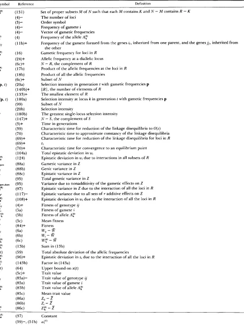
TABLE I

Glossary of symbols

Symbol Reference Definition

Allele i h at locus k

Constant Constant Constant Constant Constant

Gametic covariance of Z and W Genic covariance of Z and W Epistatic covariance of Z and W

Component of epistatic covariance of Z and W due to the interaction of all the loci in R Two-locus recombination frequency

Frequency of reassociation of the genes at the loci in I , inherited from one parent, with the genes at the loci in J ,

Total frequency of recombination

Recombination frequency between loci k and 1 such that k < 1

T h e smallest two-locus recombination frequency

Frequency of reassociation of the genes at the loci in K , inherited from one parent, with the genes at the loci in

Total frequency of recombination among the loci in R

n-locus linkage disequilibrium: the difference between the recombined and unrecombined adult genotypic fre- inherited from the other

R - K , inherited from the other

quencies, weighted by the recombination frequencies and summed over recombination events and one of the gametes

Linkage disequilibrium among all the l o c i in R: defined for R as is D, for N

Linkage disequilibrium among all the loci in R: defined for R as is d, for N

n-locus linkage disequilibrium: the difference between the frequency of gamete i and the product of the corre-

Scaled linkage disequilibrium among all the loci in R

Scaled n-locus linkage disequilibrium

Relative error in the fundamental theorem of natural selection Expectation over the gametic frequencies fi,

Total epistatic deviation in z,

Epistatic deviation in z, due to interactions in all subsets of R Recombination function

Selection function

Selection function for the loci in R Epistatic function

Recombination function

Recombination function for the loci in R Allelic selection function

Allelic selection function

Proper subset of loci { 1, 2, . . . , n 1 including 1

Allelic index at locus k

Gametic index (i,, i ~ . . .

.

, i,)

Vector with components ir for every k in R

N

-

I , the complement of I Gametic index

Constant Subset of R

Locus index Constant Constant Subset of N Locus index

I L 1, the number of elements of L T h e number of alleles at locus k

Constant Subset of N

I M 1, the number of elements of M

{ 1, 2, . . . , n 1, the set of loci

Set of subsets of I of N such that each I contains either k or 1

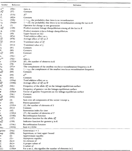
Evolution of Multilocus Systems

Table I-Continued

Symbol Reference

63 1

Definition

Set of proper subsets M of N such that each M contains K and N - M contains R - K The number of loci

O r d e r symbol Frequency of gamete i

Vector of gametic frequencies Frequency of the allele A!:’

Frequency of the gamete formed from the genes i,, inherited from one parent, and the genesj,, inherited from

Gametic frequency for loci in R

Allelic frequency a t a diallelic locus N

-

R , the complement of R

Product of the allelic frequencies at the loci in R Product of all the allelic frequencies

Subset of N

Selection intensity in generation t with gametic frequencies p

IR I, the number of elements of R T h e smallest element of R

Selection intensity a t locus k in generation t with gametic frequencies p

Subset of N Selection intensity

T h e greatest single-locus selection intensity N

-

S, the complement of S

Time in generations

Characteristic time for reduction of the linkage disequilibria to O(s) Characteristic time to approximate constancy of the linkage disequilibria Characteristic time for reduction of the linkage disequilibria for loci in R

t l

Characteristic time for convergence to an equilibrium point Total epistatic deviation in w,

Epistatic deviation in w , due to interactions in all subsets of R Gametic variance in Z

Genic variance in Z Epistatic variance in Z Total genetic variance in Z

Variance due to nonadditivity of the gametic effects on Z Epistatic variance in Z due to the interaction of all the loci in R Epistatic variance due to all sets of r additive effects on Z Epistatic deviation in w, due to the interaction of all the loci in R Fitness of genotype ij

Fitness of gamete i

Fitness of allele A!:’

Mean fitness Fitness

the other

W,] -

w

W, -

w

w!;’

-

w

Sum in (1 3b)

Total absolute deviation of the allelic frequencies

Epistatic deviation in z, due to the interaction of all the loci in R Factor in (1 43a)

Upper bound on x ( t ) Trait value

Trait value of genotype ij

Trait value of gamete i

Trait value of allele A!;’

Mean trait value

Z,]

-

z

z,

-

z

z!;)

-

z

a!:’ (37) Constant

Table I-Continued

Synlbol Reference Definition

max, a,

Constant

p !”

Constant

1

-

c,,,, the probability that there is no recombination

1

-

c!:?, the probability that there is no recombination among the loci in R

Operator for change in one generation

Product-moment linkage disequilibrium among all the loci in R Product-moment n-locus linkage disequilibrium

Upper bound on 1 d, I

Total additive effect on z,

Average effect of A!:’ on 2

Translated value of Gf’ Translated value of 1; Constant

Constant Constant

y ’

maxi K ,

I K 1, the number of elements in K Constant

T h e complement of the smallest two-locus recombination frequency in R

1 - c,,,, the complement of the smallest two-locus recombination frequency

Constant

fl!W Constant

Total additive effect on w , Average effect of A!? on W

Frequency of the allele A!:’ on the linkage-equilibrium surface Frequency of gamete i on the linkage-equilibrium surface Vector of gametic frequencies on the linkage-equilibrium surface Constant

Constant

Sum over all components of the vector i except ik

Fitness parameter

1 S 1, the number of elements of S

Constant

Summation index for time

I T I , the number of elements of T

Recombination function

Indicator function for the allele A!?

Indicator function for gamete iK in K Recombination function

Sum in (161b)

Generation t

+

1

Supremum, or least upper bound Approximate equality

Asymptotic equality An element of A proper subset of A subset of

ILI (1 39)+ For a set L , this signifies the number of elements in L

Evolution of Multilocus Systems 633

for every

k,

ie., the single-locus “linkage disequilibria” are zero. From (1 1 b), (sa), and (5b) we obtain

D, = c,[ W!:)pj:)

-

X!:)(Z)], ( 1 3a)

2 I

where

x!:)(I)

=

c ( ~ )

c

WigJ,j,i,pt,JJ,jli,. (1 3b)

i j

There are two possibilities in (1 3b): either

k

E I or

k

E J . If

k

E I , then (5a) and (5b) yield

X!:’(]) = F k )

c

CC

W*,jJ,j,*JPtlJJpj,tJ

9 JJ I 1 9

Wi, p i l 7

(A) ( 4 .

(14)

a similar argument produces the same result for

k

E

J . Therefore, (1 3a) establishes (12). Summing (1 la)

and appealing to (4), (6c), and (1 2), we find

WAp;:’ = p!:)wl:). (1 5)

Although it is the linkage disequilibria Di that enter the basic recursion relations (1 l ) , a simpler set of linkage disequilibria that do not involve the fitnesses (and which seem not to have been used for more than two loci) will be more convenient for our analysis. As above, suppose R

C

N and Q = N

-

R. Then the gametic frequencies for loci in R read

p!,“’

=

C

p , ;

(16)

iP

of course,

pry

=

p,.

We introduce the linkage disequi- libria

dl,“) =

p1(:)

-

ql:), ( 1 7 4

in which

q 1.Q

(R) =

n

pj;).

(1 7b) kER

In particular, for R = N we have

d . = p . - q I I I ,

( 1 8 4 in which

n

q; =

n

p!;’.

(1 8b)

k= I

T h e analog of (1 2) follows immediately from (1 8) and (4): for every

k,

di = 0. (1 9)

From (1 Ib) and (1 8) we see that if there is no position effect and dl = 0 for every i, then Di = 0 for every i.

We now turn to the definition of the selection intensity s. At least for weak selection, a simple, nat- ural definition is often manifest; for our purposes, definitions of the same order of magnitude are equiv- alent. T o be specific, however, we choose the most

i

conservative definition. We take

as the selection intensity in generation t with gametic frequencies

p

and define

s = sup r ( p , t ) . (20b)

P.1

Observe that (6a), (5c), and (20) give

for every i a n d j , which is equivalent to

Thus,

w l J ( p ? l) = o(s) (22)

as s --., 0. Here and below, unless indicated otherwise, all order symbols are uniform in p and t. If the fitnesses are independent of time, the supremum in (20b) becomes a maximum over the gametic frequen- cies. For constant fitnesses, (20) simplifies to

s = (max,,J W ,

-

minj,l W,J)/min,,j W t J . (23)

An important immediate consequence of (1 5 ) and (22) is that gene frequencies change slowly:

Weak selection will mean s << c,,,~”.

Two examples may illuminate the definition of s.

Consider a single diallelic locus with gene frequency

P .

For the fitness pattern

W11 = 1

+

2u‘, Wl2 = 1

+

u, W22 = 1 , (25)

with u

>

-1, a natural choice for

I

u

1

<<

1 would be s =

I

c

I.

This agrees with (23), from which we easily deduce

( 2 2

-

u)/(l

+

u), u

<

0,

0 S u

c

9’2, (26)

u

>

Y 2 .

T h e large value of s in (26) for u close to

-

1 correctly reflects the fact that the heterozygote is then almost lethal.

For the frequency-dependent fitness pattern

W I I ( ~ ) = 1

+

p

+ 4 4

-

6 p ) , ( 2 7 4

Nagylaki

s = u. Straightforward application of (20) leads to

s = { 3u/(l

+

a), 0

<

u d 5 4 ,

u/(l

-

a), ‘/2

<

u

<

1, (28)

which is indeed of order u for u

<<

1. Note that s +

as u 4 1 because

WIl(1) = Wp(1) = 2(1

-

u) + 0 (29)

as u + 1.

Our last task in this section is to derive a recursion relation for the linkage disequilibria d;. From (18), (24), (1 la), and (22) we obtain

Adi = A p ,

+

O ( S ) (30)

=

-Dl

+

O ( S ) . (31)

Successively invoking (1 lb), (22), (16), and (17), we deduce

Di =

C

cI(

pi

- p i , (0

pi,

0 )

+

O(s) ₍₃₂₎

= cr(di

-

d,, d 9

-

d;,

-

d y q j ; )

+

~ ( s ) . (33)

I

(0 0 (0 0

I

Substituting (33) into (31) and recalling (7) produces the recursion relation

d l = YNdi

+

sJ;(p,

t )

+

g t ( p i ) , ( 3 4 4 where the prime signifies generation t

+

1;

YN = 1 - Ctot (34b) represents the probability that there is no recombi- nation among the loci in N ; the functionf;(p, t ) satisfies

If;(p,

0 1

d PI ( 3 4 4 for some constant pi independent of

p,

t , and s, and

j(p,

t ) is independent o f t if the genotypic fitnesses are

independent o f t ; and

Note that 0

<

Y~

<

1. Our analysis will be based on (15) and (34), rather than on (1 1).

The recursion relation for where R C N, can be written down directly because it must have the form (34), as can be confirmed by observing from (16), (1

7),

and (1 8) that

d R ) ‘ R = d ; , 4:;) = q,

‘e ie

and summing (34a) over ip Thus, we have

in which Y R denotes the probability that there is no recombination in R ; on account of the embedding

R G N , the selection function

still depends on the full vector p of n-locus gametic frequencies; and for suitably defined recombination frequencies in R , the recombination term gl:) has the form (34d).

We shall need (*), however, only for two-locus subsystems. In this case, since dl:) = 0 for every R and

ik by (1 7), therefore (34d) tells us that g!:) = 0, and

hence (*) reduces to

d i t ) ’ = Y R d i f )

+

sfIp(p, t ) , ( 3 5 4 where

I$Ip(p, t )

I

Pl:) (35b)

for some constant pl:) independent of p, t , and s. Now (32) gives

D ( R ) 1R = Dl = ~ ( ~ ’ d l f ’

+

O(s),

(36)

‘Q

where c ( ~ ) = 1

-

Y R designates the recombination frequency between the two loci in R .

REDUCTION O F THE LINKAGE DISEQUILIBRIA

In this section, we demonstrate the rapid reduction of the linkage disequilibria

d i

to O(s). This result is an immediate consequence of the following useful bound. For every subset of loci R G N a n d t = 0, 1, 2,

. . .

, the linkage disequilibria satisfy

I

d!f’(t)

I

f f t R ( R ) A R t

+

p!:)s, ₍₃₇₎ where

CY!;)

and

PI:)

denote constants independent of s

and t , and A R designates the complement of the small-

est two-locus recombination frequency in R.

We note in passing that if there is no selection

(s = 0), then (37) establishes global convergence of the n-locus system to linkage equilibrium at a rate no slower than AIL., where

Ah: = 1 - C”,j,,. (38)

Thus, our proof provides an alternative to the analyses

of GEIRINGER (1944), BENNETT (1954), REIERSOL

(1 962), and LYUBICH (1 97 1).

We define CY, = and CY(’? = max,a,, and let t l

represent the shortest time such that CY(’%$ d s. Then (3 7) implies

di(t) = O(s), t 3 t l

-

(In s)/ln A N , (39)

as s + 0. If cmin

<<

1, we have the approximation t l =:

-c;tn In s, and then t l may be considerably longer than the short time -In s, which will usually not exceed 5 or 10 generations. If the population is initially in linkage equilibrium, i . e . , di(0) = 0 for every i, then

= 0 for every R and iR, so t l = 0. There-

fore, t l should be conservative if the population is initially close to linkage equilibrium:

I

d;(O)

I

<<

1 for every i. From (24) we see that the total gene- frequency change during the time t l is very small, of

Evolution of Multilocus Systems 635

Applying (39) to (30) and (31), we conclude

Api = O ( S ) , t b t l , (40)

D i ( t ) = O ( S ) , t 3 t l . (41)

For two loci, (41) was derived in NAGYLAKI (1976); in this case, its equivalence to (39) is obvious from (36). We shall prove (37) by induction, starting with two embedded loci and then generalizing to an arbitrary number.

Two loci: Iterating (35a) leads to

dj,R'(t) = d!,R'(O)y:,

1- I

where the sum is absent for t = 0. Taking absolute values in (42) and substituting (35b), we get

(43)

For two loci, XR = Y R , so (43) establishes (37).

Multiple loci: We show now that if (37) holds for

every proper subset R C

N ,

then it holds for N .

T o estimate

gi(pJ,

note first from (1

7)

that

lq!:)(t)l d 1, [ d ! t ) ( t ) I G 1. (44)

A glance at (7) to (1 0) confirms the obvious, that cmin

<

ctOt, whence (34b) and (38) yield

A N = max XR

>

YN. (45)

R

Equations 34d and 44 reveal that

I

gi(pi)

I

d

C

~ [ 2

I

d!:

I

+

I

d t )

11.

(46)

I

Using (37) for I C N and J C N and then replacing XI

and X, by A N leads to

I

g i ( p i )

I

d ai&

+

his, ( 4 7 4 where

ai =

2

~ ~ ( 2 4

+

a?), bi =

2

CI(~P~:

+

@?).

(47b)

I I

Substituting (34c) and (47a) into (34a), we obtain

l d / l d ?Nidi[

+

(YiXh

+

Bis, (48)

where B j = p i

+

bi.

NOW consider & ( t ) such that Si(0) =

I

di(0)

I

and

6; = Y N 8 i

+

ai&'

+

&s. (49)

If

1

di(t)

I

d %(t) for some t , then (48) and (49) inform

US that

I

di(t

+

1)

I

d &(t

+

l ) , so we conclude by

induction that

Idi(t)I d $ ( t ) ( 5 0 )

f o r t = 0 , 1 , .

. . .

to (49):

We keep in mind (45) and apply the solution (42)

1- 1

& ( t ) = 6,(0)Yfv

+

y ; y ( a i y r - '

+

B,s)

7-0

ai hfv Bi s

d

&(O)rfv

+

d aJfv

+

p i s , ( 5 1 4

A N

-

YN 1

-

YN

+-

where

( Y j = 6,(0)

+

,

P,=-

.

(51b)

ai Bi

AN

-

YN 1

-

YN

Therefore, (50) and ( 5 la) imply that (37) holds for

R = N , which completes our inductive proof.

A P P R O X I M A T I O N O N T H E L I N K A G E - EQUILIBRIUM SURFACE

For t 2 t l , according to (39), the linkage disequi- libria are O(s), which suggests that the population evolves approximately as if it were in linkage equilib- rium, the difference between the exact gametic fre- quencies and those of the much simpler system on the linkage-equilibrium surface being O(s). To make this precise, recall that the exact gene frequencies

p f : ) ( t )

evolve according to the complicated law (15), which depends on the gametic frequencies

p i .

The gene frequencies r!:)(t) on the linkage-equilibrium surface evolve according to the much simpler law obtained by imposing linkage equilibrium on (1 5). We choose

d f ) ( t I ) = pjf)(t1) (52)

for every

k

and i k ; we shall prove that

p , ( t ) = rl(t)

+

O(s), t l d t 6 K / s , (53a)

as s 4 0, where K designates a constant and

n

7 r i =

n

Ti, ( I ) _(53b)

k= 1

denotes the gametic frequencies on the linkage-equi- librium surface.

If r(t) does not necessarily converge to some equi- librium point or if r(t1) is on the stable mainfold of an unstable equilibrium, then small perturbations may cause large deviations in its ultimate state. In this case, the restriction t d K / s in (53) may be necessary.

For two loci, a different proof of (53) was presented

in NACYLAKI (1977b, pp. 171-173; 1992a, pp. 179-

18 1).

Proof of (53): From (1 Sa) and (39) we obtain

pi(t)

= q t ( t )

+

O ( S ) , t 3 t ~ . (54) In view of (24), we may rewrite (1 5) as

Apl,k’ = sHl,k’(p, t ) ; (55)

because of our assumptions on W+(p,t), the uniformly bounded function Hj:’(p,t) is continuously differenti- able with respect to p. We invoke (54) to expand (55) by Taylor’s theorem:

Ap!:’

= sH$(q, t )

+

s2h!:’(q, t ) , t 3 t l , (56) where

C C

Ih!:’(q,

t)l

C M (57)

k i,

for some constant M independent of q, t , and s. On the linkage-equilibrium surface, (55) becomes

AT!:)

= sH!:’(r, t ) . (58) We put

x ( t ) =

C

c

Ip!:’(t)

-

Tl,k’(t)I

1 (59) k i,

subtract (58) from (56), sum over

k

and ik, and take absolute values to derive

x ( t

+

1) C

[ I

p!:’(t)

-

* $ ( t )

I

k i,

+

s

I

H!:’(q, t )

-

H!:’(r, t )

I

(60)

+

s2

I

h!:’(q, t )

I]-

By Taylor’s theorem, since H!:’(p,t) is uniformly bounded and continuously differentiable with respect to p, there exist constants L$! independent of q, r ,

and t such that

I

H!:’(q, t )

-

H!:’(T, t )

I

c

x

L!::)

I

p!:’(t)

-

$ ( t )

I.

(61)

1 i,

Inserting (59), (61), and (57) into (60) leads to

x ( t

+

1)

e

(1

+

L s ) x ( t )

+

M s 2 , t 3 t l , (62a)

x(t1) = 0, (62b)

L = max _{L!::’ (63)}

where

l.ij k ih and (62b) follows from (52).

Now consider y(t) such that

y ( t

+

1) = (1

+

L s ) y ( t )

+

M s 2 , t 3 t l , (64a)

y(t1) = 0. (64b)

T h e induction argument between (49) and (50) dem- onstrates that

x ( t )

c

y ( t ) , t 3 t l . (65) But (64) yields

y ( t ) =

-

M s [(l

+

LS)”“

-

13 L

C - M s (1

+

LSy

L

which establishes that

~ ( t ) = O ( S ) , tl C t C K / s . (67)

By (65), the same holds for x ( t ) , which proves (53).

SLOW VARIATION O F T H E LINKAGE DISEQUILIBRIA

Here, we posit that the explicit time dependence (if any) of the genotypic fitnesses is O(s‘):

WtJ[p(t), t

+

13

-

w,[p(t), t3 = O(s2) (68)

as s + 0 for every i, j , and t. T h e hypothesis (68) will enable us to prove that after a time t 2

-

2 t l , the

linkage disequilibria are almost constant, their rate of change being O(s2). We shall derive this conclusion from the following useful bound. For every subset of loci R G N , the linkage disequilibria satisfy

I

Adi,“’(t)

I

s ( K ! : ’ A ~ ~

+

pi:’s), t 3 $ 1 , (69)

where K::) and pi:) denote constants independent of s and t.

T h e inequality (69) corresponds to (37). In fact, it

will be clear that (69) holds with tl replaced by t R

-

(In s)/ln AR for each R. We have used tl for simplicity and because our interest centers on R = N and t N

=

t l .

We define K~ = K ! ~ ) and K ( ~ ) = maxzKz, and let t 2 represent the shortest time such that K(‘%%-‘~ s.

Then (69) implies

Adi = O(s‘), t 3 t2

-

t l

+

(In s)(ln AN)-’ (70)

as s + 0. If the population is initially in linkage equilibrium, t l = 0; otherwise, t l

-

(In s)/ln AN, SO t 2

-

2tl as s + 0. T h e time t 2 may be considerably longer than 10 or 20 generations if c,in

<<

1. T h e total gene- frequency change during the period t [

<

t

<

t 2 is very small, of order s ( t g

-

t l )

-

(s Ins)/ln AN, which is approximately the same as during the initial period

( t

e

tl).

Evolution of Multilocus Systems 637 t

s

t s , which, we shall show, is precisely when we

expect generic increase of the mean fitness. Of course, (39) precludes substantial change in the linkage dis- equilibria for t

>

t l .

Observe that (69) and (70) differ from (37) and (39), respectively, essentially by a factor s. This is not surprising: (40) suggests that if explicit time depen- dence is negligible [see (68)], then for t 2 t l , all functions of the gametic frequencies should change at the relative rate s, as if they were functions of st rather than o f t .

T h e estimate (70) is the precise and general state- ment of quasi-linkage equilibrium and w i l l be required for the proof of the asymptotic fundamental and secondary theorems of natural selection. KIMURA (1 965) was the first to argue for two diallelic loci that the linkage disequilibria varied slowly and that this was related to the fundamental theorem of natural selection. T h e result (70) for W D , and the asymptotic fundamental theorem of natural selection were proved for two multiallelic loci in NACYLAKI (1976).

Provided the position effect (if any) is O(s') [see (1 35)], D, also satisfies (70) [see below (148)].

We shall prove (69) by induction, starting with two embedded loci and then generalizing to an arbitrary number.

Two loci: Because of (39), we may set

dl, ( R ) ( t ) = sdl,"'(t), t 3 t l , (71)

where dI:'(t) is uniformly bounded as s + 0. Substi- tuting (71) into (35a), we obtain

dl:)'

= yRd!:' +fi,"'(P, t ) , t 3 t l , (72)

whence

(ad,,

' ( R ) ) I -

-

y R ~ d ! , K '

+

~ f l , " ) ( p , t ) , t 3 t l . (73)

We decompose the change in$ into parts due to its

dependence on the gametic frequencies and on time:

Afi,"'(p, t ) = {fi,"'[p(t

+

I ) , t

+

I ]

-f!,"'[p(t), t

+

111 (74)

+

(fl,R'[p(t), t

+

11 -fi,"'[p(t), t ] ) .

By Taylor's theorem and (40), the expression in the first brace is O(s). Since the selection term in (35a) is

sf!:',

we infer from (68) that the expression in the second brace is also O(s). Therefore, (73) becomes

(Adi, - ( R ) )

-

Y R A ~ ! ~ )

+

O ( S ) , t 3 t l , (75)

I

-

which has the form (35a). Consequently, (43) gives

I

Ad,, ( t )

I

S

I

Adj,"'(t,)

1

7gt1

+

p ! f ' s , t 3 t l , (76) for some constants p!:). Recalling that XR = y R for two loci, we see that (71) and (76) establish (69).

Multiple loci: We demonstrate now that if (69) holds for every proper subset R C N, then it holds for N.

From (34a) we obtain

(Ad,)' = ylvAdi

+

sAJ;(p, t )

+

Agi(pi)*

(77)

Since the argument based on (74) applies to any number of loci, there exist constants A, such that

I

A$(p, t )

I

s

A s . (78)

To estimate Ag,, first we deduce from (34d)

A g i ( p i ) = c ~ I l [ d ~ : A d i j ) + d y A d i : + ( A d i : ) A d y ]

I

+

[di;Aqjf+dyAqi!]

+

[(Ad!:)A$ (79)

+ ( A d y ) A q i : ]

+

[ q y A d ! : + q i : A d ? ] ] .

For t 3 t l , (39), (17b), and (24) inform us that the expressions in the first three brackets are O(s'), and (44) bounds the expression in the last bracket. There- fore, we have

IAgt(p,)l S

C

c~[IAd!:'l

+

I A d y I ]

+

ais'

(80)

I

for t 2 t l and some constants 0,. Employing (69) for

I C N and J C N and then replacing XI and X, by AN

leads to

I

A g l ( p , )

I

s

1~XfiT'l

+

v , s 2 , t 3 t l , ( a l a ) where

11 =

c

cI(Ki:)

+

K ? ) ,

I

(8 1 b)

=

ei

+

cI(pI:)

+

p;j).

I

Inserting (78) and (8la) into

(77),

we find

I

A d ,

1 '

S yay

I

Ad,

I

+

q ~ X ~ ~ ~ 1

+

t 3 t l , (82)

where

r,

= A,

+

ut. By virtue of (39), we may again substitute (7 1) for R = N to obtain

I

A&

I

I

s

y N

I

adi

I

+

Vi~rfl

+

ris,

t 3 t l , (83)

which has precisely the form (48). Therefore, (50)

and (5 1) imply that

I

A d , ( t )

I

S ~,h?l

+

pis, t 3 t l , (84) for suitable constants ~i and pi. In view of (71), this establishes (69) for R = N , which completes our proof.

ANALYSIS OF VARIANCE AND COVARIANCE

rems of natural selection are generically dominated by the genic variance in Wand by the genic covariance of Z and W, respectively, and many results of our analysis will be required to prove these theorems. T h e analysis in this section will involve dynamics only at the end, when we shall invoke (39) to show that the average excess is close to the average effect for each allele, and then use (53) to demonstrate that the

analysis of variance and covariance can be approxi- mated on the linkage-equilibrium surface, where the allelic effects at different loci are independent.

Analysis: Let Zq(p,t) designate the trait value of

genotype ij. We define the mean values of the gamete i, the allele Ai:), and the population by

i

z

= zqpipj. (85c)

i .I

For the deviations from the mean

z,

we have

z , =

z . .

-

g g

z,

@sa)

zi =

zi

-

z

= _{z . . p . r j I ’ (86b)}

P i * ( Z i , ( 8 6 4

Thus, z, and zi:’ signify the average excesses for the character of the gamete i and the allele Ai:), respec- tively.

We decompose the gametic excess zi into an additive effect [, and an epistatic deviation ei,

-

j

pi;’r$

= (k) ( I )

-

z)

z , p l .

i

z, =

5;

+

e i , ( 8 7 4

and then set

n

r i =

c

l!:),

(87b)

k- 1

where

ri:)

denotes the average effect of the allele Ai:’ on the character Z , determined below. Then the ga- metic, genic, and epistatic components of the variance in Z are

Vgam = 2

C

P d ,

(884

i

Vg = 2

C

p i c ? , (88b)

i

V, = 2 p i e : . ( W

We eliminate ei from (88c) with the aid of (87) and minimize V, with respect to {j:). This leads easily to

[$ EWENS (1979), pp. 217-2181

i

CQ)

piei = 0 (89)

for every k and ik. Substituting (87a) into (86c) and

i

using (89) yields

p ! : p

1, =

c

( W

PIS;.

, ,

(90)

1

In (go), there is one equation for each k and ik. T h e

unknown allelic effects {!:) appear only in the sums

li;

summing (89) over i k and using (86b) and (86a), we

infer

C

p i l l = 0 . (91)

I

Let us momentarily translate the average effects ac- cording to

and observe that the choice

ck =

P I ,

( k )

li,

( 4

‘ k

gives

C

Pik ( k ) ‘ ( k )

l t k

-

-

0

.

Ik

Furthermore, (91) and (87b) reveal that

ck = 0 , k

whence J: = fl. Therefore, we may simply assume

pjp{::’

= 0 (92)

Ik

for each k.

deduce

Appealing successively to (88b), (87b), and (go), we

V g = 2

c

pili

c

sf,”’

1 k

= 2

C C

ilk

(k)

C

(k) P i l l

k i, i

= 2 pi;’f!:’z::’. (93)

k i h

From (88a), (87a), (88b), (88c), (87b), and (89), we derive

V p m = 2

2

pi(rt2

+

e2

+

2Ciei)

I

=

vg

+

V ,

+

4

_lj:)

_piei

=

vg

+

v,.

₍₉₄₎

k i, i

Since the gametes are combined in generalized Hardy-Weinberg proportions, therefore V,,, is the additive component of the total genetic variance V in the least-squares decomposition

Evolution of Multilocus Systems 639

Since our analysis is entirely within gametes, domi- nance deviations cannot enter. Therefore, the epis- tatic deviation e, and variance V, involve only the interaction of additive effects, into which w e proceed to decompose them.The reader may find some aspects of BULMER’S (1980, pp. 46-51) panmictic analysis of the diploid variance helpful.

Suppose here that R G N contains at least two loci and put

where xi:) designates the effect of the interaction of all the loci in R . T h e corresponding components of the epistatic variance V, are

vlp’

= 2 p i , ( R ) [Xi, ( R ) ] 2

.

₍₉₇₎

1,

Successive minimization of these variance components for sets R of n , n

-

1 ,

. . .

, 3 loci leads to

pix!:)

= 0 for every

k

E R. (98)

l h

Substituting (96) into (88c) yields

(99)

If R # S, then there exists

k

E R such that

k

4

S, or

k

E S such that

k

4

R. Together with (98), (16), and (97), this fact reduces (99) to orthogonal form:

v,

=

2

x

p l [ x i : ’ ] 2 =

viR’.

(100) R C N i R G N

We remark that (96) and (98) enable us to confirm (89):

in which the inner sum vanishes because R contains at least two loci.

We define the mean deviation e!:) by

P i ,

( R ) e ( R ) I l l = p i e i , (101)

‘Q

in which, as always, Q = N

-

R. Inserting (96) into (1 01) and using (98) and (1 6), we find

whence

Thus, e!:) is the sum of the effects of the interactions

in all the subsets of R. We can rewrite (102) as

X ! R ) = eff

-

x!:),

‘R (103)

SCR

from which, starting with x!,“) = e!:) for subsets of two loci, x!,”’ can be determined recursively as a linear function of the known deviations e!:) with S

C

R.

We turn now to the analysis of covariance. Corre- sponding to (87), we decompose the gametic fitness excess wi into an additive effect ti and an epistatic

deviation ui,

WI = t l

+

ut, (1 04a)

and then set

11

t i =

C

t::),

(1 04b)

it= 1

where

’

[I:

denotes the average effect of A!:) on fitness. We define the gametic, genic, and epistatic covari- ances of Z and W as

Cgam = 2

C

p i z i w i t (1 05a) i

Cg =

2

C

p i r i t z , (1 05b)

1

C, = 2 p i e i u , . (1 05c)

Appealing successively to (105a), (87a), (104a), (87b), (1 04b), (89), and the analog of (89) for u;, we find

I

Cgam = 2

C p , ( f t &

+

e i u 1

+

3;u;

+

e i b ) i

= Cg

+

C ,

+

2

( 1

s!:’

~ ( ‘ ) p , u i

+

t i , p i e i

=

cg+

c,.

( 1 0 6 )

( 9 (1)

k ik i

1

T o justify the term genic covariance, we express Cg

purely in terms of allelic variables. Consecutive use of (105b), (87b), and the analog of (90) for fitness pro- duces

Cg = 2

C

C

r i , ( k )

C

( k ) P i t i

k ib i

=

2

C C

p i , r i k w i ) 9

(k) (k) ( 4 _{(1 07a)}

k i,

which is the covariance of the average effect on the character

(e:))

and the average excess for fitness (wii)) of every allele that affects the character. Observe the

loss of symmetry between 2 and W due to the decom-

position of (105b) into allelic effects. However, apply- ing (104b) and (90) to (105b) yields

Cg = 2

C

_C

P I , z z h

tik

k

1

,

(k) ( k ) ( k )

(1 07b)

it is w!,k) rather than

[j:)

that controls gene-frequency change, (1 07a) is more natural and useful than (1 07b).

T o decompose the epistatic covariance C,, we set

ut = V I ; ' , (108)

RGhT

where v!:) designates the effect on fitness of the inter- action of all the loci in R. We define the corresponding components of C, as

cl."'

= 2

C

p , ,

( R ) ( R ) ( R ) XI, ut,

.

_{( 1 09)}

'H

Substituting (96) and (108) into (105c), utilizing (98) and its analog for vi:) as in the proof of (loo), and employing (16) and (1 09), we deduce

Next, we prove that the average excess zi:' and the average effect

{r:)

differ only because of linkage dis- equilibrium. T o see this, in successive lines we invoke (90) and (87b); (4); (16) and (1

7);

(92); and (39):

= p i h ( 4 ( k )

C;,

+

O(s), t 3 t l ; ₍₁₁₂₎ the sum in the second line above is over all compo- nents of the vector i except z k and

&.

For fitness, (1 11)

holds with z!:) and

{i:)

replaced by w!,k) and

E!:),

respec- tively, but, on account of (22), the approximation (1 12) becomes

p,, ( 4 w,, (k) = p , , (k) (k) E t h

+

O(s'), t 3 t l . (1 13) Finally, we observe that (53) and Taylor's theorem enable us to approximate the variances and covari- ances on the linkage-equilibrium surface. For the var- iance components of Z, (88) gives

V,,,(p, t ) = VPm(r, t )

+ O(S),

ti

s

t K / s , (1 14) and analogous approximations for V, and V,. From (105) we get

C,,(p, t ) = CKam(r, t )

+

O(s2), t l

s

t

s

K / s , (1 15)

and analogous formulas for C, and C,. For the variance components of W , (88) yields

V,,,(p, t ) = Vgam(r, t )

+

O(s"), t l t

s

K / s , (1 16)

and similar expressions for Vg and V,. Of course, the leading terms in (1 14), (1 15), and (1 16) are O( l ) , O(s), and O(s2), respectively.

On the linkage-equilibrium surface, we have a sim- ple expansion of the epistatic variance V , in terms of the components VAv, of the total genetic variance V associated with all sets of r additive effects on Z (NAGYLAKI 1992b):

n

v e ( r , t ) =

2

2'"VAr(r, t ) . (1 17)

r=2

This formula generally does not hold if there is link- age disequilibrium.

EPISTASIS A N D LINKAGE DISEQUILIBRIUM

As stated in the introduction, if fitnesses are additive between loci, the gametic frequencies always converge to a stationary point in linkage equilibrium (KARLIN

and FELDMAN 1970; KARLIN 1978; KUN and LYUBICH

1979). Therefore, it ought to be possible to relate the linkage disequilibria to the epistatic deviations in fit- ness that maintain them (cf. FELSENSTEIN 1965; LANG-

LEY and CROW 1974; HASTINCS 1985, 1986; BARTON

1986). This is accomplished here.

T h e desired relations follow from the equation

Ad, =

W"P,U,

-

D,

+

O(s'), t 3 t l , (1 18) as s + 0, where the linkage disequilibria d i and

D,

are defined by (1 8) and (1 1 b), respectively, and u, repre- sents the epistatic deviation in fitness, defined by (1 04). Recalling (1 O ~ C ) , from (1 18) we obtain imme- diately

2 e,Ad, = @ - I C e

-

2 e,D,

+

O(s2), t 2 t l , ( 1 19)

1

which will provide a simple proof of the asymptotic fundamental and secondary theorems of natural selection.

For two multiallelic loci, (1 18) and (1 19) hold also with

D,

instead of

d i

on the left-hand side (NAGYLAKI 1976).

Suppose the explicit time dependence (if any) of the genotypic fitnesses is sufficiently weak to satisfy (68). Then (1 18) and (70) give

D i ( t ) = I P p i u *

+

O(s'), t 3 t 2 . (120)