Copyright1999 by the Genetics Society of America
Temporal and Multiple Quantitative Trait Loci Analyses of Resistance to
Bacterial Wilt in Tomato Permit the Resolution of Linked Loci
B. Mangin,* P. Thoquet,
†J. Olivier
†and N. H. Grimsley
†*Unite´ de Biome´trie et Intelligence Artificielle, INRA, 31326 Castanet-Tolosan, France and†Laboratoire de Biologie Mole´culaire des Relations Plantes-Microorganismes, CNRS-INRA, 31326 Castanet-Tolosan, France
Manuscript received May 29, 1998 Accepted for publication November 16, 1998
ABSTRACT
Ralstonia solanacearum is a soil-borne bacterium that causes the serious disease known as bacterial wilt in many plant species. In tomato, several QTL controlling resistance have been found, but in different studies, markers spanning a large region of chromosome 6 showed strong association with the resistance. By using two different approaches to analyze the data from a field test F3population, we show that at least
two separate lociz30 cM apart on this chromosome are most likely involved in the resistance. First, a temporal analysis of the progression of symptoms reveals a distal locus early in the development of the disease. As the disease progresses, the maximum LOD peak observed shifts toward the proximal end of the chromosome, obscuring the distal locus. Second, although classical interval mapping could only detect the presence of one locus, a statistical “two-QTL model” test, specifically adapted for the resolution of linked QTL, strongly supported the hypothesis for the presence of two loci. These results are discussed in the context of current molecular knowledge about disease resistance genes on chromosome 6 and observations made by tomato breeders during the production of bacterial wilt-resistant varieties.
B
ACTERIAL wilt (BW) caused by Ralstonia solana- show symptoms, their vascular systems are neverthelessinvaded to varying extents by the bacterium (Grimault
cearum is a very important disease worldwide,
at-tacking many different species, including many agricul- andPrior 1993). The use of molecular markers and
interval mapping is a powerful approach that permits turally important crops. As the bacterium is soilborne
and enters the plant via the roots, subsequently spread- the identification and genetic mapping of loci
control-ling a trait of interest. Several quantitative trait loci ing in the vascular system, chemical control of the
dis-(QTL) have been shown to play a role in resistance to ease is impractical and environmentally unacceptable.
BW in different studies using different populations and Polygenic resistance has been described in a number
at different geographic locations (Danesh et al. 1994;
of species (Kelman1953 and references therein), but
Grimaultet al. 1995;Thoquetet al. 1996a,b). In studies little is known about the molecular mechanisms of this
using molecular markers, one QTL with a broad LOD type of resistance. Plant resistance to pathogens in
vari-peak on chromosome 6 was of overriding importance. ous interactions is sometimes associated with a
hypersen-However, the map position of the maximum LOD score sitive response (HR), a phenomenon often controlled
observed on chromosome 6 differed between popula-by single dominant loci, and some of the genes
control-tions and between environments. Here, by temporal ling this type of response (R-genes) have been cloned
analysis of disease development and use of two different
and characterized (seeBakeret al. 1997;De Wit1997;
kinds of statistical analyses, we show that there are most
Gebhardt 1997; Hammond-Kosack and Jones 1997
probably at least two QTL present on chromosome 6. for examples of recent reviews). However, there is no
clear genetic evidence that HR is necessary for resistance to R. solanacearum, although a kind of HR has been
MATERIALS AND METHODS
observed in some interactions and may be found in
some plant accessions that also show resistance (Carney Plant growth and inoculation withR. solanacearum:The F
3
pop-andDenny1990;Arlatet al. 1994). In the genus Lyco- ulation ofz3500 individuals was obtained from a cross between
persicon, several accessions of tomato (Lycopersicon escu- Hawaii7996 (L. esculentum, resistant) and WVa700 (L.
pimpinel-lifolium, susceptible) and was planted in the field in
random-lentum) and its close relatives show resistance to BW
ized blocks (Thoquetet al. 1996b). Bacteria (strain GMI8217;
(Wang et al. 1996). Although resistant plants do not
A. Trigalet,personal communication) resistant to streptomy-cin and rifampistreptomy-cin (a derivative of GT1;PriorandSteva1990) were grown as previously described (Thoquetet al. 1996a), and the plants were inoculated under shade cover, using 2 ml of
Corresponding author: N. H. Grimsley, Laboratoire de Biologie
Mole´c-bacterial suspension per plant. Plants were kept under shade for ulaire des Relations Plantes-Microorganismes, CNRS-INRA, B.P. 27
a further 2 days before transfer to an infested field. Auzeville, 31326 Castanet-Tolosan, France.
E-mail: [email protected] Notation of disease symptoms:The development of disease
symptoms was noted about every 2 days after the first signs of tently estimated (EfronandTibshirani1993, p. 307). In our case, the distribution chosen for the Monte Carlo simulation symptom development, from 6 days after inoculation (d.a.i.)
onward. A scale of 1 to 9 was used (Thoquetet al. 1996b). is a mixture of three normal distributions. Deviation from normality has been studied byDoergeandRebai(1995) for
Molecular and genetic analyses:Molecular RFLP analysis
was done as previously described (Thoquet et al. 1996a), the detection of one QTL. Apparently even when the observa-tions follow a skewed distribution, the assumption of normality and marker maps were established both with MAP-MAKER
(Lander et al. 1987) and with JoinMap (Stam1993), using does not materially change the threshold. But, because the information matrix is singular, the QTL parameters are not the Haldane mapping function. Small differences in linkage
distances were found between these maps, so further QTL consistently estimated when the QTL have medium or small effect (Manginet al. 1994), so the threshold obtained by this analyses were performed using MAPMAKER distances because
these are estimated by maximum likelihood. procedure cannot be proven to lead to a correct type I error.
Threshold by intensive Monte Carlo simulations:Goffinet For the purposes of this study, plants were scored either as
healthy (stage 1 or 2) or wilted (stages 3 to 9). The proportion andMangin(1998) propose that the threshold be computed by simulating all of the possible values of the nuisance parame-of plants wilted for each family, x, was then used, after
transfor-ters. The nuisance parameters are varying in a continuous mation using y5arcsin√x to improve the normality of the
space, and even if simulations involve only a limited number distribution, as the statistic for QTL analysis. A few F3families
of points, this procedure needs intensive simulations. How-were poorly represented due to poor seed set or germination,
ever, the threshold obtained leads to a correct type I error. or to bad weather conditions during the test (tropical
thunder-Threshold by stratified shuffling:Stratified shuffling as pro-storms). Arbitrarily, families with ,10 representatives were
posed byChurchillandDoerge(1996) is another possible not used, leaving 187 families for the analysis (the average
way for computing a threshold for the 2QM test. The main family size was 19.0 individuals). Interval mapping was used
step of this procedure is to split up the data with respect to to locate QTL in the F3population, using both MAPMAKER
the assigned classes given by an informative marker and to and MapQTL (van OoijenandMaliepaard1996).
Multiple-shuffle the data in each class. The shuffling is repeated N QTL model (MQM) was performed with the MapQTL
soft-times and the 2QM test is computed for each shuffled data ware.
set. The N test values are used to produce an empirical
thresh-Test for two linked QTL:Using backcross progenies,
Gof-old value at the marker (seeappendix afor more details). finetandMangin(1998) studied tests that permit
discrimina-The stratified shuffling procedure produces a new data set tion between the hypotheses of one or more than one QTL
that behaves asymptotically like a random sample drawn out in a linkage group. Among all the tests compared, the
so-of a population where only one QTL located at the marker called “two-QTL model” (2QM) was the most powerful test
segregates (seeappendix b). for detection of closely linked QTL.
Let us denote by lˆi the empirical threshold obtained at The 2QM test is the minimum value of two statistics,
de-marker i. The stratified shuffling procedure is repeated for noted T(tˆ1) and T(tˆ2), that are obtained by comparing the
each fully informative marker, and an empirical threshold for likelihood maximized under the two-QTL model with the
the whole linkage group, notedlˆ, is obtained by likelihood maximized under the one-QTL model with QTL
position fixed at tˆ1and tˆ2, where tˆ1and tˆ2are the
maximum-l
ˆ 5sup i
lˆi. likelihood estimators of the parameter positions t1and t2from
the two-QTL model. T(tˆ1) and T(tˆ2) are calculated here as
Theoretically, the use of this supremum is not sufficient to LOD tests (difference of the log10-likelihood), like
maximum-guarantee a correct type I error for the test over the whole likelihood ratio tests (two times the difference of the Napierian
linkage group because only positions corresponding to fully logarithm of the likelihood). The mixture likelihood is
ap-informative markers are investigated, but a slight modification proximated by a linear-likelihood approximation that is
well-can be proposed to handle this problem. Before shuffling, known to be effective when the QTL is not a major gene
each individual that is not assigned to a class with certainty is (HaleyandKnott1992;Rebaiet al. 1994), and the
maximiza-assigned to a class by a random draw. The class probabilities tion under the two-QTL model is limited to QTL belonging
for this random draw are inferred for each individual using to nonadjacent intervals.
all of its linked marker information, as are inferred the QTL Let T be the 2QM test; evidence for the presence of more
genotype probabilities in the interval mapping method. How-than one QTL in the linkage group is obtained if T is greater
ever, because only chromosomal locations with markers are than a threshold l chosen such that Pr(T . l) # a for all
investigated, there is no guarantee that the whole procedure possible parameters included in the null hypothesis that there
provides a correct type I error between widely spaced markers. is only one QTL in the linkage group. In F2 progenies, five
nuisance parameters are involved in the null hypothesis:m(the global mean), s2 (the variance), and parameters a, d, t (the
additive effect, dominance effect, and position of the QTL). RESULTS
In fact, there is no problem with the global mean and the
variance because T is invariant for these two parameters, but A molecular map of chromosome 6 was developed
this is not the case for parameters concerning the QTL; more- previously using an F2 population of 200 individuals over, the distribution of T depends on the values of the other from the cross Hawaii79963WVa700 (Thoquetet al. parameters (GoffinetandMangin1998).
1996a). For the purposes of this study, only codominant
Threshold by parametric bootstrap:The simplest way to get
RFLP probes were used, and two further probes, Cf-2
a threshold is to estimate the nuisance parameters in a
one-QTL model and to perform a Monte Carlo simulation with and TG406, were placed on the map (Figure 1, left).
these estimates. This sampling procedure is called a paramet- Cf-2, a cDNA clone containing the coding sequence of
ric bootstrap. the Cf-2 disease resistance gene (Dixon et al. 1996),
This procedure can be shown, by the use of central limit
showed a remarkably high level of polymorphism
be-theorems, to give an asymptotically correct threshold if the
tween the parental lines (10/14 enzyme/probe
combi-observations follow the distribution chosen for the Monte
Figure 1.—Analysis of resistance by interval and MQM scans of chromosome 6. LOD score curves (hori-zontal axes) of resistance to bacterial wilt are dis-played. Markers are shown on the left (map distances on vertical axes in centi-morgans). The LOD score curves are shown at differ-ent times after inoculation (d.a.i.) with the pathogen: 6 d.a.i., fine dashed lines; 14 d.a.i., thick dashed lines; 21 d.a.i., fine solid lines; 28 d.a.i., thick solid lines. The three panels represent d i f f e r e n t t r e a t m e n t s of the data: (A) interval map-ping; (B) MQM cofactor on TG118; (C) MQM cofac-tor on TG240.
bands present), considering the low overall level of poly- In summary, the position of the maximum LOD score
varies considerably over the time course of the
experi-morphism in the population (Thoquet et al. 1996a).
Four different RFLP bands were mapped to the same ment, and suggests that two separate loci might be
affect-ing the resistance. Cofactor analysis (JansenandStam
genomic location, as expected for a multi-gene family
(Dixonet al. 1996). Alleles detected by the probe TG406 1994;van OoijenandMaliepaard1996) was therefore used in conjunction with the above temporal analysis were previously shown to map to chromosomes 3 and
6 (Tanksley et al. 1992), but in our material we did to investigate the possible presence of more than one QTL on the chromosome. Placing a cofactor on TG118 not observe any polymorphism for the chromosome 3
allele. We chose to include the chromosome 6 locus in at 12 cM, corresponding to the maximum of the peak
observed at the end of the resistance test, does not the current study because it improves the map density
in a region close to one of the LOD curve peaks observed support a hypothesis for the presence of two QTL
be-cause the LOD score increase on the distal part of the (see below).
Temporal analysis of disease resistance:When wilting chromosome is insufficient (Figure 1B), in agreement
with the previous results of interval mapping (Thoquet
symptoms were fully developed at 28 d.a.i., a broad
QTL LOD peak associated with many of the markers et al. 1996b). However, the preceding temporal analysis
indicates that this interpretation might be misleading,
on chromosome 6 was observed (Thoquetet al. 1996b;
Figure 1A, 28 d.a.i.). because at 14 d.a.i., the maximum LOD score of 8.1 is
However, the current analysis revealed that as early as 6 d.a.i. several markers showed significant associa-tion with resistance (Figure 1A). The disease then pro-gressed rapidly in the population, and at 12 d.a.i. two regions of the chromosome, between Cf-2 and TG153, and between CP18 and TG406, showed clear association with resistance, with LOD score peaks ranging from 4.3 to 5.9, respectively. Figure 2 shows the temporal progression of the LOD score at these two chromosomal locations. At 14 d.a.i. (Figures 1 and 2), the interval TG73 to TG406 showed the highest LOD score (8.1 at 36 cM), and markers on the upper part of the chromo-some also showed increased LOD scores. Thus, at three different temporal observation points the LOD score of the distal peak exceeded that of the proximal peak (Figure 2). Subsequently, however, the upper part of
Figure 2.—Temporal development of the association of
the chromosome showed the strongest association with two genomic regions of chromosome 6 with resistance. The
resistance, with a plateau exceeding LOD 7 (maximum peak close to TG118 is represented by the solid line, while
the dashed line represents the peak close to TG240.
Figure 3.—Empirical threshold values, for a type I error of 1%, by Monte Carlo simulations over 1000 repli-cates. Points for each LOD (vertical axis) threshold curve were calculated every 10 cM (horizontal axis) us-ing different parameters: fine dashed lines, percent-age of residual variance 5 0.3; fine solid lines, percent-age of residual variance 5 0.2; thick solid lines, per-centage of residual vari-ance50.1. The symbols show the results of assuming d5 0 (h), a 50 (n), or d5a (s). The straight line indicates the 2QM LOD value for the original data (arrow).
observed at 36 cM close to marker TG240. The chromo- located every 10 cM on the chromosome and with the
variance explained by the QTL (a2/21d2/4) ranging
some was therefore scanned using MQM by placing
cofactors on each marker along the length of the chro- from 10 to 30% of the residual variance were done
(Figure 3). The empirical threshold value obtained by mosome in a series of analyses. Use of TG240 as a
cofac-this procedure (the maximum of all of the threshold tor confirmed the likely presence of two QTL on this
values) was 4.04. chromosome, because in this case at both 21 and 28
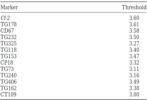
The stratified shuffling procedure gave an empirical
d.a.i. the LOD score rises by.4 LOD units toward the
threshold value of 3.61 (Table 1). Thus, using the test top end of the chromosome (Figure 1C).
value and the thresholds obtained above, we accept with
A statistical test for the presence of two QTL on
.99% confidence that at least two QTL are involved in
chromosome6:Statistical tests that tackle the question
chromosome 6. The maximum-likelihood estimators of of whether one or two QTL might be involved in the
the positions were found near Cf-2 (at precisely 0.7 cM segregation of a particular character have been
com-to the right of Cf-2) and on TG73. These loci explained
pared (GoffinetandMangin1998). Among those tests
12 and 13% of the phenotypic variation, respectively, compared, 2QM was found to be the most powerful in
and their effects were essentially additive. many situations, and this was thus applied using the
data collected 28 d.a.i. At this stage, standard interval mapping could not resolve the presence of two QTL
DISCUSSION
on chromosome 6. The 2QM gave a LOD score of 4.36
for the presence of two loci. Using data collected at the end of the resistance test,
To confirm that the segregation of resistance ob- Thoquetet al. (1996a,b) concluded that there was an
served is most likely due to the presence of two loci, important QTL on chromosome 6 carried by the
various simulations using those constraints imposed by Hawaii7996 parent; their analysis showed clearly that
our dataset (map distances, population size; see below) the LOD curve peak was very broad, but only one locus
were done. These simulations gave the distribution of was identified. Indeed, we confirm here that if only the
the values of the LOD scores that could be obtained in end of test results is taken into account, even use of the
the 2QM by chance, using the given constraints and MapQTL cofactor approach fails to support a hypothesis
assuming the presence of only one QTL. For each simu- for the presence of a second QTL. However, we now
lation, 1000 replications were performed, and the em- present several lines of evidence that indicate that at
pirical threshold value for the test of at least two QTL least two loci controlling BW resistance are present on
vs. one QTL, with a type I error of 1%, was obtained. this chromosome.
The nuisance parameter estimates, needed for the para- Temporal analyses of data collected from F3families
metric bootstrap procedure, were computed using MAP- tested in the field show changes in the maximum LOD
MAKER/QTL (sˆ 5 0.037, tˆ 5 0.108, aˆ 5 0.157, dˆ 5 score peaks during the course of the resistance test. A
0.012). An empirical threshold value of 3.52 was obtained. maximum around 40 cM is clearly observed and
TABLE 1 in resistance. A cofactor placed on or near TG240 re-veals the presence of a second QTL in the upper region
Empirical threshold values, for a type I error of 1%, by
of chromosome 6 in all of the analyses of the F3
popula-the stratified shuffling procedure over 1000 replicates
tion done from 12 to 30 d.a.i., whereas a cofactor placed on a proximal locus (in the uppermost 12 cM of the
Marker Threshold
linkage group) reveals the presence of a second locus
Cf-2 3.60
around TG240, albeit only in some analyses (Figure 2B,
TG178 3.61
14 d.a.i.). The 2QM test indicates with .99%
confi-CD67 3.58
dence that two loci exist near markers Cf-2 and TG73
TG232 3.50
at the end of the test done on the F3population.
TG325 3.27
TG118 3.40 A first indication of the importance of a locus on
TG153 3.47 chromosome 6 in resistance to BW came from breeders
CP18 3.32 who had difficulty combining the resistance to BW with
TG73 3.11
resistance to nematodes conferred by the gene Mi (
Gil-TG240 3.16
bertandMcGuire1956), and this observation has
sub-TG406 3.49
sequently been substantiated in different lines of tomato
TG162 3.38
(P. Deberdt, G. Anaı¨sandP. Prior,personal
commu-CT109 3.00
nication). Because the map location of Mi is known (Klein-Lankhorstet al. 1991;Hoet al. 1992;Weideet
al. 1993) and lies very close (van Wordragen et al.
the end of the test the maximum LOD score is associ- 1996) to the resistance gene Cf-2 (placed on our map),
ated with markers on the top part of the chromosome. the latter being a gene conferring resistance to the
fun-Although individual QTL may contribute different gus Cladosporium fulvum (Dixon et al. 1995, 1996), it
amounts to explaining the variance in different tests or seems likely that several different sources of resistance
at different times during a test, the map positions of to BW carry a locus in this region. Several other genes
real QTL are not expected to move along the chromo- encoding resistance to pathogens have been localized
some. Two possible hypotheses can be proposed to ac- to this chromosomal region (van der Beeket al. 1994;
count for this paradoxical observation of the apparent Williamson et al. 1994;Zamir et al. 1994;Kaloshian
movement of QTL: (1) Because we can only estimate et al. 1995;Sandbrinket al. 1995;Chagueet al. 1997).
the most likely position of a QTL from the available Possible biological explanations for this observation are
data with a certain level of confidence for a particular very speculative, but might arise due to common aspects
map interval, it is possible that this position varies be- of the disease response mechanism, because such
re-tween datasets, and the observations can be explained sistance genes may rely on common kinds of signal
by one QTL; (2) two linked QTL could be involved to transduction pathway (Bonas andVan den
Ackerve-different extents at Ackerve-different stages in the development ken 1997;De Wit1997; Gebhardt1997;
Hammond-of disease. We strongly favor the latter hypothesis be- Kosack and Jones 1997), or on the ability of certain
cause (i) the apparent movement of the maximum LOD genomic regions to generate the variation needed for
score is not random but progresses mainly in one direc- rapid evolution of resistance (Parniskeet al. 1997;Song
tion, and (ii) this shift occurs over a relatively large et al. 1997; Thomas et al. 1997). This BW resistance
map distance (z25 cM; Figure 2). Taken together, the locus, on the upper part of chromosome 6, is therefore
observed data thus constitute a strong argument in favor probably different from the locus carried by tomato line
of the presence of at least two different loci on chromo- L285 (Daneshet al. 1994), because the latter maps close
some 6. Any biological explanation of the shift in the to CT184, atz40 cM on tomato chromosome 6. On the
importance of these loci is speculative. However, the reference tomato map produced from an interspecific
presence of a second locus might possibly be dependent cross of tomato with the wild relative L. pennellii (Tanksley
on environmental conditions such as the presence of et al. 1992), CT184 and TG240 are both located at the
natural light, or on the physiological state of the plant, same map position, 38 cM, and it is therefore likely
because no evidence for a second locus could be found that the QTL from L285 and one of the QTL from
by a similar temporal and statistical analysis (unpub- Hawaii7996 map close to this position. Because this
lo-lished data) of an F2population of cuttings testing in a cus is .30 cM away from Mi, it is most likely to be a
growth chamber, where the markers TG118 and CP18 separate locus to that inferred previously by plant
breed-showed the strongest associations with resistance (Tho- ers to be close to Mi, because it should easily be possible
quetet al. 1996a). to obtain recombinants over such a large map distance.
Two different kinds of statistical analysis, cofactor However, data collected by breeders on the linkage of
analysis (van Ooijen and Maliepaard 1996) and a the locus sp (a morphological marker) to BW resistance
2QM test (Goffinet andMangin1998), show that at from the line HES 5808-2, a descendant of PI 127805A
De Wit, P. J. G. M.,1997 Pathogen avirulence and plant resistance: distal locus, because sp is located near the bottom end
a key role for recognition. Trends Plant Sci. 2: 452–458.
of chromosome 6, close to CT109 in our material (Tho- Dixon, M. S., D. A. Jones, K. Hatzixanthis, M. W. Ganal, S. D.
Tanksleyet al., 1995 High-resolution mapping of the physical
quetet al. 1996a), and is thus too distant (.50 cM) to
location of the tomato Cf-2 gene. Mol. Plant-Microbe Interact. detect linkage with the proximal locus. The accession
8:200–206.
PI 127805A was used as a source of resistance in Hawaii Dixon, M. S., D. A. Jones, J. S. Keddie, C. M. Thomas, K. Harrison
et al., 1996 The tomato Cf-2 disease resistance locus comprises
tomato breeding programs (Acosta et al. 1964) and
two functional genes encoding leucine-rich repeat proteins. Cell may be a progenitor for some of the BW resistance
84:451–459.
found in Hawaii7996. All of these observations lend Doerge, R. W.,andR. Rebai,1995 Significance threshold for QTL
interval mapping tests. Heredity 76: 459–464. further weight to the notion that there are at least two
Efron, B.,andR. J. Tibshirani,1993 An Introduction to the Bootstrap.
QTL controlling BW on chromosome 6. In conclusion,
Chapman & Hall, New York.
there is evidence for one resistance locus close to Mi Gebhardt, C.,1997 Plant genes for pathogen resistance—variation
on a theme. Trends Plant Sci. 2: 243–244. in Hawaii7996, and evidence for a second locus in the
Gilbert, J. C.,andD. C. McGuire,1956 Inheritance of resistance
region of TG73/TG240/CT184 in tomato lines Hawaii
to severe rootknot from M. incognita in commercial-type tomatoes.
7996 and L285. Although these QTL have been ob- Proc. Am. Soc. Hort. Sci. 68: 437–442.
Goffinet, B.,andB. Mangin,1998 Comparing methods to detect
served in different tomato lines and under different
more than one QTL on a chromosome. Theor. Appl. Genet. 96: experimental environments, it is not yet clear how
gen-628–633.
eral these resistances are. The resistance carried by L285 Grimault, V.,andP. Prior,1993 Bacterial wilt resistance in tomato
associated with tolerance of vascular tissues to Pseudomonas sola-close to CT184 is probably specific for certain bacterial
nacearum. Plant Pathol. 42: 589–594.
strains (Danesh andYoung1994). Further work is
re-Grimault, V., P. PriorandG. Anais,1995 A monogenic dominant
quired to map these loci more precisely, to define resistance of tomato to bacterial wilt in Hawaii7996 is associated
with plant colonization by Pseudomonas solanacearum. J. Phytopa-whether or not more than two QTL are present on
thol. 143: 349–352. chromosome 6, and to clarify the biological nature of
Haley, C. S.,andS. A. Knott,1992 A simple regression method
these resistances. To this end, the development of re- for mapping quantitative trait loci in line crosses using flanking
markers. Heredity 69: 315–324.
combinant inbred lines (P. HansonandC. Balatero,
Hammond-Kosack, K. E.,andJ. D. G. Jones,1997 Plant disease
personal communication) will provide an invaluable
resistance genes. Annu. Rev. Plant Physiol. 48: 575–607.
tool for future analyses. Ho, J. Y., R. Weide, H. M. Ma, M. F. van Wordragen, K. N. Lambert
et al., 1992 The root-knot nematode resistance gene (Mi) in We thank the laboratories of Steve Tanksley, Christiane Gebhardt,
tomato—construction of a molecular linkage map and identifica-and Jonathan Jones for supplying RFLP probes, identifica-and Christian Boucher
tion of dominant cDNA markers in resistant genotypes. Plant J. for reading the manuscript. The Region Midi-Pyre´ne´es and the Euro- 2:971–982.
pean Community provided part of the financial support (grant nos. Jansen, R. C.,andP. Stam,1994 High resolution of quantitative traits 3172A and CIP CT 840050 to N.G.). into multiple loci via interval mapping. Genetics 136: 1447–1455.
Kaloshian, I., W. H. LangeandV. M. Williamson,1995 An
aphid-resistance locus is tightly linked to the nematode aphid-resistance gene,
Mi, in tomato. Proc. Natl. Acad. Sci. USA 92: 622–625.
Kelman, A.,1953 The Bacterial Wilt Caused by Pseudomonas
solana-LITERATURE CITED
cearum, Tech. Bul. No. 99. North Carolina Agricultural
Experi-Acosta, J. C., J. C. GilbertandV. L. Quinon,1964 Heritability of ment Station, Raleigh, NC.
bacterial wilt resistance in tomato. Proc. Am. Soc. Hort. Sci. 84: Klein-Lankhorst, R., P. Rietveld, B. Machiels, R. Verkerk, R. Weide 455–462. et al., 1991 RFLP markers linked to the root knot nematode
resis-Arlat, M., F. Van Gijsegem, J. C. Pernollet, J. C. HuetandC. A. tance gene Mi in tomato. Theor. Appl. Genet. 81: 661–667.
Boucher,1994 PopA1, a protein which induces a hypersensi- Lander, E. S., P. Green, J. Abrahamson, A. Barlow, M. J. Daly
tive-like response on specific petunia genotypes, is secreted via the et al., 1987 MAPMAKER: an interactive computer package for Hrp pathway of Pseudomonas solanacearum. EMBO J. 13: 543–553. constructing primary genetic linkage maps of experimental and
Baker, B., P. Zambryski, B. StaskawiczandS. P. Dineshkumar,1997 natural populations. Genomics 1: 174–181.
Signaling in plant-microbe interactions. Science 276: 726–733. Mangin, B., B. GoffinetandA. Rebai,1994 Constructing
confi-Bonas, U.,andG. Van den Ackerveken,1997 Recognition of bacte- dence intervals for QTL location. Genetics 138: 1301–1308.
rial avirulence proteins occurs inside the plant cell: a general Parniske, M., K. E. Hammond-Kosack, C. Golstein, C. M. Thomas, phenomenon is resistance to bacterial diseases? Plant J. 12: 1–7. D. A. Jones et al., 1997 Novel disease resistance specificities
Carney, B. F.,andT. P. Denny,1990 A cloned avirulence gene from result from sequence exchange between tandemly repeated genes
Pseudomonas solanacearum determines incompatibility on Nicotiana at the Cf-4/9 locus of tomato. Cell 91: 821–832.
tabacum at the host species level. J. Bacteriol. 172: 4836–4843. Prior, P.,andH. Steva,1990 Characteristics of strains of
Pseudomo-Chague, V., J. C. Mercier, M. Guenard, A. DecourcelandF. Vedel, nas solanacearum from the French West Indies. Plant Dis. 74:
1997 Identification of RAPD markers linked to a locus involved 13–17.
in quantitative resistance to TYLCV in tomato by Bulked Segregant Rebai, A., B. GoffinetandB. Mangin,1994 Approximate threshold Analysis. Theor. Appl. Genet. 95: 671–677. of interval mapping tests for QTL detection. Genetics 138: 235–240.
Churchill, G. A.,andR. W. Doerge,1996 Permutation tests for Sandbrink, J. M., J. van Ooijen, C. C. Purimahua, M. Vrielink, R.
multiple loci affecting a quantitative character. Genetics 142: Verkerket al., 1995 Localization of genes for bacterial canker 285–294. resistance in Lycopersicon peruvianum using RFLPs. Theor. Appl.
Cierco, C.,andB. Mangin,1996 Construction of confidence inter- Genet. 90: 444–450.
vals for QTL location in F2populations. Biometrics 52: 1268–1282. Song, W. Y., L. Y. Pi, G. L. Wang, J. Gardner, T. Holstenet al.,
Danesh, D.,andN. D. Young,1994 Partial resistance loci for tomato 1997 Evolution of the rice Xa21 disease resistance gene family.
bacterial wilt show differential race specificity. Tomato Genetics Plant Cell 9: 1279–1287.
Cooperative Report 44: 12–13. Stam, P.,1993 Construction of integrated genetic linkage maps by
Danesh, D., S. Aarons, G. E. McGillandN. D. Young,1994 Ge- means of a new computer package—JoinMap. Plant J. 3: 739–744.
netic dissection of oligogenic resistance to bacterial wilt in tomato. Tanksley, S. D., M. W. Ganal, J. P. Prince, M. C. Devicente,
M. W. Bonierbaleet al., 1992 High density molecular linkage
maps of the tomato and potato genomes. Genetics 132: 1141– APPENDIX B 1160.
Thomas, C. M., D. A. Jones, M. Parniske, K. Harrison, P. J. Balint- The asymptotic distribution of Y *iis the distribution
kurti et al., 1997 Characterization of the tomato Cf-4 gene function of an n sample with one QTL located at the
for resistance to Cladosporium fulvum identifies sequences that
ith marker givenuˆi5 uˆi(y),mˆ5 mˆ (y),sˆ25 sˆ2(y), where
determine recognitional specificity in Cf-4 and Cf-9. Plant Cell 9:
u
ˆi,mˆ , andsˆ2are, respectively, the maximum-likelihood
2209–2224.
Thoquet, P., J. Olivier, C. Sperisen, P. Rogowsky, H. Laterrot estimators for the QTL effect at the marker i (additivity
et al., 1996a Quantitative trait loci determining resistance to 1
dominance in backcross, additivity and dominance bacterial wilt in tomato cultivar Hawaii7996. Mol. Plant-Microbe
in F2), the mean, and the variance, anduˆi(y),mˆ (y), and
Interact. 9: 826–836.
Thoquet, P., J. Olivier, C. Sperisen, P. Rogowsky, P. Prioret al., sˆ2(y) are their estimated value for the initial data set.
1996b Polygenic resistance of tomato plants to bacterial wilt in
We focus our attention on a backcross population, the French West Indies. Mol. Plant-Microbe Interact. 9: 837–842.
but similar results could be found in an F2population.
van der Beek, J. G., G. PetandP. Lindhout,1994 Resistance to
powdery mildew (Oidium lycopersicum) in Lycopersicon hirsutum is Working in an asymptotic and local framework for the controlled by an incompletely dominant gene Ol-1 on chromo- QTL effect, as the number of observations tends to some 6. Theor. Appl. Genet. 89: 467–473.
infinity, the effect of the allele substitution, noted a
van Ooijen, J. W.,andC. Maliepaard,1996 MapQTL (tm) Version
3.0: Software for the Calculation of QTL Positions on Genetic Maps. multiplied by
√
n, tends to a finite constant d. This isDLO-Centre for Plant Breeding and Reproduction Research, Wa- the correct framework in which to study the asymptotic geningen, The Netherlands.
distributions of the likelihood ratio test for QTL that van Wordragen, M. F., R. L. Weide, E. Coppoolse, M. Koornneef
andP. Zabel,1996 Tomato chromosome 6: a high resolution are not major genes. In this framework, we get
asymptot-map of the long arm and construction of a composite integrated ically sufficient statistics, which aremˆ , the global mean, marker-order map. Theor. Appl. Genet. 92: 1065–1072. s
ˆ2, the classical estimator of the variance, and the mean
Wang, J. F., P. M. HansonandJ. A. Barnes,1996 Preliminary results
class difference at each marker Sj; j51 . . . I,
of worldwide evaluation of international set of resistance sources to bacterial wilt in tomatoes. Bacterial Wilt Newsl. 13: 8–10. Weide, R., M. F. Van Wordragen, R. K. Lankhorst, R. Verkerk, C.
Hanhartet al., 1993 Integration of the classical and molecular
linkage maps of tomato chromosome 6. Genetics 135: 1175–1186. Sj5
√
n2
1
o
kYkI[Mj,k5A]
o
kI[Mj,k5A]2
o
kYkI[Mj,k5B]o
kI[Mj,k5B]2
,
Williamson, V. M., J. Y. Ho, F. F. Wu, N. MillerandI. Kaloshian,
1994 A PCR-based marker tightly linked to the nematode resis-tance gene, Mi, in Tomato. Theor. Appl. Genet. 87: 757–763.
whereI[Mj,k5 ·] is the indicator of the events [Mj,k5
Zamir, D., I. Ekstein-Michelson, Y. Zakay, N. Navot, M. Zeiden
et al., 1994 Mapping and introgression of tomato yellow leaf ·] (Manginet al. 1994). Asymptotically sufficient statis-curl virus tolerance gene, TY-1. Theor. Appl. Genet. 88: 141–146. tics in an F
2 population can be found in Cierco and
Mangin(1996). Communicating editor:C. Haley
In the following, we assume no interference between recombination events and therefore use Haldane’s map-ping function. In the asymptotic framework, the maxi-mum-likelihood estimator of the effect of a QTL located
at the ith marker is equivalent to Si divided bysˆ2, and
APPENDIX A the asymptotic distribution of the set of statistics S
j for
j5 1 . . . I is a multinormal with
Note k, the indexed value of n individuals in the
population, Mi,k for i 5 1, . . . , I, the set of marker
E(Sj)5xid
d
2 and Cov(Sj, Sj9)5 xjj9s
2,
genotypes for the kth individual, and yk, its phenotypic
observed value for the quantitative trait. Let y denote
the vector of all the yk. where xjd5(122rjd), and rjddenote the recombination
Suppose that the ith marker is a fully informative rate between the markers j and the QTL located at d,
one; let us assign each individual k to its corresponding respectively, between two markers j and j9.
genotypic class according to Mi,k. For each genotypic To prove that the asymptotic distribution of Y *iis the
class, we obtain a set of nc
iindices, where nciis the number distribution function of an n sample with one QTL
of individuals in the c th class according to the marker located at the marker i, given aˆi 5 aˆi(y), mˆ 5 mˆ (y),
and sˆ2 5 sˆ2(y), it is therefore sufficient to study the
Mi. The data are shuffled within each class by computing
asymptotic distribution of the Sjfor a random permuted
a random permutation of the set of indices and by
data set Y *i
and to show that assigning to the lth individual of the class c, the trait
value whose index is given by the lth element of the
E(Sj).xijSi(y) and Cov(Sj, Sj9).(xjj92xijxij9)sˆ2(y) ,
permutation within the class c. Let us denote by Y *ithe
shuffled data set. The shuffling is repeated N times, and where Si(y) is the estimated value of Si for the initial
for each shuffled data set the 2QM test is computed. data set.
The N test values are used to estimate a threshold for Proof for the expectation: Let us notep, a random
anatype I error as the aempirical quantile of the N stratified permutation defined by the tuple (p1, . . . ,pk,
. . . ,pn); we get
TABLE B1
E
1
Y *ik I[Mj,k5A]
2
5o
pypkI[Mi,k5A]I[Mj,k5A]
nA
i!nBi! Empirical and theoretical covariance matrices
for theSj,j51 . . .I
1
o
pypkI[Mi,k5B]I[Mj,k5A]nA
i!nBi! Empirical Theoretical
covariance covariance
5 mA
i(y)I[Mi,k5A]I[Mj,k5A] Markera matrix matrix
1 mB
i(y)I[Mi,k5B]I[Mj,k5A] (A1) 1 0 0 0 0 0 0
0.851 0.283 0.869 0.320
and
0.994 0.986
E
1
Y *ik I[Mj,k5B]
2
5 m Ai(y)I[Mi,k5A]I[Mj,k5B] 2 0.859 0 0.016 0.869 0 0
0 0 0 0
1 mB
i(y)I[Mi,k5B]I[Mj,k5B], (A2) 0.883 0.869
3 0.988 0.332 0 0.986 0.320 0
where
0.887 0 0.869 0
0 0
mA
i(y)5
o
kykI[Mi,k5A]
nA i
, mB
i(y)5
o
kykI[Mi,k5B]
nB
i Data for 1000 backcross individuals were simulated with a
nA
i 5
o
kI[Mi,k5A], n Bi 5
o
kI[Mi,k5B]. 1-M chromosome with markers each 50 cM. There is no QTL. A total of 10,000 shuffled data sets were obtained at eachUsing (A1), (A2), and the asymptotic equivalence for
marker.
the proportion in marker classes leads to aMarker used to stratify the initial data.
E(Sj)5
√
n2
1
mA i(y)
1
nAA ij
nA j
2 nABij
nB j
2
2 mB i(y)
1
nBA ij
nA j
2 nBBij
nB
j
22
by simulation. Table B1 shows the theoretical andempir-ical covariance matrices of the Sj, j 5 1 . . . I statistics
.xij
1
√
n2 (m
A
i(y)2 mBi(y))
2
on 10,000 shuffled data sets at each marker, for onebackcross population with n5 1000, three markers
.xijSi(y), evenly spaced on a 1-M chromosome, and no QTL. For
this sample, the differences between the empirical and where
the theoretical variances or covariances were in mean nAA
ij 5
o
kI[Mi,k5A]I[Mj,k5A], equal to21.41024, with a variance equal to 1.51024, and
a maximum in absolute value equal to 3.71022. For other
(respectively, for nAB
ij , nBAij , nBBij ). samples with fewer individuals, more markers, and a
Covariances: Proof for the covariances needs heavy QTL segregating in the population, we found, in certain
algebraic calculations and notations. As this is not an cases, values that were not as good but that remained