18th International Conference on Structural Mechanics in Reactor Technology (SMiRT 18) Beijing, China, August 7-12, 2005 SMiRT18-B01-5
SURFACE WAVE VELOCITY TRACKING BY BISECTION METHOD
Toshiro MAEDA
Dept. of Architecture, Waseda University,
3-4-1, Okubo, Shinjuku-ku, Tokyo, JAPAN
Phone & Fax: +81-3-5286-3277
E-mail:
[email protected]
ABSTRACT
Calculation of surface wave velocity is a classic problem dating back to the well-known Haskell’s transfer matrix method, which contributes to solutions of elastic wave propagation, global subsurface structure evaluation by simulating observed earthquake group velocities, and on-site evaluation of subsurface structure by simulating phase velocity dispersion curves and/or H/V spectra obtained by micro-tremor observation. Recently inversion analysis on micro-tremor observation requires efficient method of generating many model candidates and also stable, accurate, and fast computation of dispersion curves and Raleigh wave trajectory. The original Haskell’s transfer matrix method has been improved in terms of its divergence tendency mainly by the generalized transmission and reflection matrix method with formulation available for surface wave velocity; however, root finding algorithm has not been fully discussed except for the one by setting threshold to the absolute value of complex characteristic functions. Since surface wave number (reciprocal to the surface wave velocity multiplied by frequency) is a root of complex valued characteristic function, it is intractable to use general root finding algorithm. We will examine characteristic function in phase plane to construct two dimensional bisection algorithm with consideration on a layer to be evaluated and algorithm for tracking roots down along frequency axis.
Keywords: Love waves, Rayleigh waves, Phase velocity dispersion curves, Generalized transmission
and reflection matrix, Bisection method
1. INTRODUCTION
Calculation of surface wave velocity is a classic problem dating back to the well-known Haskell’s transfer matrix method (Haskell, 1953). Surface wave velocity or inversely related surface wave number used to evaluate residue contribution to solutions of elastic wave propagation problems in wave number integral of Fourier inverse transforms. This normal mode superposition is especially useful for far field solution where surface wave is considered to be predominant among other wave types.
Group velocity, a velocity of wave packets calculated from observed seismograms, has been used to evaluate subsurface structures in large extent by comparing with theoretical counterpart computed from phase velocity dispersion curves or energy integral on normal modes. Recently, micro-tremor is extensively used for on-site evaluation of subsurface structure by simulating phase velocity dispersion curves or H/V spectra. Subsurface structures are evaluated by inverse analysis, where many model candidates should be examined for minimum misfit, which requires stable, precise, and effective method of computing surface wave velocities.
divergence in matrix products by formulating layer potential inter-dependence. Chen (1993) used this method for surface wave velocity; however, detailed algorithm for root finding was not shown. Hisada (1997) also used similar formulation with threshold on absolute value of complex characteristic function for root finding, which is not suited to general routines.
At surface wave velocity, real part and imaginary part of characteristic function should be simultaneously zero, which calls for zero cross examination of single variable seen in one of compound matrix methods where forging its determinant to real number took place. In an example in Chen (1993), both of real part and imaginary part fluctuate very much regularly with wave number to suggest possible root finding algorithm based on zero crossing. In this paper, we will examine characteristic function for representative subsurface structures, and discuss on a layer to evaluate characteristic functions, zero-cross finding algorithm for a frequency, and effective root tracking algorithm along frequency axis.
2. FORMULATION WITH GENERALIZED TR MATRIX METHOD
According to Luco and Apsel (1980) with their original nomenclature and equation numbers quoted as in [ ],
up-going potential ηun
j
z0
( )
and down-going potential ηdnj
z0
( )
are related by generalized TR (transmission andreflection) matrices as shown in eq. [37] to [40], where ˆ T j u
and ˆ R j u
for transmission and reflection matrices at the lower interface of the j-th layer for up-going waves and ˆ T j
d
and ˆ R j d
for down-going waves, as expressed in equations [41] to [44] and [45] to [48] of the original paper.
ηun
j z
0
( )
=T ˆj
uT ˆ
j+1
u T ˆ
l−1
uη
un
l z
0
l−1
( )
(
j=1, ,l−1)
, [37]ηdn j
z0
( )
=R ˆj−1
u ˆ
T ju T ˆ l−u1ηunl
( )
z0l−1(
j=1, ,l−1)
, [38]ηdn
j z
0
( )
=T ˆj−1
dT ˆ
j−21
d T ˆ
l dη dn l z 0 l
( )
(
j=l+1, ,N+1)
, [39]ηun j
z0
( )
=R ˆj
dˆ
T jd−1T ˆ jd−2 T ˆ ldηdnl
( )
zl0(
j=l+1, ,N+1)
. [40]2.1 Rayleigh waves
Displacements and stresses in P-SV wave field are related to these potentials in frequency-wave number domain as shown in eq. [8],
u1n j
u2n j
σ21n j
σ22jn
⎧ ⎨ ⎪ ⎪ ⎩ ⎪ ⎪ ⎫ ⎬ ⎪ ⎪ ⎭ ⎪ ⎪
= I11 j I12 j I21 j I22 j ⎡ ⎣ ⎢ ⎤ ⎦ ⎥ Ed
j
z0
( )
00 Eu
j z0
( )
⎡ ⎣ ⎢ ⎤ ⎦ ⎥ ηdnj
z0
( )
ηunj
z0
( )
⎧ ⎨ ⎩ ⎫ ⎬⎭ for Rayleigh waves, [8]
where I11 j I12 j I21 j I22 j ⎡ ⎣ ⎢ ⎤ ⎦ ⎥ =dj
−1
−kdj ν ′ jdj −kdj ν ′ jdj
−νjdj kdj νjdj −kdj 2kνjcj − 2k
2
cj−1
(
)
−2kνjcj 2k 2cj−1 2k2
cj−1 −2kν ′ jcj 2k 2
cj−1 −2kν ′ jcj
⎡ ⎣ ⎢ ⎢ ⎢ ⎢ ⎤ ⎦ ⎥ ⎥ ⎥ ⎥
, [9]
depth dependence
(
)
[
]
(
)
[
]
⎥⎥⎦ ⎤ ⎢ ⎢ ⎣ ⎡ − ′ − − −= − −1
0 0 1 0 0 exp 0 0 exp j j j j j d z z z z E ν ν
, [10]
(
)
[
]
(
)
[
]
⎥⎥⎦ ⎤ ⎢ ⎢ ⎣ ⎡ − ′ − = j j j j j u z z z z E 0 0 0 0 exp 0 0 exp ν ν, [11]
with dimensionless depth coordinate z0=ωz/β evaluated at the lower interface of the j-th layer as zj
0
(z0N+1=z0N and z00=0), with potentials for P waves in the 1st row and SV waves in the 2nd row as
ηdn
j = ηdnα
j
ηdnβj
⎧ ⎨ ⎩
⎫ ⎬ ⎭ ,ηun
j = ηunα
j
ηunβj
⎧ ⎨ ⎩ ⎫ ⎬ ⎭ ,
νj= k2−
(
β /αj)
2 , ν ′ j= k 2− β/βj
(
)
2, αj
2=
(
λj+2μj)
ρj
, cj =
βj β ⎛ ⎝ ⎜ ⎞
⎠ ⎟
2
, βj 2= μj
ρj
. dj = ρ ρ j
,
ρ = μ
β 2, with S wave velocity βjand β , mass density ρj and ρ .
2.2 Love waves
For Love waves, similar formulations hold as follows;
u3n j
σ23n j
⎧ ⎨ ⎩
⎫ ⎬ ⎭ =
I11 j
I12 j
I21 j
I22 j
⎡ ⎣
⎢ ⎤
⎦ ⎥ Ed
j
z0
( )
00 Eu j
z0
( )
⎡ ⎣
⎢ ⎤
⎦ ⎥ ηdn
j
z0
( )
ηun j
z0
( )
⎧ ⎨ ⎩
⎫ ⎬
⎭ , [16]
I11 j
I12 j
I21 j
I22 j
⎡ ⎣
⎢ ⎤
⎦
⎥ = k k
−kν ′ jcjdj
−1
kν ′ jcjdj
−1
⎡ ⎣
⎢ ⎤
⎦
⎥ , [17]
(
)
[
1]
0 0
exp− ′ − −
= j
j j
d z z
E ν , [18]
(
)
[
j]
j j
u z z
E =expν′ 0− 0 . [19]
2.3 Characteristic function
For both of Rayleigh and Love waves, the following relationship on determinant including reflection matrices should be satisfied for potentials to fulfill free surface conditions and radiation conditions simultaneously (Chen, 1993).
0 ˆ ˆ
1 =
− − d
k u k R
R
I (1)
or
0 ˆ ˆ
1 =
− u−
k d kR
R
I . (2)
Chen used this relation at the top layer (k=1) for surface wave velocity, since the evaluation at the top layer is convenient for successive computation of normal modes using [8], [9], [39], and [40]; however, this relation should hold at any layer.
3. BASIC PROPERTY OF CHARACTERISTIC FUNCTIONS
In Fig. 1, characteristic functions for Love wave and Rayleigh wave of an example in Chen (1993) is shown at 1 Hz with subsurface structure model of Table 1. Both of characteristic functions are regularly varying with phase velocities. We attempt to inspect these characteristic functions in phase plane with real part as abscissa and imaginary part as ordinate, which exhibits a circular orbit of radius of unity with origin at (1.0, 0.0) plus linear movement along real axis. If this simple orbit is general for any subsurface structures, it may be easy to identify surface wave velocity by just watching zero-cross of imaginary part with small real part retained, but unfortunately it is not the case.
Table 1. Multilayered crustal model (Chen, 1993)
Depth to bottom [km] Density [g/cm3] S wave velocity [km/s] P wave velocity [km/s]
18.0 2.80 3.50 6.00 24.0 2.90 3.65 6.30 30.0 3.10 3.90 6.70
Infinite 3.30 4.70 8.20
We can show that eq. (1) for one layer underlain by a semi-infinite body for Love waves is represented by
[
2]
0exp
1+ − ν1′z10 = , (3)
For Rayleigh waves, characteristic functions do not follow regular circular orbit in general, leaving Chen’s example at 1 Hz as an extremely rare case. If we evaluate Chen’s example at 0.05Hz, we have to see a enlarged and rotated circular orbit in the phase plane as shown in Fig. 2, which is the mildest distortion for most of subsurface structures. Regular orbit can be seen for half-space equivalent problem, where mode shape is confined in surface layers of similar properties at relatively high frequency in terms of short enough wave length.
4. ROOT FINDING ALGORITHM 4.1 Bisection algorithm in phase plane
Characteristic functions in Fig. 1 and Fig. 2 show relatively simple movement in the phase plane, which may enable us to apply the zero-cross root finding routine. Among several root finding algorithms for zero-crossing problem (Press et al., 2002), we selected the bisection algorithm for it appeared as simple, stable, and powerful.
The bisection algorithm needs initial segmentation, where sign change is supposed to occur only once in each
Love Char. Func 1Hz
-1.5 -1.0 -0.5 0.0 0.5 1.0 1.5 2.0 2.5
3000 3500 4000 4500 5000
Velocity [m/s]
Real Imag
Rayleigh Char. Func. 1Hz
-1.5 -1.0 -0.5 0.0 0.5 1.0 1.5 2.0 2.5
3000 3500 4000 4500 5000
Velocity [m/s]
Real Imag
Rayleigh Char. Func. 1Hz
-2.0 -1.5 -1.0 -0.5 0.0 0.5 1.0 1.5 2.0
-1.0 0.0 1.0 2.0 3.0
Real
Im
ag
Love Char. Func. 1Hz
-2.0 -1.5 -1.0 -0.5 0.0 0.5 1.0 1.5 2.0
-1.0 0.0 1.0 2.0 3.0
Real
Im
ag
Fig.1 Characteristic functions for Love and Rayleigh waves in Chen’s example at 1Hz
Fig.2 Characteristic functions for Rayleigh wave in Chen’s example at 0.05Hz
Rayleigh Char. Func. 1Hz & 0.05Hz
-2.0 -1.5 -1.0 -0.5 0.0 0.5 1.0 1.5 2.0
-1.0 0.0 1.0 2.0 3.0
Real
Im
ag
0.05Hz
Rayleigh Char. Func. 0.05Hz
-2.0 -1.0 0.0 1.0 2.0 3.0
2500 3000 3500 4000 4500 5000
Velocity [m/s]
Real Imag
segment. For a selected segment, halving the segment is repeated until the length of the segment is short enough to identify the zero-cross point; halving is done while retaining the one with zero-cross by watching sign change of the characteristic function at the ends of the successively halved segment.
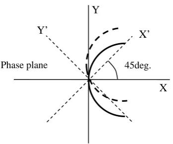
From the experience dealing with extensive subsurface models, it is not likely to observe the orbit of characteristic function approaching and leaving the origin with acute angel less than 90 degree in the phase plane. Then we propose two-dimensional zero-cross root finding algorithm as shown in Fig. 3, where either simultaneous sign change of the real part and the imaginary part or simultaneous sign change of them with reference to 45 degree rotated axes in the phase plane can be used to identify complex number zero-crossing. This approach can deal with rotated and distorted Rayleigh wave’s orbit, as well as regular Love wave’s orbit without watching real value of characteristic functions. It is noted that the bisection algorithm cannot distinguish real zero-cross and sign changed divergence at a singular point, so that we have to verify reduction of absolute value of relevant entities for the two-dimensional bisection algorithm across the possible zero-cross point.
Since characteristic function contains sign-varying radicals related to S wave velocity and P wave velocity of the layers, it may be advantageous to divide the characteristic function by the products of radicals related to the body wave velocities as shown in Hisada (1997) to make the evaluation of the characteristic function easier.
4.2 Bisection algorithm down along frequency axis
If we have to evaluate segmentation necessary for the bisection method along velocity axis at each frequency, sign change should be evaluated inch by inch repeatedly from the possible lowest velocity to the possible highest velocity. Since we know that number of roots decreases at lower frequencies, and dispersion curves are continuous with adequate smoothness along frequency axis, we can utilize prior information at higher frequencies to set segmentation at lower frequencies by assuming densely populated frequency steps as shown in Fig. 4. We set end points of an initial segment at a frequency in between the roots evaluated at the prior higher frequency to increase efficiency of the bisection method.
Fig.3 Scheme for finding zero-cross of complex characteristic function:
An orbit expressed by thick line zero-crosses X axis while leaving X value evaluation necessary near the origin. But, for the orbit zero-crosses both of X’ and Y’ axes, rotated from X-Y system by 45 degree, value assurance with threshold is not necessary.
45deg.
X X’ Y
Y’
5. EXAMPLES AND DISCUSSIONS 5.1 Example models
We will examine how the root finding algorithm works with several representative examples. We use two example structures for two layers underlain by semi-infinite space; Model-1 with increasing S wave velocity
with depth as shown in Table 2, and Model-2 with weak 2nd layer of less S wave velocity sandwiched between
the top layer and half-space as shown in Table 3. For more realistic subsurface model, we use multi-layered model shown in Table 4 with thick internal layer of less S wave velocity. In these examples, we have computed dispersion curves only for several modes without relying on the root tracking algorithm along frequency axis; we have made 2000 trial search for bisection segmentation between 80 % of the minimum S wave velocity to the maximum velocity at each frequency.
5.2 Love waves
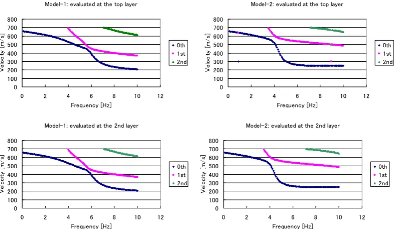
For the two-layered models, we can evaluate Love wave dispersion curves for the fundamental and the 1st
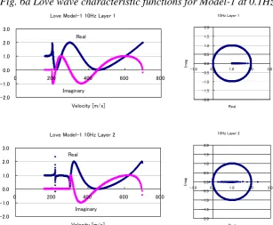
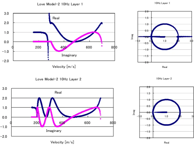
modes up to 10 Hz shown in Fig. 5 by the aforementioned root finding algorithm. Characteristic functions for these models have basically a clockwise circular orbit at 0.1Hz and 10Hz irrespective of models and layers as shown in Fig. 6 and Fig. 7. Although we cannot distinguish dispersion curves between characteristic functions evaluated at different layers, the orbit for the layer with smaller S wave velocity, layer 1 for the model-1 and layer 2 for the model-2, is confined to the inside of a unit circle without showing sudden change compared to the one for the other layer, which may be preferable for finding roots.
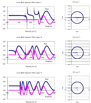
For multi-layered subsurface model with weak layer inclusion, dispersion curves shown in Fig. 8 are obtained by the root finding algorithm applied to characteristic functions evaluated at different layers. We can evaluate smooth dispersion curves with the fifth layer, but worse result at higher frequencies with the second layer, and the worst result with the top layer of the three. The characteristic functions at 12 Hz are shown in Fig. 9 for the top layer, the second layer of the smallest S wave velocity, and the fifth layer of relatively small S wave velocity, where circular orbits are commonly drawn for these layers. However, linear parts lay inside the unit circles for layers with less S wave velocity, such as the second layer and the fifth layer, with less sudden change along velocity axis, enabling more stable evaluation for dispersion curves.
These examples and other experiences make us conclude empirically that Love wave characteristic function draws linear horizontal plus unit circular orbits in the phase plane in general. Characteristic functions show less diverging fluctuations for layers with smaller S waves, leading to better evaluation of dispersion curves.
5.3 Rayleigh waves
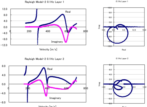
For the model-1, we can evaluate Rayleigh wave dispersion curves for the first three modes up to 10 Hz shown in Fig. 10 with different layer of evaluation, and there are some frequencies where we cannot evaluate Rayleigh wave velocity for the model-2. Characteristic functions show rotated and distorted circle with linear horizontal orbits along the velocity axis at 0.1Hz and 10Hz irrespective of models and layers as shown in Fig. 11 and Fig. 12 without showing any linear orbit confined in a distorted circle unlike the case of Love waves.
Fig.4 Root tracking algorithm along frequency axis
FhFl Velocity upper Bound
Velocity lowe Bound
zero-cross search segment
Characteristic function evaluated at a layer of less S wave velocity tends to show less singular fluctuation leading to more stable evaluation of dispersion curves as was the case in Love waves.
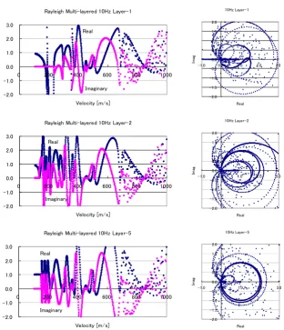
For the multi-layered model, advantage of evaluation at a softer layer seen in Love waves is more pronounced. We can get satisfactory dispersion curves for the first four modes with the fifth layer from 1 Hz to 12 Hz, but it is worse for the second layer at high frequencies and getting worse for the top layer as shown in Fig. 13. The characteristic functions for the layers at 1 Hz and 10 Hz are shown in Fig. 14 revealing more regular orbit and less singular oscillation at 10 Hz for the fifth layer compared to the other layers while retaining similar fluctuation at 1 Hz to them.
5.4 Discussions
We have examined behaviors of characteristic functions derived by generalized TR matrices for Love and Rayleigh waves in the phase plane to propose the two-dimensional bisection method for finding roots of zero-crossing with efficient segmentation search down along frequency axis utilizing roots found for prior higher frequency. Applying the two-dimensional bisection method to two-layered and multi-layered example subsurface structures, it is found that orbits are made up of lines along real axis and unit circles for Love waves irrespective of layer of evaluation, frequency, and structure. For Rayleigh waves, they are made up of lines along real axis and rotated and distorted circles. With these examples, it is not advisable to use the top layer unconditionally for dispersion curve evaluation; rather evaluation of characteristic functions at an adequately thick layer with less S wave velocity is empirically advisable. This is a classic problem with tremendous number of literatures, but still draws an attention in conjunction with on-site surface wave inversion of recent trends using micro-tremor observation.
Table 2. Two-layered model with increasing S wave velocity with depth
Depth to bottom [m] Density [g/cm3] S wave velocity [m/s] P wave velocity [m/s]
10.0 2.0 200. 400 20.0 2.0 300. 800 Infinite 2.0 700. 1600
Table 3. Two-layered model with less S wave velocity layer penetrated
Depth to bottom [m] Density [g/cm3] S wave velocity [m/s] P wave velocity [m/s]
10.0 2.0 300. 800 20.0 2.0 200. 400 Infinite 2.0 700. 1600
Table 4. Multi-layered subsurface model
Depth to bottom [m] Density [g/cm3] S wave velocity [m/s] P wave velocity [m/s]
Model-1
0 100 200 300 400 500 600 700 800
0 2 4 6 8 10 12
Frequency [Hz]
V
e
lo
c
it
y
[m/
s]
0th 1st
Model-2
0 100 200 300 400 500 600 700 800
0 2 4 6 8 10 12
Frequency [Hz]
V
e
lo
c
it
y
[m/
s]
0th 1st
Fig. 5 Love wave dispersion curves for two-layered models
Love Model-1 0.1Hz Layer 1
-2.0 -1.0 0.0 1.0 2.0 3.0
0 200 400 600 800
Velocity [m/s] Real
Imaginary
0.1Hz Layer 1
-2.0 -1.5 -1.0 -0.5 0.0 0.5 1.0 1.5 2.0
-1.0 0.0 1.0 2.0 3.0
Real
Im
ag
Love Model-1 0.1Hz Layer 2
-2.0 -1.0 0.0 1.0 2.0 3.0
0 200 400 600 800
Velocity [m/s] Real
Imaginary
0.1Hz Layer 2
-2.0 -1.5 -1.0 -0.5 0.0 0.5 1.0 1.5 2.0
-1.0 0.0 1.0 2.0 3.0
Real
Im
ag
Fig. 6a Love wave characteristic functions for Model-1 at 0.1Hz
Love Model-1 10Hz Layer 1-2.0 -1.0 0.0 1.0 2.0 3.0
0 200 400 600 800
Velocity [m/s] Real
Imaginary
10Hz Layer 1
-2.0 -1.5 -1.0 -0.5 0.0 0.5 1.0 1.5 2.0
-1.0 0.0 1.0 2.0 3.0
Real
Im
ag
Love Model-1 10Hz Layer 2
-2.0 -1.0 0.0 1.0 2.0 3.0
0 200 400 600 800
Velocity [m/s] Real
Imaginary
10Hz Layer 2
-2.0 -1.5 -1.0 -0.5 0.0 0.5 1.0 1.5 2.0
-1.0 0.0 1.0 2.0 3.0
Real
Im
ag
Love Model-2 0.1Hz Layer 1
-2.0 -1.0 0.0 1.0 2.0 3.0
0 200 400 600 800
Velocity [m/s]
Real
Imaginary
0.1Hz Layer 1
-2.0 -1.5 -1.0 -0.5 0.0 0.5 1.0 1.5 2.0
-1.0 0.0 1.0 2.0 3.0
Real
Im
ag
Love Model-2 0.1Hz Layer 2
-2.0 -1.0 0.0 1.0 2.0 3.0
0 200 400 600 800
Velocity [m/s]
Real
Imaginary
0.1Hz Layer 2
-2.0 -1.5 -1.0 -0.5 0.0 0.5 1.0 1.5 2.0
-1.0 0.0 1.0 2.0 3.0
Real
Im
ag
Fig. 7a Love wave characteristic functions for Model-2 at 0.1Hz
Love Model-2 10Hz Layer 1
-2.0 -1.0 0.0 1.0 2.0 3.0
0 200 400 600 800
Velocity [m/s] Real
Imaginary
10Hz Layer 1
-2.0 -1.5 -1.0 -0.5 0.0 0.5 1.0 1.5 2.0
-1.0 0.0 1.0 2.0 3.0
Real
Im
ag
Love Model-2 10Hz Layer 2
-2.0 -1.0 0.0 1.0 2.0 3.0
0 200 400 600 800
Velocity [m/s] Real
Imaginary
10Hz Layer 2
-2.0 -1.5 -1.0 -0.5 0.0 0.5 1.0 1.5 2.0
-1.0 0.0 1.0 2.0 3.0
Real
Im
ag
Multi-layer: evaluated at Layer 1
0 200 400 600 800 1000
0 2 4 6 8 10 12
Frequency [Hz]
V
e
lo
c
it
y
[m/
s]
0th 1st 2nd 3rd
Multi-layer: evaluated at Layer 2
0 200 400 600 800 1000
0 2 4 6 8 10 12
Frequency [Hz]
V
e
lo
c
it
y
[m/
s]
0th 1st 2nd 3rd
Multi-layer: evaluated at Layer 5
0 200 400 600 800 1000
0 2 4 6 8 10 12
Frequency [Hz]
V
e
lo
c
it
y
[m/
s]
0th 1st 2nd 3rd
Fig. 8 Love wave dispersion curves for a multi-layered model
Love Multi-layered 12Hz Layer-1
-2.0 -1.0 0.0 1.0 2.0 3.0
100 150 200 250 300
Velocity [m/s]
Real
Imaginary
12Hz Layer-1
-2.0 -1.5 -1.0 -0.5 0.0 0.5 1.0 1.5 2.0
-1.0 0.0 1.0 2.0 3.0
Real
Im
ag
s
Love Multi-layered 12Hz Layer-2
-2.0 -1.0 0.0 1.0 2.0 3.0
100 150 200 250 300
Velocity [m/s]
Real
Imaginary
12Hz Layer-2
-2.0 -1.5 -1.0 -0.5 0.0 0.5 1.0 1.5 2.0
-1.0 0.0 1.0 2.0 3.0
Real
Im
ag
Love Multi-layered 12Hz Layer-5
-2.0 -1.0 0.0 1.0 2.0 3.0
100 150 200 250 300
Velocity [m/s]
Real
Imaginary
12Hz Layer-5
-2.0 -1.5 -1.0 -0.5 0.0 0.5 1.0 1.5 2.0
-1.0 0.0 1.0 2.0 3.0
Real
Im
ag
Model-1: evaluated at the top layer
0 100 200 300 400 500 600 700 800
0 2 4 6 8 10 12
Frequency [Hz]
V
e
lo
c
it
y
[m/
s]
0th 1st 2nd
Model-2: evaluated at the top layer
0 100 200 300 400 500 600 700 800
0 2 4 6 8 10 12
Frequency [Hz]
V
e
lo
c
it
y
[m/
s]
0th 1st 2nd
Model-1: evaluated at the 2nd layer
0 100 200 300 400 500 600 700 800
0 2 4 6 8 10 12
Frequency [Hz]
Ve
loc
it
y [
m
/
s]
0th 1st 2nd
Model-2: evaluated at the 2nd layer
0 100 200 300 400 500 600 700 800
0 2 4 6 8 10 12
Frequency [Hz]
Ve
loc
it
y [
m
/
s]
0th 1st 2nd
Fig. 10 Rayleigh wave dispersion curves for two-layered models
Rayleigh Model-1 0.1Hz Layer 1
-8.0 -4.0 0.0 4.0 8.0
0 200 400 600 800
Velocity [m/s] Real
Imaginary
0.1Hz Layer 1
-8.0 -6.0 -4.0 -2.0 0.0 2.0 4.0 6.0 8.0
-4.0 0.0 4.0 8.0 12.0
Real
Im
ag
Rayleigh Model-1 0.1Hz Layer 2
-12.0 -8.0 -4.0 0.0 4.0 8.0 12.0
0 200 400 600 800
Velocity [m/s] Real
Imaginary
0.1Hz Layer 2
-12.0 -9.0 -6.0 -3.0 0.0 3.0 6.0 9.0 12.0
-6.0 0.0 6.0 12.0 18.0
Real
Im
ag
Rayleigh Model-1 10Hz Layer 1
-4.0 -2.0 0.0 2.0 4.0
0 200 400 600 800
Velocity [m/s] Real
Imaginary
10Hz Layer 1
-4.0 -3.0 -2.0 -1.0 0.0 1.0 2.0 3.0 4.0
-2.0 0.0 2.0 4.0 6.0
Real
Im
ag
Rayleigh Model-1 10Hz Layer 2
-4.0 -2.0 0.0 2.0 4.0
0 200 400 600 800
Velocity [m/s] Real
Imaginary
10Hz Layer 2
-4.0 -3.0 -2.0 -1.0 0.0 1.0 2.0 3.0 4.0
-2.0 0.0 2.0 4.0 6.0
Real
Im
ag
Fig. 11b Rayleigh wave characteristic functions for Model-1 at10Hz
Rayleigh Model-2 0.1Hz Layer 1
-12.0 -8.0 -4.0 0.0 4.0 8.0 12.0
0 200 400 600 800
Velocity [m/s] Real
Imaginary
0.1Hz Layer 1
-12.0 -9.0 -6.0 -3.0 0.0 3.0 6.0 9.0 12.0
-6.0 0.0 6.0 12.0 18.0
Real
Im
ag
Rayleigh Model-2 0.1Hz Layer 2
-8.0 -4.0 0.0 4.0 8.0
0 200 400 600 800
Velocity [m/s] Real
Imaginary
0.1Hz Layer 2
-8.0 -6.0 -4.0 -2.0 0.0 2.0 4.0 6.0 8.0
-4.0 0.0 4.0 8.0 12.0
Real
Im
ag
Rayleigh Model-2 10Hz Layer 1
-8.0 -6.0 -4.0 -2.0 0.0 2.0 4.0 6.0 8.0
0 200 400 600 800
Velocity [m/s] Real
Imaginary
10Hz Layer 1
-8.0 -6.0 -4.0 -2.0 0.0 2.0 4.0 6.0 8.0
-4.0 0.0 4.0 8.0 12.0
Real
Im
ag
Rayleigh Model-2 10Hz Layer 2
-4.0 -3.0 -2.0 -1.0 0.0 1.0 2.0 3.0 4.0
0 200 400 600 800
Velocity [m/s] Real
Imaginary
10Hz Layer 2
-4.0 -3.0 -2.0 -1.0 0.0 1.0 2.0 3.0 4.0
-2.0 0.0 2.0 4.0 6.0
Real
Im
ag
Fig. 12b Rayleigh wave characteristic functions for Model-2 at 10Hz
Multi-layer: evaluated at Layer 1
0 200 400 600 800 1000
0 2 4 6 8 10 12
Frequency [Hz]
Vel
o
ci
ty
[
m
/
s]
0th 1st 2nd 3rd
Multi-layer: evaluated at Layer 2
0 200 400 600 800 1000
0 2 4 6 8 10 12
Frequency [Hz]
Ve
loc
it
y [
m
/
s]
0th 1st 2nd 3rd
Multi-layer: evaluated at Layer 5
0 200 400 600 800 1000
0 2 4 6 8 10 12
Frequency [Hz]
Vel
o
ci
ty
[
m
/
s]
0th 1st 2nd 3rd
Rayleigh Multi-layered 1Hz Layer-1
-2.0 -1.0 0.0 1.0 2.0 3.0
0 200 400 600 800 1000
Velocity [m/s] Real
Imaginary
1Hz Layer-1
-2.0 -1.5 -1.0 -0.5 0.0 0.5 1.0 1.5 2.0
-1.0 0.0 1.0 2.0 3.0
Real
Im
ag
s
Rayleigh Multi-layered 1Hz Layer-2
-2.0 -1.0 0.0 1.0 2.0 3.0
0 200 400 600 800 1000
Velocity [m/s] Real
Imaginary
1Hz Layer-2
-2.0 -1.5 -1.0 -0.5 0.0 0.5 1.0 1.5 2.0
-1.0 0.0 1.0 2.0 3.0
Real
Im
ag
s
Rayleigh Multi-layered 1Hz Layer-5
-2.0 -1.0 0.0 1.0 2.0 3.0
0 200 400 600 800 1000
Velocity [m/s] Real
Imaginary
1Hz Layer-5
-2.0 -1.5 -1.0 -0.5 0.0 0.5 1.0 1.5 2.0
-1.0 0.0 1.0 2.0 3.0
Real
Im
ag
s
Rayleigh Multi-layered 10Hz Layer-1
-2.0 -1.0 0.0 1.0 2.0 3.0
0 200 400 600 800 1000
Velocity [m/s] Real
Imaginary
10Hz Layer-1
-2.0 -1.5 -1.0 -0.5 0.0 0.5 1.0 1.5 2.0
-1.0 0.0 1.0 2.0 3.0
Real
Im
ag
s
Rayleigh Multi-layered 10Hz Layer-2
-2.0 -1.0 0.0 1.0 2.0 3.0
0 200 400 600 800 1000
Velocity [m/s] Real
Imaginary
10Hz Layer-2
-2.0 -1.5 -1.0 -0.5 0.0 0.5 1.0 1.5 2.0
-1.0 0.0 1.0 2.0 3.0
Real
Im
ag
s
Rayleigh Multi-layered 10Hz Layer-5
-2.0 -1.0 0.0 1.0 2.0 3.0
0 200 400 600 800 1000
Velocity [m/s] Real
Imaginary
10Hz Layer-5
-2.0 -1.5 -1.0 -0.5 0.0 0.5 1.0 1.5 2.0
-1.0 0.0 1.0 2.0 3.0
Real
Im
ag
s
Fig. 14b Rayleigh wave characteristic functions for a multi-layered model at 10Hz
REFERENCES
Chen, X., (1993), A systematic and efficient method of computing normal modes for multilayered half-space, Geophys. J. Int., Vol. 115, pp. 391-409.
Haskell, N. A., (1953), The dispersion of surface waves on multilayered media, Bull. Seism. Soc. Am., Vol. 43, pp. 17-34.
Hisada, Y., (1997), Efficient methods for computing Green’s functions and normal mode solutions for layered half-spaces, J. Struct. Constr. Eng., AIJ, No. 501, pp. 49-56, in Japanese.
Luco, J. E. and R. J.Apsel, (1983), On the Green’s functions for a layered half-space, Part 1, Bull. Seism. Soc. Am., Vol. 73, No. 4, pp. 909-929.
Press, W. H., S. A. Teukolsky, W T.Vetterling, and B. P. Flannery, (2003), Numerical recipes in C++, Cambridge University Press.
![Table 1. Multilayered crustal model (Chen, 1993) Density [g/cm3] S wave velocity [km/s]](https://thumb-us.123doks.com/thumbv2/123dok_us/1738248.1222347/3.595.64.531.600.664/table-multilayered-crustal-model-chen-density-wave-velocity.webp)
![Table 4. Multi-layered subsurface model S wave velocity [m/s] 233](https://thumb-us.123doks.com/thumbv2/123dok_us/1738248.1222347/7.595.65.531.536.717/table-multi-layered-subsurface-model-s-wave-velocity.webp)