Semiparametric Inference Based on a Class of
Zero-Altered Distributions
Sujit K. Ghosh and Honggie Kim
Department of Statistics, NC State University.
Institute of Statistics Mimeo Series #2589
Abstract
In modeling count data collected from manufacturing processes,
eco-nomic series, disease outbreaks and ecological surveys, there are usually
a relatively large or small number of zeros compared to positive counts.
Such low or high frequencies of zero counts often require the use of
un-der or over dispersed probability models for the unun-derlying data generating
mechanism. The commonly used models such as generalized or zero-inflated
Poisson distributions can usually account for only the over dispersion, but
such distributions are often found to be inadequate in modeling
underdis-persion because of the need for awkward parameter or support restrictions.
This article introduces a flexible class of semiparametric zero-altered models
which account for both under and over dispersion and includes other
famil-iar models such as those mentioned above as special cases. Consistency and
asymptotic normality of the dispersion parameter are derived under general
conditions. Numerical support for the performance of the proposed method
of inference is presented for the case of common discrete distributions.
Keywords: Asymptotic normality; Consistency; Overdispersion; Semiparametric
1
Introduction
Statistical methods for analyzing count data with too few or too many zeros are
very important in various scientific fields including but not limited to industrial
applications (e.g., Lambert, 1992), econometrics (e.g., Cameron and Trivedi, 1986)
and biomedical applications (e.g., Heilbron and Gibson, 1990, Hall, 2000). Most
of these applications were motivated by the observed overdispersion due to excess
zero counts. For other interesting applications related to zero-inflated models see
Dahiya and Gross (1973), Umbach (1981), Yip (1988), Gupta et al. (1996), Welsh
et al. (1996), Gurmu (1997) and Hinde and Demetrio (1998). An overview of zero
inflated models can be found in Ridout et al. (1998) and Tu (2002). However
underdispersion can also be observed in practice (Famoye, 1993). As the case of
underdispersion is relatively rare (but not inevitable) we present a data set that
features underdispersion (see Table 1). Winkelmann and Zimmermann (1995)
present many illustrations and applications. From their article we quote only a
few areas of potential applications: the analysis of accident proneness (e.g., airline
failures), labor mobility (the number of changes of employer), the demand for
health-care services (as measured by the number of doctor consultations in a given
time) and, in economic demography, total fertility (the number of births by a
woman). Winkelmann and Zimmermann (1995) also provides a thorough review
of related statistical inference for count data, mostly based on parametric models.
Our proposed model includes most of such parametric models as special cases
within a semiparametric framework.
As an illustration, consider the data set in Table 1 that aims modeling the
func-tion word counts (Bailey, 1990). The data show clear evidence of underdispersion.
There are several other data sets as above which show evidence of
underdisper-sion. We use the above mentioned data set as a motivating example to develop our
models for count data with relatively low or high proportion of zeros. However, by
In this article, we propose a new class of zero-altered distributions that can
account for both under and over dispersion. This is similar in spirit to the work of
Castillo and Perez-Casany (2005) who have recently introduced a class of
paramet-ric generalizations of the Poisson distribution that can also account for both under
and over dispersion. However we find the class of such weighted version of Poisson
distributions (see Rao, 1965) to be somewhat inflexible in practice. For instance,
closed form analytical expressions for the normalizing constants are not available
in general, which leads to only implicit function representation of the moments of
the distribution. Further only an approximate log-linear models can be used to fit
such distributions as the closed form of the likelihood is not available. Although
their models seem to include the class zero-modified distributions (Johnson et al.,
1992), but in order to capture underdispersion the weighting parameter needs to
be truncated by a bound that will depend on other parameters (e.g., in equation
(4) of Castillo and Perez-Casany (2005), one requires > −p0/(1−p0), where p0 is probability of a zero count under a parametric model, such as Poisson model).
We propose a class of semiparametric models that avoids the above mentioned
analytical and practical limitations.
We show that besides the flexibility of modeling both types of dispersion, the
proposed distributions have several other advantages: (i) the support of the
distri-butions is N = {0,1,2, . . .} even when the distribution is underdispersed; (ii) the
parameter value (which we denote by δ) that determines the nature of dispersion
lies in the open interval (e.g. δ ∈ (−1,1)); (iii) asymptotic distributions of the
estimator ˆδ and the test statistic under the null hypothesis H0 :δ = 0, both have normal distributions; and last but not the least (iv) the estimation methodology
is based on a semiparametric model. It may be noted that absolute bounds of
the parameter δ ∈ (−1,1) makes it easier to formulate regression problems using
suitable link functions.
1994) with no assumption on the underlying equidispersed distribution. Section 3
presents statistical inference based on an M-estimation theory. Section 4 illustrates
the procedure with real-life data sets presented at the beginning of this section and
also presents results based on simulation studies. Section 5 concludes this study
and addresses a few areas of future research.
2
Generalized Zero-Altered Distributions
Consider a non-degenerate random variable U taking values in N = {0,1,2, . . .}
with probability mass functionf0(u) foru∈N, i.e.,f0(u)≥0 and∞u=0f0(u) = 1. Without loss of any generality we assume that f0(0)<1. We can modify any such probability mass function by altering its probability at u = 0, using a dispersion
parameter, δ ∈ (−1,1) by defining a new class of probability mass functions as
follows:
fδ(x) =
⎧ ⎨ ⎩
δ2
++ (1−δ2)f0(0) if x= 0
1−δ+2 +δ−21−f0f(0) 0(0)
f0(x) for x= 1,2, . . .
(1)
Here, we have used the standard notations, δ+= max{δ,0} and δ−= max{−δ,0} to denote the positive and negative part of δ, so thatδ=δ+−δ−. Clearly, for any
|δ|<1, the function fδ(·) in (1) is a probability mass function (pmf). Also notice
that, fδ=0 = f0, so that f0 is included in the class of distributions generated by
fδ(·). Notice that in (1) instead ofδ+2 we could have usedδ+ or more generally any
smooth increasing function ofδ+. However our choice makesfδ a smooth function
of δ having a continuous first derivative with respect to δ, which will turn out to
be useful in deriving the asymptotic inference (see Section 3).
In order to study the general properties of fδ, let X denote a statistic with
probability mass function fδ, which we will denote byX ∼ fδ, δ ∈(−1,1). First,
notice that the representation in (1) is unique in the sense that if there were δ∗ and f0∗, such thatfδ(·) = fδ∗(·) and f0(0)−f0∗(0), then δ =δ∗ and f0(·) = f0∗(·).
restriction on f0(·) (e.g., f0(0) = 0.5 etc.). Next we show that fδ can account for
both over and under dispersion.
Definition 1. A random variable X having finite second moment is said to
be underdispersed or overdispersed if μ > σ2 or μ < σ2, respectively, where μ=E[X] and σ2 =V ar[X] denote the mean and variance of the random variable X, respectively. If X is neither under nor over dispersed, i.e., if μ =σ2, then X is said to be equidispersed.
From here on, we assume that Ef0[U2] < ∞, i.e., ∞u=1u2f0(u) < ∞. It
immediately follows from (1) that if X ∼ fδ then E[X2] <∞ for all δ ∈ (−1,1).
We now state the mean and variance of X ∼fδ in terms of the mean μ0 =Ef0[U]
and variance σ02 =V arf0[U] of the underlying random variableU.
Lemma 1. The mean μ and the variance σ2 of X ∼fδ is given by
μ = ω(δ)μ0 (2)
σ2 = ω(δ)σ2 0 +
1−ω(δ)
ω(δ) μ
2, (3)
where ω(δ) =
1−δ+2 +δ−2 f0(0)
1−f0(0)
.
Lemma 1 easily follows from the fact that fδ(x) = ω(δ)f0(x) for x= 0, which
in turn implies that E[X] = ω(δ)E[U] = ω(δ)μ0 and E[X2] = ω(δ)E[U2] =
ω(δ)(σ20 +μ20). Based on Lemma 1 we can derive the following result:
Theorem 1. Suppose X ∼ fδ, where fδ is given by (1) and assume that the
underlying random variable U is equidispersed, i.e., μ0 =σ02. Then X is
underdispersed i.e., μ > σ2 if δ <0,
equidispersed i.e., μ=σ2 if δ= 0,
Proof: From (3) of Lemma 1 it follows that whenU is equidispersed (i.e.,μ0 =σ02),
σ2−μ= 1−ω(δ)
ω(δ) μ2 and
1−ω(δ)
ω(δ) = ⎧ ⎨ ⎩
1−δ2
δ2 if δ >0
−δ2f0(0)
1−(1−δ2)f0(0) if δ ≤0.
Thus, σ2−μ has the same sign as δ. This completes the proof of Theorem 1.
The above result clearly indicates thatδacts as a measure of dispersion; a
nega-tive value (δ <0) indicates underdispersion while a positive value (δ >0) indicates
overdispersion and a value of zero (δ = 0) indicates equidispersion. Theorem 1 can
be generalized when the underlying random variable U is not equidispersed, but
then we can always obtain under and over dispersed models using the modification
in (1). In this sense, we can restrict the underlying distribution to belong to a class
of equidispersed distributions (e.g., a Possion distribution). Appendix A presents
an extension of Theorem 1, when U is not necessarily equidispersed.
In general, any discrete distribution could be used for U, however to derive
asymptotic inference and parsimony we restrict our attention to only an
equidis-persed discrete distribution for U. Moreover, given any random variable X with
pmf g(·) and having a finite second moment, we can find δ and f0(·) such that
fδ(·) =g(·), wheref0(·) satisfiesμ0 =σ20 (see Theorem 4 in the Appendix). Based
on this semiparametric model for X we develop estimation and testing
method-ology based on the general theory of M-estimation (Boos and Stefanski, 2002)
methods.
3
Statistical Inference
Let X1, . . . , Xn be a independent and identically distributed (iid) random
vari-ables with common distribution fδ(x) as given in (1) with the restriction that
∞
distribution for U is assumed other than the fact that U is equidispersed. Let
π0 =f0(0) andω(δ, π0) = 1−δ+2 +δ−2 π0
1−π0. Under the above assumption, it follows thatE[X] =μ0ω(δ, π0), E[X(X−1)] =μ20ω(δ, π0) and Pr[X = 0] =δ2++(1−δ2)π0. The above three facts lead to the following set of estimating equations:
n
i=1
ψ1(Xi,θ) = n
i=1
(Xi−θ3ω(θ1, θ2)) = 0 n
i=1
ψ2(Xi,θ) = n
i=1
(Xi(Xi−1)−θ32ω(θ1, θ2)) = 0 and (4) n
i=1
ψ1(Xi,θ) = n
i=1
(I{0}(Xi)−θ21+−(1−θ12)θ2) = 0
whereIA(x) denotes the indicator function such thatIA(x) = 1 ifx∈A, otherwise
IA(x) = 0 and θ = (θ1, θ2, θ3) whereθ1 =δ, θ2 =π0 and θ3 =μ0
From here on we assume that there is aθ0 ∈Θ = (−1,1)×(0,1)×(0,∞) such
that Eθ
0[ψ(θ, X)] = 0 if and only if θ = θ0, where Eθ0 denotes the expectation with respect to f(x|θ0) andψ(·,·) = (ψ1(·,·), ψ2(·,·), ψ3(·,·)). In other words, the true pmf of the data is given by f(x|θ0) (as defined in (1)) for some θ0 ∈ Θ.
Notice that as the underlying pmf f0 of U is specified only up to second moment, any pmf with finite second moment belongs to the class of our proposed models
M = {f(x|θ) : θ ∈ Θ} (see Theorem 4 in the Appendix). We now develop an estimator of θ0 (and in particular θ10 =δ0) that is consistent and asymptotically normal for the model M.
Let ¯X = ni=1Xi/n and S2 = ni=1(Xi −X¯)2/(n − 1) denote the sample
mean and sample variance, respectively. Also let P0 = ni=1I{0}(Xi)/n denotes
the proportion of zeros observed in the sample. It follows easily that the equation
(4) is equivalent to solving:
¯
X = θ3ω(θ1, θ2),
n−1
Now, by solving (5) we obtain,
ˆ
δ= ˆθ1 = sgn(D) |D|
|D|+RX¯2,
ˆ
π0 = ˆθ2 = (P0 ¯
X2−D(1−P 0))
¯
X2 and (6)
ˆ
μ0 = ˆθ3 = (D+ ¯X
2)
¯
X ,
where D = n−n1S2 −X¯ and R = P0/(1−P0) if D < 0 and R = 1 otherwise. As expected, it follows from (6) that the sign of ˆδ is determined by the sign of D
denoted by sgn(D).
We can use the above estimator ˆδ as a test statistic to test the null hypothesis
H0 :δ= 0 against two-sided or one-sided alternatives. Also we may obtain a con-fidence interval for δ by deriving the standard error (s.e.) of ˆδ. As the form of the
ˆ
δ is complicated, we have at least two options: (a) obtain a bootstrap distribution
of ˆδ (Efron and Tibshirani, 1993) or (b) obtain the asymptotic distribution of ˆδ
using the M-estimation formulation as given in (4). Although our main interest
is in estimating the dispersion parameter δ, by solving (5) (or equivalently (4)),
we have also obtained the estimates of μ0 and π0 (as given in 6)). We can use (nonparametric) bootstrap to make inference about these underlying (nuisance)
parameters as well.
Clearly ψ(·, x) is a smooth function of θ having a continuous first derivative
and also ψ(θ,·) is a Borel measurable function for allθ ∈ Θ, where Θ is an open
set as defined above. Thus, it follows that the regularity conditions needed to
derive the asymptotic distribution of ˆθ (given by Huber, 1967) are satisfied in this
case.
We now derive the so-called “A =A(θ) matrix” and the “B = B(θ) matrix”
asymp-totic variance, V =V(θ) = A−1B(A−1)T, where
A(θ) = −Eθ[∇θψ(θ, X)]
B(θ) = Eθ[ψ(θ, X)ψ(θ, X)T]
where∇θψ(θ, x) denotes gradient ofψ(θ, x) with respect toθ. Notice thatψ(θ, x)
is of the form a(x) +b(θ) for some functions a(·) and b(·) and hence we do not
have to compute the expected value of∇θψ(θ, x) to obtain the “A-matrix”. Since
ψ2(θ, x) = x(x−1)−θ3ω(θ1, θ2) it follows that in order to haveB(θ) finite we need to assume that X has finite fourth moment, i.e., we assume Eθ
0[X
4] <∞ which
in turn is equivalent to the assumption that E[U4]<∞. Notice that we need this latter assumption only for the asymptotic normality; the estimator ˆθ is consistent
even when the forth moment is not finite. We now state the main theorem that
provides the consistency and asymptotic normality of the estimator ˆθ:
Theorem 2. Suppose X1, . . . , Xn are iid f(x|θ) where f(·|·) is given by (1)
with θ1 = δ, θ2 = π0 and θ3 = μ0. Assume that σ02 < ∞ and μ0 = σ20. Then the M-estimator ˆθ given by (6) is uniformly consistent.
Further, if E[U4] <∞, then θˆ converges in distribution to a normal distribu-tion. More precisely,
√
n(ˆθ−θ0)→N(0, V(θ0)), (7)
where V(θ0) =A(θ0)−1B(θ0)(A(θ0)−1)T
Proof: It easily follows that ψ(θ, x) satisfies all the regularity conditions
(B-1)-B(4) of Theorem 2 in Huber (1967) and hence the consistency follows from the
general theory of M-estimation.
For asymptotic normality it is possible to show that the regularity conditions
(N-1)-(N-4) of Theorem 3 in Huber (1967) are satisfied and hence by the corollary
to the Theorem 3 in Huber (1967) the result follows. Some technical details are
We now derive the exact form of the “A-matrix”. Letaij = ∂ψ∂θji(θ, x). As noted
earlier aij’s do not depend on x and hence A(θ) = ((aij(θ)))3×3. It easily follows
that,
a11 = −θ3∂ω
∂θ1 = 2θ3
θ1++θ1− θ2 1−θ2
,
a12 = −θ3∂ω
∂θ2 =−θ3
θ
1−
1−θ2
2
,
a13 = −ω(θ1, θ2),
a21 = θ3a11, a22=θ3a12, a23= 2θ3a13
a31 = −2(θ1+−θ1θ2), a32=−(1−θ1−)2 and a33= 0
The closed of expression for the “B-matrix” can also be derived similarly involving
up to the forth moments of U. If the distribution of U is specified parametrically
(e.g., U ∼P oisson(λ)), then we can easily obtain a closed form expression for the
“B-matrix” similar to the closed form expression of “A-matrix” as given above.
However it turns out that for estimation (and to obtain confidence interval), we
can estimate the A and B matrices using the following consistent estimators:
ˆ
A=A(ˆθ) = ((aij(ˆθ)))
ˆ
B = ˆB(ˆθ) = 1
n
n
i=1
ψ(ˆθ, Xi)ψ(ˆθ, Xi)T
and hence we can obtain ˆV = ˆA−1Bˆ( ˆA−1)T to obtain the standard errors of ˆθ. As ˆV is a consistent estimator ofV(θ0) (see Iverson and Randles, 1989) it follows
from Theorem 2 (by an use of the Slutsky’s Theorem) that √nVˆ−1/2(ˆθ − θ0) converges in distribution to a trivariate normal distribution with mean vector zero
and variance covariance matrix an identity matrix of order 3. Hence, it follows
that, √n(ˆδ−δ0)∼AN(0,e1TVˆe1) wheree1 = (1,0,0)T.
Alternatively, as the forth moment condition can not be checked in general, we
may prefer the use of the bootstrap method (Efron and Tibshirani, 1993) to make
occurrences 5-word count 10-word count
0 45 27
1 49 44
2 6 26
>2 0 3
¯
x 0.61 1.05
s2 0.36 0.65
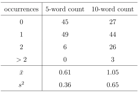
Table 1: Frequency of function word counts.
apply these results to a data set and study the performance of the method using
a simulation study motivated by the real data application.
4
Simulation and Data Analysis
In this section, first we analyze the data listed in Table 1 to illustrate the methods
described in Section 3. In addition to the asymptotic s.e. of the estimator ˆδwe also
compute a bootstrap distribution of ˆδand compare its value to the asymptotic s.e.
obtained by the M-estimation theory. We conclude this section with a simulation
study motivated by this real application to see the performance of the proposed
estimates.
4.1
Application to function word count data
First, we analyze the data presented in Table 1 which presents a count of function
words for n = 100 words. In studies aimed at characterizing an author’s style,
samples of m words are taken and the number of function words in each sample
counted. Often binomial or Poisson distributions are assumed to hold for the
5-word count 10-word count
ˆ
δ −0.673 −0.705
Bootstrap s.e. 0.054 0.066
M-estimate s.e. 0.051 0.062
Bootstrap 95% C.I. (−0.764,−0.558) (−0.815,−0.557)
M-estimate 95% C.I. (−0.773,−0.573) (−0.826,−0.583)
Table 2: Estimates for word count data
articles “the”, “a” and “an” in samples from McCauley’s “Essay on Milton”, taken
from the Oxford edition of Macualey’s (1923) literary essays. Non-overlapping
samples were drawn from opening words of two randomly chosen lines from each
of 50 pages of printed text, 10 word samples being simply extensions of 5 word
samples. As ¯x > s2, the data show clear evidence of underdispersion for both 5-word and 10-word counts.
Clearly if we use a model that represents only one type of dispersion (e.g., the
regular Poisson, Negative Binomial or zero inflated Poisson distributions) it will
not provide adequate fit to these samples. Also any parametric assumption on the
distribution might as well influence the test for underdispersion. In this respect
our proposed semi-parametric method provides the most flexibility in testing the
hypothesis H0 :δ = 0.
The results are presented in Table 2. From this table it follows that the
hy-pothesis of equidispersion can be rejected in favor of underdispersion using almost
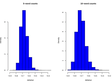
any level of significance. From Figure 1 it is also clearly evident that the bootstrap
distributions of ˆδ’s lie entirely to the left of zero, indicating a strong support for
underdispersion. These bootstrap distributions and corresponding estimates are
based on B = 5000 samples. We study the power of ˆδ in detecting the nature of
deltahat
Density
−0.9 −0.8 −0.7 −0.6 −0.5 −0.4 −0.3
0246
5−word counts
deltahat
Density
−0.9 −0.8 −0.7 −0.6 −0.5 −0.4 −0.3
0123456
10−word counts
Figure 1: Bootstrap distribution of ˆδ’s.
4.2
A Simulation study
In this section we generate data sets of size n from three discrete distributions:
(a) Binomial(m,mμ) (an underdispersed distribution), (b)P oisson(μ) (an
equidis-persed distribution) and (c) ZIP(p,1−μp) (an overdispersed distribution). Here
ZIP(p,1−μp) denotes a zero inflated Poisson (ZIP) distribution which is a special case of zero-altered Poisson distribution with δ=√pand f0 ∼P oi(1−μp) (see (1)). Notice that μ > 0 is the mean of each of the three distributions. We fix μ = 1
for all three distributions and choose m = 3 and p = 2/3 for non-equidispersed
models; these choices being motivated by the above real data. Notice that by
Bin(3,1/3) P oi(1) ZIP(2/3,3/√2)
n= 30 ˆ
δ -0.643 -0.156 0.764
s.e.(ˆδ) 0.185 0.347 0.225
0∈95% C. I. 0.336 0.865 0.487
n = 100 ˆ
δ -0.663 -0.079 0.805
s.e.(ˆδ) 0.084 0.288 0.053
0∈95% C. I. 0.040 0.914 0.007
n = 500 ˆ
δ -0.665 -0.037 0.814
s.e.(ˆδ) 0.033 0.208 0.020
0∈95% C. I. 0.000 0.928 0.000
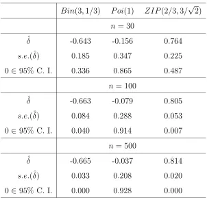
Table 3: Results based on simulation study
that the true value of δ is about 0.6647 and 0.8165 for the chosen binomial and
ZIP distributions, respectively (see the examples in Appendix A).
We present results for n = 30,100 and 500, which represents small, moderate
and large sample sizes, respectively, based on N = 1000 Monte Carlo (MC)
sim-ulations runs. To compute the standard errors and 95% confidence intervals we
used a bootstrap samples of size B = 500.
The results are summarized in numerically in Table 3 and graphically in Figure
2. In Table 3 we provide the average value (based on N = 1000 NC runs) of the
ˆ
δ obtained by using (6). We also provide the standard error estimate and the
proportion of times the 95% confidence intervals contained the null value δ = 0.
The standard error and 95% confidence interval (C.I.) estimates were obtained
by the bootstrap method. It is clearly evident as the sample size increases the
when n = 100, percentage of 95% C.I.’s that contained the null value 0 is about
4% under binomial sampling and is about 0.7% under ZIP sampling, whereas it is
about 91.4% under Poisson sampling.
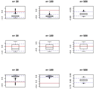
More insights can be obtained from Figure 2, where we present the boxplot of
the ˆδ’s along with the average values of the lower and upped bound of the 95%
C.I’s indicated by the dashed lines. The vertical axes of each plot has been set
the minimum and maximum of the lower and upper bounds of the 95% C.I.’s,
respectively. It is clear that the proposed method works remarkably well to detect
both underdispersion and overdispersion. Similar results were observed when
re-peated the simulation study with various other choices of the δ’s and underlying
distributions. As the procedure is semiparametric, the results were observed to be
fairly robust against a variety of assumed underlying distributions. A R code to
obtain ˆδ and associated C.I.’s can be obtained from the first author.
5
Conclusions
Zero-altered models have been shown to be useful for modeling outcomes of
man-ufacturing processes and other situations where count data with too few or too
many zeros are encountered. The proposed semi-parametric method of estimation
provides a flexible yet simple framework to model any discrete distribution with
finite second moment. Consistency and asymptotic normality of the proposed
es-timator makes it straightforward to apply the method in practice. Alternatively a
bootstrap method is found to be suitable for data with small sample size.
In the presence of covariates, proposed generalized zero-altered models can
be extended to include the effect of such predictor variables using suitable link
functions on δ. For instance, as δ ∈(−1,1), a Fisher’s z-transformation, given by
−1.0
0.0
n= 30
−0.8
0.0
n= 100
−0.80
−0.55
n= 500
−1.0
0.0
n= 30
−0.5
0.5
n= 100
−0.6
0.0
n= 500
−0.5
0.5
n= 30
−0.4
0.2
0.8
n= 100
0.70
0.80
0.90
n= 500
Figure 2: Performance of ˆδ: (a) first row is based on binomial sampling, (b) second
row is based on poisson sampling and (c) third row is based on zero inflated Poisson
sampling (for details see Section 4.2)
Acknowledgments The second author appreciates hospitality provided by the
Department of Statistics at NC State University, during his visit. The second
author’s work was supported by the Research Foundation of Chungnam National
References
Bailey, B.J.R. (1990). A model for function word counts, Applied Statistics, 39,
107-114.
Boos, D. and Stefanski, L. A. (2002). The calculus of M estimation,The American
Statistician,56, 29-38.
Cameron, A. C. and Trivedi, P. K. (1986). Econometric models based on count
data: comparisons and applications of some estimators and tests,Journal of
Econometrics, 1, 29-53.
Castillo and Perez-Casany (2005). Overdispersed and underdispersed Poisson
generalizations, Journal of Statistical Planning and Inference,134, 486-500.
Dahiya, R. C. and Gross, A. J. (1973). Estimating the zero class from a truncated
Poisson sample, Journal of American Statistical Association, 68, 731-733.
Efron, B. and Tibshirani, (1993). An Introduction to Bootstrap, Chapman and
Hall, New York.
Famoye, F. (1993). Restricted generalized Poisson regression model,
Communi-cations in Statistics - Theory and Methods, 22, 1335-1354.
Gupta, P. L. , Gupta, R.C., and Tripathi, R.C.(1996). Analysis of zero-adjusted
count data, Computational Statistics & Data Analysis, 23, 207-218.
Gurmu, S. (1997). Semiparametric estimation of hurdle regression models with
an application to Medicaid utilization, Journal of Applied Econometrics, 12,
225-242.
Hall, D.B. (2000). Zero-inflated Poisson and binomial regression with random
Heilbron, D.C. (1994). Zero-altered and other regression models for count data
with added zeroes, Biometrical Journal, 36, 531-547.
Heilbron, D. C., and Gibson, D. R. (1990). Shared needle use and health
be-liefs concerning AIDS: Regression modeling of zero-heavy count data, Poster
session, 6th International conference on AIDS, San Francisco, CA.
Hinde, J. and Demetrio, C. (1998). Overdispersion: models and estimation,
Computational Statistics and Data Analysis, 27, 151-170.
Huber, P. J. (1967). The behaviour of maximum likelihood estimates under
non-standard conditions, Proc. Fifth Berkeley Symp. Math. Statist. Prob., 1,
221-233.
Iverson, h. K. and Randles, R. H. (1989). The effects on convergence of
substi-tuting estimates into U-statistics and other families of statistics, Probability
Theory and related Fields, 81, 453-471.
Johnson, N. L., Kotz, S., Kemp, A. W. (1992). Univariate Discrete Distributions,
Wiley, New York.
Lambert, D. (1992). Zero-inflated Poisson regression with an application to
de-fects in manufacturing, Technometrics,34, 1-14.
Rao, C. R. (1965). On discrete distributions arising out of ascertainment,Sankhya
Ser. A, , 311-324.
Ridout, M., Demetrio, C. G. B., and Hinde, J. (1998). Models for count data
with many zeros, International Biometric Conference, Cape Town.
Tu, W. (2002). Zero-inflated data,Encyclopedia of Environmetrics,4, 2387-2391.
Umbach, D. (1981). On inference for a mixture of Poisson and a degenerate
Welsh, A, Cunningham, R., Donnelly, C. and Lindenmayer, D. (1996). Modeling
the abundance of rare species - statistical models for count with extra zeros,
Ecological Modeling,88, 297-308.
Winkelmann, R. and Zimmermann, K. F. (1995). Recent developments in count
data modeling: Theory and applications, Journal of Economic Surveys, 9,
1-24.
Yip, P.(1988). Inference about the mean of a Poisson distribution in the presence
Appendix A: Additional Results
Here we present conditions for the under, equi and over dispersion of X ∼ fδ
in terms of the first two moments of U ∼ f0. This extends the result given by Theorem 1.
Theorem 3. Suppose X ∼ fδ, where fδ is given by (1) and assume that the
underlying random variable U ∼f0 with σ02 <∞. The X is
under-dispersed i.e., μ > σ2 if δ <−δ0 equi-dispersed i.e., μ=σ2 if δ=δ0
and over-dispersed i.e., μ < σ2 if δ > δ0
where the cut-off value δ0 is a function of μ0, σ02 and π0 given by
δ0 = ⎧ ⎨ ⎩
μ0−σ2 0
μ2
0 if μ0 > σ
2 0
1−π0 π0 ·
σ2 0−μ0
μ2
0 if μ0 ≤σ
2 0
Proof: From Lemma 1, it follows that
σ2−μ= ω(δ)
μ2 0
(1−ω(δ))− μ0 −σ
2 0 μ2 0 .
As ω(δ)>0 ifδ <1, it follows that σ2 ≥μif and only if 1−ω(δ)≥(μ0−σ20)/μ20. But notice that,
1−ω(δ) = ⎧ ⎨ ⎩
δ2 if δ≥0
−δ2 π0
1−π0 if δ <0
.
Hence the result follows.
Next we show that under a mild condition any discrete distribution having
finite second moment can be represented by fδ(·) for some δ ∈ (−1,1) where the
Theorem4. LetX be random variable with pmfg(·)such thatμ=∞x=0xg(x)
and σ2 = ∞x=0(x−μ)2g(x) < ∞. Assume that g(0) +g(1) < 1. Then there is a unique δ ∈ (−1,1) and pmf f0(·) such that fδ(x) = g(x) for all x = 0,1,2. . .,
where fδ(·) is as given in (1) and μ0 =σ20.
Proof: Defineω =
1 + σ2μ−2μ −1
. Notice thatω >0 asE[X(X−1)] = μ2+σ2−μ > 0 by the assumption. Define,
f0(x) = ⎧ ⎨ ⎩
1− 1−ωg(0) if x= 0
g(x)
ω if x= 1,2. . .
(8)
Clearly,f0(·) defined by (8) is a pmf and it satisfiesμ0 =σ20whereμ0 =∞u=0uf0(u) and σ02 =∞u=0(u−μ0)2f0(u). Finally, δ can be obtained by solving the equation
δ2
+−δ2−1−f0f(0)0(0) = 1−ω. Notice that ω ≤1 if and only if σ2 ≥μ. Thus, it follows
that δ is given by
δ= ⎧ ⎪ ⎨ ⎪ ⎩ √
1−ω =
σ2−μ
σ2−μ+μ2 if ω≤1 ( i.e. σ2 ≥μ)
(ω−1)(1−g(0)) ω−(1−g(0)) =
μ−σ2
μ−σ2+ g(0) 1−g(0)μ2
if ω >1 ( i.e. σ2 < μ).
This completes the proof.
Some Examples:
(i) Suppose X ∼Bin(m, p), thenδ is given by
δ =
1 + m(1−p)
m
1−(1−p)m −1/2
(ii) Suppose X ∼P oi(λ), then δ= 0.
(iii) Suppose X ∼NegBin(m, p), thenδ = 1/√m+ 1.
(iv) SupposeX ∼ZIP(p, λ), thenδ =√p.