Semaphore queues: modelling multi-layered window flow control mechanisms

Revised Jan. '88

Semaphore queues:

Modelling multi-layered window

flow control mechanisms

by

s.

Fdida

1,

H.G. Perros- ', A. Wilk

3

lLaboratoire MASI, Universite P. et M. CURIE 4, Place Jussieu, 75252 PARIS cedex 05, FRANCE

2 Computer Science Department and Center for Communication and Signal Processing North Carolina State University,Raleigh, NC 27695-8206, USA

3 Polish Academy of Sciences, Dept. of Complex Control Systems ul. Baltycka 5,44-100 GLIWICE, POLAND

CCSP-TR-88/9 February 1988

ABSTRACT

We present an open queueing network for analysing multi-layered window flow control mechanisms consisting of different subnetworks. The number of customers in each subnetwork is controlledbya semaphore queue. The queueing network is analysed approximately using decomposition and

1 • INTRODUCTION

In a t.ypicallocal area network or wide area network, a data entity may have to traverse several layers of window flow. control mechanisms before it reaches its destination. In this paper, we present a model for analysing the delays introduced by such multi-layered flow mechanisms.

Pennotti andSchw~z[15] analysed a virtual route as a closed network of queues arranged in series, under the assumption of a loss system. That is, they assumed that packets that find a full window upon arrival at t?e system are discarded. Each queue represented a node on the virtual path. The effect of external amvals at each node was taken into account by reducing each service rate by the corresponding external arrival rate. Schwartz [23] extended this model to allow the case where the acknowledgements of transmitted packets are withheld until some proportion of the window has been received. Then, a single acknowledgement is sent back. Reiser [19] modelled a computer communication system consisting of many virtual routes with end-to-end window flow control, as a closed multichain queueing network. Each chain represented a different virtual route, under the assumption of a loss system. He proposed a computationally efficient approximation procedure based on mean value analysis for evaluating large closed multichain queueing networks.

Reiser [20] correctly observed that in real situations packets thatarrive to find a full window are not lost, but are queued in an input queue. Consequently, he analysed a virtual route with a sliding window as an open tandem queueing network. Associated with this network there was a pool of W tokens, where W is the window size. A customer can not traverse the network unless it has a token. A customer arriving at the network to find the token queue depleted, is queued in the input queue. Upon departure of a customer from the network, the token is returned back to the pool after a delay (acknowledgement delay). This queueing network was analysed approximately by reducing the network to a flow equivalent server, thus simplifying the analysis of the input queue. Varghese, Chou, and Nilsson [26] analysed the same open queueing model without an acknowledgement delay using the same approximation method. However, unlike the above paper, the service process of the flow equivalent server was characterized by a Coxian distribution. A good review of analytical methods for evaluating data communication systems can be found in Reiser [21]. More recently, Gihr and Kuehn [5] analyzed multi-layered protocol systems using hierarchical decomposition and aggregation techniques. The window flow mechanism was modelled as an open queueing system controlled by a pool of tokens, as described in Reiser [20].

Virtual routes with node-to-node window flow control have been modelled as open tandem configurations of finite capacity queues (see Caseau and Pujolle [3]). Each node on the virtual route is represented by a finite queue, whose capacity is equal to the node's window size. A server is said to be blocked if the next downstream queue is full. For further details and references on queueing networks with finite capacity see Altiok and Perros [1].

The problem of analysing window flow. control me~hanisms, ~an be formulated as a si!1~le or multiple class closed queueing network WIth a populatI?n constra~nt..Th.ese models w~re ongIn~lly developed for multiprogramming systems. Ifthe population cons!I"alnt IS lifted,.th~resultingqueueing

mechanisms permit for a more general type of population constraint. Finally. Goto, Takahashi, and Hasezawa [6] analysed an open tandem configuration with finite buffers and with an overall population constraint. This network permits the modelling of end-to-end and node-to-node window flow control mechanisms.

The problem of simultaneous resource possession arises in multiprogramming systems. In such systems, a job during its execution may require service from more than one server at the same time. This problem has been analysed using open or closed queueing networks (see Perros [16], Jacobson and Lazowska [7], and Freund and Bexfield [4]). A closely related topic, is the problem of serialization delays as arises in critical software sections and database locks. This model has been analysed by Agrawal and Buzen [2], Thomasian [24], and Jacobson and Lazowska [8].

In this paper, we present an open queueing network for analysing multi-layered window flow control mechanisms. These flow control mechanisms may be nested in any arbitrary way. This permits us to model node-to-node and end-to-end window flow controls. Also, each protocol layer at a switching node can be modelled by a separate queue, thus allowing us to represent delays introduced at each layer in a node. Each window flow control mechanism is modelled in a similar fashion as in Reiser [20] and in Gihr and Kuehn [5], through the means of a semaphore queue. The queueing models in this paper are analysed using standard hierarchical decomposition and aggregation.

This paper differs from other papers on window flow control in the following way. It deals with open queueing networks unlike papers [15], [20], and [23]. Papers [21], [26], and [5], deal with open queueing networks, but only one window flow control was considered. In papers [3], [1], and [6], each node is represented by a finite capacity queue, which implies a zero acknowledgement delay. This assumption was not made in this paper. Also, in these papers, the problem of multiple nested window flow control was not addressed. The problem of population constraint has mostly been analysed within the context of closed queueing networks. The open queueing models that have been proposed are either two-node models (see [16]), or require the assumption of a loss system (see [10]). Finally, the models reported for the analysis of simultaneous resource possession and serialization delays are either based on closed queueing networks, or they have been formulated specifically for multiprogramming systems.

In section 2, we introduce the concept of semaphore queue. An approximate solution to a queueing network involving one semaphore queue is given in section 2.1. In section 3, we give an approximation algorithm for analyzing a queueing network with multiple semaphore queues. This algorithm is validated in section4. A case study involving the modelling and analysis of the ISO

X25

flow control mechanism is given section 5. Finally, the conclusions are given in section 6.

2 • A QUEUEING NETWORK WITH A SINGLE SEMAPHORE

The management of a shared resource can be carried out efficiently using a semaphore. A semaphore station (S) consists of an input queue f'(S) and a token queue e(S). A customer arriving at the semaphore queue requests a token. The customer departs immediately, if there is a token available in queue e(S). Otherwise, the customer is blocked and it is forced to wait in the input queue f(S) until a token becomes available. Therefore, if there are tokens in etS), then there are no customers in the input queue. On the other hand, if there are customers in the input queue, then e(S) is empty.

f(S) ~

t .

J

Network 1

Network 2

Figure 1: A queueing network with a single semaphore

!n. figure ~, we introduce two symbols commonly used in Petri Nets in order to depict the fork and JOIn operation. Inparticular the join symbol

f(S) ~

e(S)

t· J

depicts the following operation. At the instance that queues f(S) and e(S) contain a customer each, the two customers instantaneously depart from their respective queues and merge into a single customer. The fork symbol

depicts the following operation. A customer arriving at this point, (i.e. departing from network 1) is split into two siblings. We use these two symbols for descriptive convenience.

2.1

THE APPROXIMATION ALGORITHM

Let us consider the queueing network described above and shown in figure 1. An exact analysis of this model is rather difficult. In view of this, we analyze it using decomposition and aggregation. In particular, we first analyze the system shown in figure 2 assuming that the arrival process at queue etS)is described by a state-dependent arrival rate y(k).

queue

reS)

t

j

Y (k)

queue e(S)

Figure 2: The semaphore queue

This queueing system depicts the semaphore operation described above. The arrival process at queue f(S) is assumed to be poisson distributed, and there are C tokens. We also assume that the inter-arrival times at queue e(S) are exponentially distributed with a rate y(k), where k is the number of outstanding tokens, i.e. C-k is the number of tokens in queue etS), The state of the system in equilibrium can be described by the tuple (i.j),where i is the number of customers in queue f(S) and j is the number of tokens in queue e(S). The rate diagram associated with this system is shownin figure 3.

iCC) Y(C)

~

A

YCc)

Figure 3: The rate diagram of the semaphore queue

We note that this system is identical toanMlMll queue with an arrival rate

A

and a state dependent service rate y(nq) ifn_g::;C, and y(C) ifn_q>C, where nqis the number of customers in this

MlMll

queue. The random variables i andj are _{related to nq as follows:} i = max (0, nq-C), j = max(0, C-n q).

The solution of this system is obtained by a direct application of classical results. Thus, we have

p(i,O)

=

pI

p(O,O) ,

I1(')

p(O,j)=

-~

p(O,O);

IJ

where p=

A /

y(C) and Fltj)=

. 1

n

y(C -k)

k=O

1

(1.1 )

,j > 0;

,j

=

0.

The probability

p(O,O)

is chosen so that the equilibrum state probabilities sum to 1:

1 C rr(jj

P(O,O)-l

= - +

I -

..

1 -

P

j= 1

AJ

From (2.1) and (2.2), we obtain the following marginal probabilities for each queue (index 1 is for queue f(S) and 2for queue e(S)) :

PI(D) = 1-

P

(1+ p(D,D))

1 -

P

PI (i)

=

pi p(O,O) ,

1

P2(O) = - p(O,O) ; 1 -

P

rr(j)

P2(j)

= - .

p(O,O) ,

IJ

i>

0;

(2.3)

(2.4)

Also, from (2.1) and(2.2) we can obtain PS(c), the probability that there are c customers in queue f(S) and in networks 1 and 2. We have

= { p(O,C-c), O~c ~C

PS(c) (2.5)

p(c-C,O) , c>C

Now, expressions (2.1) to (2.4) were obtained assuming that y(k) is known. This can be

appro~imately obtained by studying the closed queueing network (call it Q) obtained by linking queueing networks 1 and 2 as shown below.

Network 1

Network 2

The analysis of this queueing network can be carried out easily seeing that we have assumed that network 1 and 2 are of the BCMP type. Therefore, we can calculate the throughput of

Q

with k customers, where k= 1,2, ... ,C. This is then set equal to the arrival rate y(k) of tokens at the token queue e(S).

Let us consider for a moment the last queue in network 2, from which departing customers immediately join queue e(S). Let k' be the number of customers in this queue, and 1J.its service rate. Then Mailles [12] has shown that

Ap(O,j)

=

~(O,j-l) p(O,j-l)

where J.l.(i,j) = Jl[l- p(k' = 0Ii,j)]. The quantityy(k) can be seen as an approximation to Jl(i,j). We note that in the above formulation, the tokens are sent back via a separate network, network

2.

This formulation can be easily changed so that to allow the tokens to travel back over the network used by the customers, network 1. To do this, it suffices to declare two classes of jobs, namely class 1and class 2representing customers and tokens respectively. These two classes of jobs will then circulate within network 1 competing for the same resources. This network can be still modelled as

a

BCMPtype of queueing network as long the necessary BCMPassumptions are not violated.

Stability condition

The stability condition can be simply expressed as A<y(C), where y(C) is the maximum throughput of the network Q (see Lavenberg[11]) .

3 - A QUEUEING NETWORK vVITH lVIULTIPLE SEMAPHORES.

In general, \ve can regard a semaphore queue as the means of controlling the number of customers in a queueing network. Queueing networks controlled by semaphore queues can be combined by imbedding one network within another to make up larger more complex systems. In this section, we give a simple approximation algorithm for computing the solution of such multiple semaphore queueing networks. The algorithm can be used for any nested configuration involving

BCMP

queueing networks and semaphore queues. For presentation purposes, we consider the queueing network shown in figure 4. In this figure, SNi_,n-i=1,2,3,4 are fOUf arbitrary BCMP queueing networks, and Si_,n-I. i= 1,2, are two semaphore controlled queueing networks, as shown in

figure 5. The index n refers to a level of semaphore control. That is, the semaphore controlled queueing network shown in figure4,is associated with level n, and the one representedbySi,n-l,

i=1,2, is associated with level (n-l). Let _Cnbe the total number of tokens associated with the nth level semaphore controlled queueing network. Presumably, Si_,n-I. i=1,2, themselves may comprise of lower levels of semaphore queues. Likewise, level n may be imbedded in a higher level semaphore controlled queueing networks.

SN 3,n SN

4,0

U

f_{n (5)}

A-o-.

• •

_{• •}

_•

e_{n- 1(5)}

Figure 5: A level (n-I) semaphore subnetwork

Let us first consider the semaphore controlled queueing network S 1,n-1 as shown in figure 5. As in section 2, we can link networks Ql,n-1 and Q2,n-l to form a closed BCMP queueing network. This closed queueing network, call it Qn-1, can be analyzed using the MVA algorithm in order to obtain R'n-1 (k), the mean time to traverse Q1,n-1 as a function of the number of customersk in Qn-l' where k=1,2, ... , Cn-I. Similarly, we can obtain R"n-l(k), the mean time to traverse networks Ql,n-l and Q2,n-1 as a function of k, the number of customers in Qn-1. Using arguments as in section 2, we have that the rate "'{n-1(k) at which tokens return back to the token queue is approximately equal to k/R"n-1 (k), where k is the number of outstanding tokens. Hence, the mean response time R n-1(c) of a customer between points A and B, conditioned upon that he finds c customers (including himself) in queue fn-1(5) and in Qn-l upon arrival, is approximately given by

{

R'n-l (c), Rn-l(c)=

R'n-l(Cn-l)

+

_{(C-Cn-l)/Yn-l(Cn-1),}

c::;Cn-l

c~Cn-l,

(3.1)

The above expression can be easily derived. For, if c::;Cn-l' then all the customers are in Qn-l. Thus, our customer is delayed by R'n-l (c). If C>Cn-l, then only Cn-l customers are in Qn-l, and the remaining (C-Cn-l) are waiting in queue f_{n- 1(5). These customers depart from this queue} at the rate at which tokens return back to the token queue en-I (5), i.e. at the rate Yn-l (Cn-l)=Cn-l!R"n-1 (Cn-I)· A customer in queue fn-I (S), therefore, can be seen as receiving a mean service time equal to R"n-l(Cn-l)/Cn-l, before it enters Ql,n-1, where it is delayed on the average by R'n-l(Cn-I). Thus, we can obtain the above expression for Rn-l(c) when c~Cn-l·

consisting of Ql,n and Q2,n (call it Qn) areall BCMP queueing networks.

If the nth level semaphore controlled queueing network is itself imbedded in a higher level semaphore queue

«(

n+1)st level), then we can use the arguments given above in order to construct a flow equivalent composite queue. This composite queue will then be used in the (n+ l)st level semaphore network in order to substitute the original nth level semaphore network.

Now, let us assume that the nth level semaphore queue is the highest level. In this case, this queueing system can be analyzed using the arguments given in section 2. In particular, we

can

obtain p(i,j), where i is the number of customers in queue fn(S) and j is the number of tokens in queue en(S). Based on these probabilities we can obtain the mean response time, i.e. the

mean

time to go from U to V as shown in figure 4, as follows.

Let p(i) and q(j) be the marginal probability distribution that there are i and j customers in queue fn(S) and in queue en(S) respectively. Then, the mean number of customers in queue fn(S) is

Lfn(S)

=

L

i p(i) i=l

(3.2)

Now, let us consider queueing network Qn. Then, the mean number of customers in queueing network Q

1

_,n can be obtained as follows. Let

PI

(mlh) be the probability that there are

m

customers in Q1,n given that there are h customers in the closed queueing network Qn, and let

PI

(m) be the probability that there arem customers in Ql,n. For

mc-h,

we have

Pl

(mlh)=O.

For

0<m~h, we obtain

C_n

p.trn) = I p.tmlh) q(Cn-h)

h=m

Hence, the mean number of customers in QI n is_,

C_n

L_Q =

L

m Pl(m)

l ,n m=l

C_n

c

_n

=

L

m

(L

p.trnlh) q(Cn-h) )

m=l h=m

en

c

n

=

Iq(Cn-h)

L

mp.trnlh)

h=l m=l

m=l, ...,

en

The quantity

L

m

PI

_{(mlh), summed over m=l, ..,Cn, is the mean number of customers in}

QI

_,n given there are h customers in Qn. Now, the mean response time of Ql n as a function of the

C_n

L

m

PI

(mlh) =yn(h)

~(h)

- m=!

where Yn\h) is the rate at which tokens returnto the token queue, queue e (5). We have that Y (h)

IS appr?xlmately equal to hlR"n(h), where R"n(h) is the mean time to

tr~verse

Ql and Q7 nas

a function of h. Thus, .n z.n

C I

n Rn(h)

L

m p.tmlh)= h- ' -

I-m=! Rn(h)

and hence

(3.3)

We have expressed LQl,n in terms of the quantities R'nC·), R"n(·) so that to be consistent with the way we analyze each semaphore controlled queueing network. The mean response time between U andV is

1

R

=-

_A

[L_f (5) +L Q J

n l,n

where Lfn (S) and LQl,n are given by (3.2) and (3.3) respectively.

4 · VALIDATION

C3.4)

The approximation procedure described above was validated against exact numerical and simulation data. In particular, we analysed the model in figure 1 with a single semaphore queue, and the model in figure 4 with two and three levels of semaphore control. In general, the accuracy of the algorithm depends mainly on the utilization of the semaphore queue, expressed as the percent of time queue e(S) is busy, i.e.

I-p(O,C).

0.8

c:::

II

Approx

.2

_EI

Exact

"5 0.6 .c 'i:

en

-c ~ 0.4 C') c: ~ Q) ::s 0.2 Q) ::s 0 0.0

o

1 2 3 4 5 6

Figure 6: Queue-length distribution of the number of customers. Cl=3, A=.375, Jlll=Jl12=2

0.4 - . - . - - - ,

II

Approx.

El

Exact

iiiii

0.0 ... -c .2 'S 0.3 .c "i: u; "'C :E 0.2 en c: ~ ~ 0.1 Q) ::s o

o

1 2 3 4 5 6 7 8 9 1011

Figure 7: Queue-length distribution of the number of customers. Cl=3, A=.7S0,Jlll=~12=2

0.20

II

Approx

e

₀

_Exact

0 ";: _0.15 ::1 ..Q .;::

en

"'C

:c

0.10 C') e ~ ..9l Q) 0.05 ::1 Q) ::1 0 0.00

o

1 2 3 4 5 6 7 8 9 1 0 1 1 1 2 1 3 1 4

~~h semaphore utilization, the.approx~materesponse time is slightly overestimated. The relative

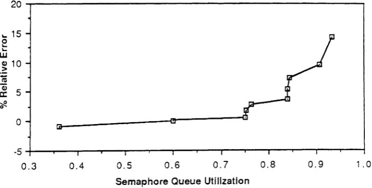
f or'·l~xpr.essedas 100(approXlmat~-slmulated)/approximate, is given in figure 10. We note that or un izanons of up to .85, therelativeerror is less than 5%.

I!J Approximate • Simulation 14 ms 12 Q) 10 E i= Q) ₈ en e 0 6 c, en Q) a: 4 c: co Q) :E 2 0

0.3 0.4 0.5 0.6 0.7 0.8

Semaphore Queue Utilization

0.9 1 .0

Figure 9: Mean response time vs semaphore queue utilization

1 .0 0.9 0.8 0.7 0.6 0.5 0.4

-5 -t--~_,---___T'-~-..,--.,.--,----...-...

-...---....---J

0.3 '- 15 o '-w ~ 10 .., co Qi a: 5 cf..

20 . . . .

-o

Semaphore Queue Utilization

Figure 10: % relative error vs semaphore queue utilization

for the results given in figure 9

Now, let us consider the model given in figure 4 with 2 levels, i.e. n=2. The semaphore

controlled queueing network S 1) is assumed to be the network analysed above. Networks SN 1,2 and SN2 2 are represented by a single server queue. As above, networks SN4 2 ' 52 1 and 5N 3 ") are omitted. Let C'2,

~

12,

~22,

and

A

be the window size, the service rate at the' queue representing SN1 '2 and at the queue representing SN'2.'2 ' and the total arrival rate at the inputlJueue. Figure 11 gives the approximate and simulated mean response time as a function of the utilization of the level '2 semaphore queue. Confidence intervals (95%) are also given for the simulation results. The

utilization ranging from .20 to .76. In particular, the parameters were varied as follows: C2=5,7, A=O.2, 0.6, 1,....Jl12= 0.2,0.5,0.8, Jl22= 0.2, O.?' 0.8; and Cl=3, Jll1~~12:=0.5. The rel~tive error observed is given in figure 12. We note again that for semaphore utilizations of up to

.8),

the relative error is below 5%.

6 ms

t:l Approximate

5

•

Simulation

C1) E t= Q) 4 en c: 0 c. CJ) 3 C1) c: c: ~ C1) ₂ ~ 1

0.2 0.4 0.6 0.8 1.0

Semaphore Queue Utilization

Figure 11: Mean response time vs semaphore queue utilization

15 . . . - - - ,

10 ~ 0

..

..

w Q) .~ 5 ~_Q) c: ~ 0 0 1.0 0.8 0.6 0.4

-5- + - - -...--....---...---.~-___r--___...--

...

- - - f

0.2

Semaphore Queue Utilization

Figure 12: % relative error vs semaphore queue utilization for the results given in figure 11

lower levels, i.e, levels land 2. The utilization of the semaphore queue of level 2 and 1ranged from .10 to .85. The results were obtained by varying the parameters as follows: C3=7, A=O.l, 0.6, .1, J.L13= 0.5, J.L23= 0.2,0.5,0.8; C2=5, J.L12=Jl22= 0.5; and Cl=3, J.Ll1=~ 12= 0.5. The

relative error observed for the mean response time for levels 1,2, and 3 is given in figure 14.

Again, we observe that the relative error is less than 5%for utilizations up to .85.We note that the relative error for the level 2 model is slightly higher than the one observed in figure 12. This is becauseofthe way the mean response time is calculated. That is, having analysed level

3,

we then work backwards using the standard disaggregation approach to compute lower level values.

15

ms _{m Approx. L3}

Q)

>Q) ₊ Simulation L3

-J

•

Approx. L2

~

(J _{0 Simulation L2}

ca

w 10 x Approx. L 1

~

ca _{6 Simulation L 1}

Q) E ~ Q) CJ) c: 0 ₅ Q. CJ) Q) a: c:

:=

('Q

g

I

OJ

HRR

:E a

0.1 0.2 0.3 0.4 0.5 0.6 0.7 0.8 0.9 1.0

Semaphore queue utilization

Figure 13: Mean response time vs semaphore queue utilization

25 - - - . ,

5

• %Rel Error L 1

EI %Rel Error L2

c %Rel Error L3

1.0

0.3 0.4 0.5 0.6 0.7 0.8 0.9

Semaphore Queue Utilization

0.2 0.1 1) ~ 20 -J ~ ~ 15 w loo. 10 o loo. loo. W Q) >

co

1) a:

Figure 14: % relative error vs semaphore queue utilization for the results given in figure 13

less than 5% for semaphore queue utilizations of up to .70 . For very high utilizations, the relative error exceeds 5%. However, it is not likely that such cases will be encountered in real life. Similar conclusions can be drawn for other nested configurations of semaphore queues.

5 • CASE STUDY: THE ISO X25 FLOW CONTROL MECHANISM

The past few years have seen important developments in the field of computer communication systems. The ISO reference model defined the protocol layers of a data network architecture. The philosophy of the ISO model lies on the service given by a layer and on the protocols designed for the achievement of each service. Each level delivers a service quality to the upper level and makes use of the service quality provided by the lower level. Thus, in a network: the purpose of each layer is to offer services to higher layers, shielding those layers from the details of how the offered services are actually implemented. Processes at each level run asynchronously. As a result of this, queues are formed at the layer interfaces. The complexity of these systems makes their analysis performance evaluation quite difficult. The queueing model analysed above appears to be easy to use and well suited for studying communication protocols. In this section, we employ this queueing network to model the flow control of an X25 ISO protocol.

The communication system under study consists of the first three layers of the ISO model, i.e. the physical layer, the data link layer, and the network layer (see figure 15). The physical layer (layer

HOSTA HOSTE

> ,

bits

physica1 channe 1 frames: "info"

<

:c::::: frames: "ack "

<:::: packets:" ackI I

_______

~IDQ.0~_siz~ _U!~ ~

_______

~ID~YJ~!_~~

_

packets : "fnfo " "'>

layer2

layer3

layer1

Figure 15: The X25 flow control mechanism

1) is concerned with transmitting bits over a communication medium.The task of the data link layer (layer 2) is to manage the data link control procedure responsible for the error correction over the physical channel. Layer 2 transforms the bit transmission facility into a line that appears to the network layer as being free of transmission errors.Three main frame types are used during a transmission phase: a) information frame (I), for transmitting information, b )receive ready (RR)

frame, for the positive acknowledgment of information frame, and c) reject (REJ) frame, for the retransmission of an erroneously transmitted information frame. The network layer (layer 3)

This communication system can be modelled using semaphore queues, as shown in figure 16. vVe assume a unidirectional communication from host A to host B. The external arrival of packets at host A is assumed Poisson distributed with parameter

A.

These packets represent the user/application packets. Let W2 and W3 be the window size at layers 2 and

3

respectively. An arriving packet joins queue f_3(S) if there are no tokens available in queue e3(S), When a token becomes available, the packet at the top of the queue is allowed to enter the layer 3 queue where it receives a service at the rate ~A3' Upon completion of this service, the packet joins queue f₂(S). When a token becomes available, the packet enters layer 2 queue where it receives a service at the rate J.lA" .This service includes the transmission time of a frame (which is a function of the frame length and the line capacity). Upon completion of this service, the frame joins an infinite server queue reflecting the propagation delay which is usually several times lower than the transmission time. (The probability of overtaking is assumed to be negligible.) Following this layer 1 service, the packet is assumed to be at host B. In particular, it joins host B layer 2 queue where it is served at the rate J.lB 1. Upon service completion, the frame may be rejected as being erroneous with probability

Pei-

In this case, a REJ frame is sent back and the frame is retransmitted. (We assume that an erroneous frame is simply retransmitted by the layer 1 server on a selective repeat basis.) With probability (l-Pei) the frame is found error-free and it is allowed to join the layer 3queue where it is served at the rate

u

B_{3. Finally, the frame upon completion of its service at the layer}

3

queue is delivered to host B. At the same time, a token (representing an RR frame being transmitted back) is placed in queue f₂ (S). The token is returned back, after transmission and propagation delay, to queue e3(S) through a path which is similar to the forward path followed by

the frame.

11I2 (1 2(8)

~I---'

packets RR

(

framesRR frames REJ

)

Pea

_ _ _ _ _ _ _ _~ (frame3RR

G(I~?1l1J2

~

framesREJ

packets I fram.e3 I) : 4 (

I

Pei

f (S)lJJ3 ) ~

ro--.,

~:Jm ~~

~:~

:

illD: 1

~l----~

.

.-~(8)

: : : : l-Pei

e₃(8)1 : A : tp : B :

" ' I I I I

1-Pea. I I I I

,...-.---.:

1:~

:

:~

I. __..I L. - - ..I

layer3 layer 2

Figure 16: The queueing model of X25 flow control mechanism

The service times of the customers in each of the que,:es in ~i&.u~e 16 are assumed to be

exponentially distributed. (This assumption is not necessary tor themhm~e server queue~).We~also assume that each layer is managed by a different processor. Layer 2 (link level) consls.ts or two

S namely a transmit and a receive queue. These two queues are served by the link layer

queue , . . f h . \ I d 1 th

;\1 PRl

r

&

;\1 FIFO

@

I I I I

'"

1

i

I I I I

I

",r

--+

II

..

:>

I

i\2 P R 2 & ~2 FIFO

@

I I I '"

"'2

i

..

I I I I

I

I-l!

--+

~

I. _ _ _ _~

Figure 17: Decomposition of the priority queueing model

can be done approximately following Schmitt [22] as shown in Gihr and Kuehn [5]. In particular, these two queues can be decomposed into the individual queues shown in figure 17 withJll

*

=

~l

and Jl2* = 1-12 (1 -a), where a is the probability that a customer entering queue 2 finds queue 1 busy.

a

is approximated by the following expression:

a= - ,

where

A

1 is given by the expression:

{

A/

(1- Pea)' for host A;

A /

(1- Pei) , for host B.

We now proceed to apply the approximation procedure described in section 3. In particular, we first analyze the subnetwork controlled by the semaphore queue [2 (S). This is shown in figure 18, where J.l*2

=

_J.lA2(I-a) and J.l*1 = J.l.B_1,and tp is the mean service time in the infinite server queues. The mean response time between points A and B in figure 9, R_2(c), c=1,2, ... ,W_3'can be obtained using expresion (3.1). Thus, this semaphore subnetwork can be substituted by a flow-equivalent infinite server queue with a state dependent mean service time equal to R_2(c).

Fol-tp

Figure 18: The link level semaphore subnetwork

substituted by-a similar flow-equivalent infinite server queue with a state dependent mean service nme equal to R2(c), c ~ 1,2, ... , W_3.The queueing network given in figure 16 can now be reduced to the ne~work shown In figure 19, which can be analyzed using the procedure outlined in section 3.

In

particular, we analy~ed.this queueing network in order to obtain a) R, the mean response time betweenPOIll~SU and V IIIfigure 19; b) T, the mean waiting time in the input queue [3(5); and c) X, th~mean time to traverse queues 1,2, and 3 (i.e. X=R-T). These quantities were computed as a function of

A,

W2, W3, the line capacity, and the bit-error rate.

W3

2

3

U

V

A

--0--+

JIll]

_~

•

f₃(S )

R_2(·)

IIIIJ

e3(S)

Figure 19: The level 3 semaphore network with aggregation

The following values were assumed for the input parameters: line capacityv=4.8~ 19.2,48 kb/s:

information packet size L=1072 bits; RR acknowledgement frame size 1=72 bits; RR and REJ frames 1'=~8bits; bit errorprobabilitv from which Pei and Pea are derived are set to 10-7,10- 5and 10-4;service times 1/JlA3=lms, 1/Jll33=1.5ms, 1/JlA₁= l/~El = (2

+

l'/v) ms, I/JlA₂₌₍₁

+

L/v )ms, 1/JlB₂₌₍₁

+

l/v )ms; line propagation time for a 4.8 kb/s line capacity tp = lIms, for a 19.2 or 48 kb/s line capacity tp

=

4ms.

The results obtained are presented in figures 20 to 24. Figures 20 to 22 show the int1uence of both layer 2 and layer 3 window sizes on R, T and X, and figures 23 and 24 give R as a function of the bit error rate and the line capacity respectively.

Figure 20 gives R as a function of the window sizes W3 and W2 for various values of the arrival rate

A

(expressed in packets/s).We note that as

A

increases, R increases as well. Also, for fixed value of W3, R decreases as W1 increases. Finally, for large values of

A,

increasing W3, while W 2 is kept constant, makes R increase slightly. This is due to the fact that more packets are competing for the same set of limited resources, and as a consequence X increases faster than T decreases. Thus, we have to limit the value of both windows in order to keep R small and to limit the number of resources used as buffers. For the given input parameters, it appears that a good choice of the two window sizes is: W3=3 and W2=2.

Figure 21 gives similar results as figure 20, but for X. We observe that for high values of

A,

X increases as the two window sizes increase.

Figure 22 gives R, T, and X as a function of the two window sizes W3, and.W~,where R

=

T

+

X. As the two window sizes increase, X increases and T decreases. ThISIS because, more customers are allowed in the semaphore controlled network, which makes the delay inside the network to increase, and the waiting timeinthe input queue to decrease.

when the bit error rate is 10-7 (respectively 10-4) no substantial improvement on R is obtained for values of the two window sizes on the right-hand side of (6,3) (respectively (3,3)). Thus, as the bit error rate increases, we have to limit both window sizes.

Finally, figure 24 gives R as a function of

A

for three different line capacities. This figure emphasizes the influence of the access line to the network, whose speed can be an order of magnitude lower than the network delay.

750

650

-a- A = 1

550

....

A=5

U) ₄₅₀

...

A =10

g

-0- _{A =12}

a: ₃₅₀ A =15

250

150

50

-~~-N~~N~~~N~~~~N~~~~-N~~~~~

~~N~~~~~~~~~~~~~~~~~~~~~~~~~

Window sizes (W 3W~

500

-e- A = 1

...

A=5

400

....

A =10 -0- _{A =12} A =15

300

en

S

>< ₂₀₀

100

~-N~NM~NM~~NM~~-NM~~~~NM~~~~

~~~~~~~~~~~~~~~~~~~~~~~~~~~~

Window sizes (W

3W~

Figure 21: X vs (vV3,W2) for different values of the arrival rate

A.

(packets/s); line capacity=19.2 kb/s, bit error rate =10.7

800

700

600

u;- ₅₀₀

S

I- ₄₀₀

r:i

x

300

200

100

0

_ _ ('! _ ("-.! M ~ ('~ ~ ~ ~ N M ~ ~ .- N M ~ ~ \0 . - N M ~ ~ \C ~

~NN~~~~~~~~~~~~~~~~~~~~~~~~~

Window sizes (W

3

W )2

1000

-6- 10 -7

800

...

10 •5

10 -4

600

en

g

a: 400

200

a

--N~N~-N~~-N~~~~N~~~~~NM~~~~

~~~MMM~~~~~~~~~~~~~~~~~~~~~~

Window sizes(WjW~

Figure 23: R vs (W3,WZ)

for different values of the bit error rate:

10-

7_{, 10-5,10-4 ;} arrival rate

A

=

12 packets/s, line capacity =19.2 kb/s

800

I!J 4.8 kb/s

•

19.2 kb/s

600

•

48 kb/s

en

g

400 a:

200

::=::

•

---0

0 5 10 15 20 25 30

Arrival rate A

Figure2-1: Rvsarrival rate

A

(packets/s)

6. CONCLUSIONS

In this paper, we presented a queueing network model, where the population within each subnetwork is controlled by a semaphore queue. The queueing model was analysed approximately using hierachical decomposition and aggregation. The analysis was restricted to the case of nested subnetworks. Clearly, the same approximation is aplicable to the case where subnetworks (or nests of subnetworks) are arranged in tandem. Each subnetwork was assumed to be of the BCMP type. The queueing network analysed in this paper, was employed to model the ISO X25 flow control mechanism.The influence of the window mechanisms on the mean response time was shown in a number of figures. Finally, the reader is referred to [9] where the end-to-end delay in a catenet environment is analysed.

REFERENCES

[1] T. Altiok and H.G. Perras, "Approximate analysis of arbitrary configurations of open

queueing

networks with blocking," Annals ofOpere Res.,voL9, pp. 481-509, 1987.

[2] S.C. Agrawal and J.P. Buzen, "The aggregate server method for analyzing serialization delays in computer systems," ACM TOCS, voL, pp.116-143, 1983.

[3] P. Caseau and G. Pujolle, "Throughput capacity of a sequence of queues with blocking due to finite waiting room," IEEE Trans. Soft. Eng., voL SE-5, pp. 631-642,1979.

[4] D.J. Freund and J.N. Bexfield, "A new aggregation approximation procedure for solving closed queueing networks with simultaneous resource possession," in Proc. ACM SIGlvlETRICS Conf., Minneapolis, Aug. 1983, pp. 214-224.

[5] O.Gihr and P.I. Kuehn, "Comparison of communication services with connected-oriented and connectionless data transmission", in Proc. Int. Seminar on Computer Networking and

Performance

Evaluation,Tokyo, Japan, Sept. 1985.

[6] K. Goto, Y. Takahashi, and J. Hasegawa, "An aproximate ananlysis of controlled tandem queues," inProc.lnt. Seminar on Modelling and Performance Evaluation Methodology,

Paris,

France, Jan 1983.

[7] P.A. Jacobson and E.D. Lazowska, "Analyzing queueing networks with simultaneous resource possession," Comm. ACM, vol. 25, pp.142-151, Feb. 1982.

[8] P.A. Jacobson and E.D. Lazowska "A reduction technique for evaluating queueing networks with serialization delays," PERFORMANCE

'83,

Agrawala and Tripathi (Eds.) , North Holland, 1983, pp. 45-59.

[9] U. Koerner, S. Fdida, H.G. Perras, G. Shapiro, "End to end delays in a catenet environment," in Proc. Third International conference on Data Communication Systems and

their Performance, Rio de Janeiro, Brazil, June 1987, pp 453-464.

[10] 5.5. Lam, "Queueing networks with population size constraint," IBM J. Res. Develp.,vol. , pp 370-378, 197.

[11] S.S. Lavenberg, "Stability and maximum departure rate of certain open queueing networks having capacity constraints," RAlRO lrforrnatiquettlomputer Science, vol. 12,

pp.353-370,

1978.

[12] D. Mailles, "Files d'attende descriptives pour la modelisation de la synchronization dans

les

system informatiques", These d'Etat, Univ. Paris 6, Sept. 1987.

[13~ D. Mailles, S. Fdida, "Queueing Systems with Flag Mechanisms": Proceedings of the International Workshop on Modelling Techniques and Performance Evaluation, Paris 87, North Holland, pp. 167-190.

[15]

[16]

[17]

[ 18]

[19]

[20]

[21]

[22]

[23]

[24]

[25]

[26]

:NLC. Pennotti and M. Schwartz, "Congestion control ill store and forward tandem links," IEEE

Trans. Comm., vol. COM-23, pp. 1434-1443,1975.

H.G. Perros, "A symmetrical exponential open queue network with blocking and feedback,"

IEEE Trans. Soft. Eng., vol. SE-7, pp. 395-402, 1981.

H.G. Perros, "A two-node queuing network with a maximum number of allowable jobs,"

PERFORMANCE '83, Agrawala and Tripathi (Editors), North-Holland, 1983, pp. 33-44.

D. Potier, "New user's introduction to QNAP2", INRIA tech. rep. 40, Feb. 1984.

M. Reiser, ".LL\ queueing network analysis of computer communication networks with window flow control." IEEE Trans. Comm., vol. COM-27, pp. 1199-1209,1979.

M. Reiser, 'IAdmission delays on virtual routes with window flow control," in P roc.

Performance of data Communication Systems and their applications, Pujolle (Ed.), North-Holland .. 1981, pp. 67-76.

M, Reiser, "Performance evaluation of data communication systems," Proc. [EEE .. Yo1.70,pp 171-196, 1982.

\V. Schmitt, "On a decomposition of Markovian priority queues and their application to the analysis of closed queueing networks," PERFORlv/ALYCE '84, Gelenbe (Ed.), North Holland, 1984, pp. 393-407.

M. Schwartz, "Performance analysis of the SNA virtual route pacing control," IEEE Trans. Comm., vol. COM-30, pp. 172-184, 1982.

A. Thomasian, "Queueing network models to estimate serialization delays in computer systems," PERFORMANCE '83, Agrawala and Tripathi (Eds.) , North Holland, pp.45-59, 1983.

A. Thomasian and P. Bay, " Analysis of queueing network models with population size constraints and delayed blocked customers," in Proc. ACM SIGMETRICS Conj., Cambridge, 1984, pp. 202-216.