Sensitivity to color errors introduced by processing in different color spaces

Sensitivity to Color Errors

Introduced by Processing

in Different Color Spaces

Robert E.

Van

Dyck

Sarah A. Raj ala

Center for Communications and Signal Processing

Department Electrical and Computer Engineering

North Carolina State University

TR-91j9

Sensitivity to Color Errors Introduced by

Processing in Different Color Spaces

Robert E. Van Dyck

Sarah

A.

Rajala

Center for Communications and Signal Processing

North Carolina State University

Raleigh, NC 27695-7914

April 10, 1991

Abstract

To achieve the desired compression ratio, most coding methods employ some type of quantization. When processing color images, this quantization leads to color errors. The subjective visual quality of compressed color images can be improved by transform-ing to and then processtransform-ing in a different color space. An iterative algorithm is derived that allows one to design one dimensional minimum mean squared error quantizers using a discrete histogram as input. The resulting quantizer is a close approximation to the optimal one. This algorithm is used to design the quantizers for each component of a color image or subimage. The minimum mean squared error criterion is, therefore, implemented in the color space component that is being quantized.

A test image stored as C.I.E. XYZ tristimulus values is transformed to an RGB space, an YIQ space, and L*a*b* space. These four images are both directly quan-tized and subband coded, where the quantizer for each component of each image or subimage is designed using the algorithm mentioned above. The results for a number of compression ratios and bit allocations are compared to determine which color spaces are better for compressing images.

1

Introduction

1-1

Color Spaces

With the exception of a few colors of high purity, all colors can be matched by a combination of three different color primaries [1]. By matched, it is meant that the additive combination of particular amounts of a red, a green, and a blue light appears the same to the viewer as a given color. The reason for this phenomenon is that the human eye has three different color sensitive receptors. The receptor responses are functions of the wavelength of the incident light and can be denoted by f3>.., I>", and

p)... The functions have maxima in the blue, green, and red regions of the spectrum,

respectively.

By matching a unit power amount of all colors of the spectrum with a particular set of a red, a green, and a blue color, three tristimulus curves can be created. The units of the tristimulus values are such that a particular white color can be matched by equal amounts of these three colors. The tristimulus curves are used to match colors as follows

This equation states that a unit amount of some color, C, containing many spectral colors can be matched by R; units of color R, G e units of color G, and Be units of color B. If the tristimulus values, Re, Ge,and Be are allowed to have negative values, then all colors can be matched.

A new color space was desired that would satisfy a number of criteria. The three primaries should be chosen such that all real colors could be matched by positive quantities of these three primaries. This implies that the primaries are outside the gamut of realizable colors. Also, the luminance of the color should be described by only one primary. This color space should also be a linear transformation of a color space containing red, green, and blue primaries. The resulting color space is the 1931 C.I.E. XYZ space, in which the Y component contains the luminance of the color. Tables of color matching functions have been defined so that the XYZ coordinates of any spectrum can be computed.

Starting from XYZ space, transformations to other color spaces have been defined. These color spaces include an RGB, a YIQ, and e.I.E. L*a*b* space. The first two are linear transformations of XYZ space and are versions of those used in broadcast color television. YIQ space, in particular, provides good energy compaction since the luminance component, Y, carries much of the information. The last color space results from a nonlinear transformation of XYZ space. It is considered to be a uniform color space since equal color differences correspond to almost equal visual color differences.

1-2

Color Space Processing

The typical color monitor or television set displays color images through the use of three electron guns. These guns are used to excite red, green, and blue phosphors, respectively. Although the display is in some RGB space, the processing, including coding and transmission, may be more efficiently done by first transforming this color

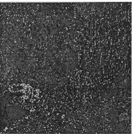
Figure 1: Luminance Component of Image

space to another one and then doing any required processing. This idea has been implemented in conventional color television where the three analog color signals are linearly transformed to a luminance and two chrominance signals, YIQ, to achieve bandwidth compression.

An underlying problem in all color image compression methods is the determination of the sensitivity of the human visual system to color errors. This is especially true in systems that are to provide almost visually lossless images such as HDTV systems. Studies done by MacAdam

[2]

and others show that the human visual system is not equally responsive to the same size color error in different parts of an RGB color space. One approach to this problem involves the transformation of the color space to a color space that has more perceptually uniform errors.

In this paper we investigate the effects of color image compression in different color spaces. The input is a test image that is recorded as a C.I.E. XYZ space tristimulus image. Figure 1shows a gray-scale version of our test image, created from the lumi-nance component. Much of the work focuses on subband coding since it provides a sufficiently general framework for study, while it is also a viable choice for high bit-rate applications.

The sizes of the color errors depend on the number of levels in the quantizer as well as the type of coder used. Gentile, et.

at

[3], have performed experimental calculations of color errors for uniform quantizers with fixed step sizes for various color spaces. We

01 tne sensitivity ot tne numan visual system to color errors. This is especially true in systems that are to provide almost visually lossless images such as HDTV systems. Studies done by MacAdam [2] and others show that the human visual system is not equally responsive to the same size color error in different parts of an RGB color space. One approach to this problem involves the transformation of the color space to a color space that has more perceptually uniform errors.

lumi-quantizers designed for each component of each subband in the latter case.

2

Distortion Measures

Much of the original work in evaluating the sensitivity of the human visual system to luminance errors use a model of the visual system to compute various distortion measures [4] [5] between an original and a processed image. Many of the models of the human visual system assume that there is an initial nonlinearity, followed by a linear system that is frequency and orientation dependent [6]. Subjects were asked to judge the quality of the images and the subjective rating was then compared to the distortion measure to determine the usefulness of the latter. This line of work has since been extended to color images [7]. A result of this work is that one can obtain a better distortion measure if the original image and the processed images are first transformed to a perceptually uniform color space and the distortion measure is calculated in this space.

To extend this approach to processing in different color spaces, the input image is transformed into another color space, coded and decoded in that space and then trans-formed back to the original space. The input and output images are then transtrans-formed to a uniform color space and the distortion measure is calculated. We implemented this method because it is mathematically tractable and because it provides an initial numerical assessment of the coding algorithms. L*a·b* space was used as the uniform color space. (~L*)2

=

(Lt - L~)2, (~a*)2

=

(ai - a~)2, and (~b*)2

=

(bi - b~)2,

where the subscripts i and 0 refer to the input and output images, respectively. The

distortion measure is ~E, given by

This distortion measure was computed on a pixel by pixel basis to provide error images. These error images are more useful than an average value of ~E for an image since they show where the distortion is above a visible threshold.

3

Color Transformations

3-1

Display of XYZ Image

3-1.1 Image Characteristics

An image of a toy store of size 1365 X 1365 pixels was recorded in XYZ tristimulus values. Each pixel is stored with 16 bits of accuracy. Two 256 X 256 windows of this image were chosen to be our input images. The first one consists primarily of a girl's face and was picked so that the coding algorithms could be tested on fleshtones. The second image contains a number of saturated colors and is used to test how accurately the coding algorithms can code these type of images.

3-1.2 Gamma Correction

Our color display monitor uses 24 bits per pixel to represent color images. Eight bits per pixel are used to store the red, eight for the green, and eight for the blue. Consequently, each component can take on values from 0 to 255. Although the image in XYZ is the basis for our simulations, we need to be able to transform it into the red, green, and blue coordinates of our display. We shall call this color space Display RGB to distinguish it from the RGB space that we process in. Using a colorimeter, we are able to measure the XYZ values transmitted from our display. Since we want these measured values to agree with the internal values, the transformation from XYZ to Display RGB must also take into account the nonlinear transfer functions of the three electron guns. This is known as gamma correction.

To do this, the color display is characterized by six parameters. These include the values of gamma for each of the three colors, and the minimum visible pixel values, no, for each color. These parameters were experimentally determined and are as follows

IT

=

2.310

19

=

2.237

Ib= 2.200

nOr

=

23.56

nOg

=

30.47

nOb

=

29.61

The gamma correction is done by the nonlinear transformations

RD

=

(255 - nor)r1/')'r

+

nOr GD = (255 - nog)gl/')'g

+

nOg

BD

=

(255 - nob)b1/')'b

+

nOb

where the subscript, D, refers to the displayed values. The rgb values are obtained from a linear transformation of XYZ space. This transformation is monitor dependen t and in our case is given by:

All of the rgb values lie between zero and one.

3-2

Transformation to

RGB

The mapping from the XYZ tristimulus values to the RGB values is a linear transfor-mation that is based on the NTSC phosphors. It uses standard illuminant C as the white point and is given by [8]:

[

~

B

] =

[-~:~~~~ -~:~~~~ =~:~~~~]

0.0583 -0.1184 0.8980

[; ]

Z

The minimum tristirnulus values are zero and the maximum tristimulus values are

[

X]

Y_Z

=

[

_48.4345.15 ]48.90

max

3-3

Transformation to

YIQ

The transformation from XYZ to YIQ space takes place in two steps. The first step is the transformation from XYZ to RGB shown above. The second step is from RGB to YIQ. This is a linear formulation of the NTSC transformation.

[

~

_Q

] =

[~:~~: -~:~~~ -~:~;~] [~

_{0.212 -0.523 0.311 B}

]

3-4

Transformation to

L *a*b*

L*a*b* space is an almost perceptually uniform color space created by a nonlinear transformation of XYZ space. The transformation needs the XYZ coordinates of the desired white point. In our simulations, we used 90 percent of the white point of our display. When the maximum red, green, and blue values of 255 were input, the output color is the display's white point. This was transformed to XYZ space, and reduced by 10 percent to allow color errors that are both above and below the white point.

The transformation from XYZ to the CIELAB color space L*a*b* is given by the equations [9]

L*

=

116(Y/lr

o)1/3 - 16

a*

=

500[(X/ X_{o)1/3 - (Y/Yo)1/3]}

b" = _{200[(Y/Yo)1/3 -} (Z/Zo)1/3]

where X o, Yo, and Zo are the tristimulus values of white. These formulae are only correct for values of X / X_o, Y/Y_o,and Z / Zogreater than 0.008856. For lower values of these ratios, L*

=

903.29(Y/Yo), and a" and b" are also changed.

4

Quantization

We needed a method to design quantizers for each color component of an image. Max showed [10] that to find the optimal quantizer for the one dimensional signal given by the probability density function, Py(y),using a minimum mean squared error distortion criterion, one had to simultaneously solve the nonlinear equations

and

Tk

+

Tk-l

tk

=

-2

where the tks are the decision levels and the

Tk

s are the reconstruction levels.

Pantera~d Dite [1i] derived a nearly optimal quantizer by assuming that the num-ber ofqua~tlzerlevels IS large enough that the probability density function is constant

for the region between two consecutive decision levels. This assumption leads to the following equations

and

tk+l

+

tk

Tk

=

-2

where A

=

t£+l - t1 , Zk

=

kA/ L, L is the number of levels, and k

=

1 ...L.

The first of these two approximate equations is formed by taking the continuous approximation to the series

A 2 2 2

tk

=

R"" [ 1/3( )

+

1/3( )

+···+

1/3( )]

+

tl

P T1 P T2 P Tk-l

where K is the normalization constant

This equation can be used instead of the integral to directly calculate the decision levels.

We modified the method of Panter and Dite by making it iterative. A histogram was used as an approximation of the probability density function. The bin size was selected so that there were roughly 100 bins containing nonzero samples. The minimum and maximum values for the quantizer range were selected. In most cases these were the points where the tails of the distribution went to zero. In some cases, however, a few outlying points were discarded. As presently implemented, this is necessary for convergence. The algorithm can be further refined so that these points are included. In either case, the number of excluded points was so small that it had a negligible effect on the results.

The zeroth pass through the algorithm creates a uniform quantizer with the lowest decision level at the lowest bound and the highest decision level at the highest bound. The probability density function is averaged between each decision level and these values are used in the series for Tl through TL. The averaging acts as a smoothing function and helps insure convergence. Using the midpoint value, as Panter and Dite originally did, leads to less stability in the algorithm. After the decision levels are calculated, the reconstruction levels are found and the iteration is complete. Instead of using the uniformly distributed decision levels, these new ones are used as the inputs to the next iteration. The mean squared error is calculated at the end of each iteration, and is used to determine which set of levels is best.

The algorithm is run until convergence is achieved. Because of the discrete nature of the histogram, the levels will usually oscillate between two sets. This generally occurs after less than twenty iterations. The iteration with the lowest mean squared

error is chosen. This is not necessarily one of the last ones. Often, after only two or three iterations a minimum is achieved. The final values are usually slightly higher. While there is no guarantee that this is the global minimum, for smooth distributions the results are considerably lower than the uniform case.

5

Subband Configuration

In monochrome subband coding, an image is spatially filtered into a number of or-thogonal frequency bands. Each subband is then decimated so that the total number of pixels remains constant [12]. The subbands are separately encoded in a way that takes into account the properties of the human visual system to the frequencies in the subband. It is possible that some subimages contribute so little to the reconstructed image that their omission does not perceptually change the image. In this case, these subimages do not need to be transmitted.

The simulation that we implemented first filters the image into four subbands using the 32 tap filter known as 32D in [13]. One subband is a lowpass filtered version of the original, and the other three are bandpass filtered versions. The lowpass subimage is then filtered into four more using a 16 tap filter to yield a total of seven subimages. All filtering is done in the frequency domain. The subband coder was extended to color images by creating three such systems in parallel. Each system processes one of the three color components. This system is flexible enough to allow processing in alternative color spaces since the filter structure remains constant. The only change between color spaces is in the set of quantizers used.

6

Experimental Results

6-1

Quantization Results

The first test consisted of quantizing the image in the four color spaces using 4 bits/pixel/component. This is only a compression ratio of 2:1, but it still shows differ-ences among the color spaces. The ~E value is the lowest for L*a*b* space, which is not surprising since the quantizer design was run in this color space. The question is whether the visual appearance matches these average numbers.

The Lra'b" image shows contouring on the girl's face. Although the color errors

are quite small, this is somewhat objectionable. The XYZ space image has the highest

~E error by far. Most of the image is not too bad, except for one region on the girl's forehead where there are clearly visible color errors. The flesh appears to be green and red. The color error in this region is high enough to raise the average. Overall, the image is not good. The RGB image also shows similar color errors on the forehead. This space still appears to be better than XYZ space. The YIQ space had some of the same errors as L*a*b* space. For this reason, further tests where run on the latter space.

The first set of tests did not contradict the ranking obtained by the ~E distortion measure. This is somewhat unfair since we are using one of the test color spaces to

Color Space bits/pix ~ E (ave)

L*a*b* 5,4,4 1.801

4,4,4 2.340 5,3,3 3.517 4,3,3 3.880 XYZ 5,5,5 8.260 4,4,4 12.211

RGB 5,5,5 5.178 4,4,4 9.653 YIQ 5,4,4 7.583 4,4,4 7.762

Table 1: Distortion Measure Results

compute the distortion measure in. Even though it is almost a uniform space, some different, uniform space should be used instead. A color space whose transformation is too complicated for real-time compression, but whose results are perceptually uniform would be best. A number of such spaces exist and one may eventually be used.

The second set of tests consider only L*a*b* space. Three additional simulations are run. Table 1 shows how the bits were allocated to each color component. While the 4,4,4 case has a lower average distortion, the 5,3,3 case appears to be much better. By allocating 5 bits/pixel to the luminance component, the contouring on the girl's face is practically eliminated. The chrominance errors are barely visible, even in the highly saturated yellow area. A second test image that contains many saturated colors will most likely yield different results. Yet for fleshtones, this configuration is clearly superior. The 4,4,4 case and the 4,3,3 case do not look much different, again showing that the luminance tends to dominate.

Figures 2 and 3 contain DaE error images for these two cases. The value of DaE

at each pixel has been multiplied by twenty to make the errors more visible. An examination of these images shows that the spatial variation of the errors are different. In the 4,4,4 case, the errors are higher on her face where the contours appear. In the other case, the values ofDaE are lower there, but higher in the regions of saturated color. The error images match one's subjective judgement of the images in the sense that higher values correspond to a more visually noticeable error. However, this distortion measure is not ideal since the luminance error appears to be more visually important, while the distortion measure gives equal weight to each color component.

6-2

Subband Results

6-2.1

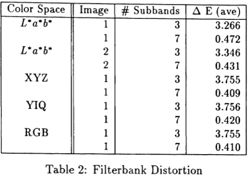
Filterbank Distortion

Table 2 shows the distortion caused by the subband filters for the case where only the three lowest bands and all seven bands are used in the reconstruction. In the seven band case, the average !i.E is well below the visual threshold of approximately three for all color spaces. In the three band case the average value is just visible. However, it

Color Space Image

_#

Subbands ~ E (ave)

L*a*b* 1 3 3.266

1 7 0.472

L*a*b* 2 3 3.346

2 7 0.431

XYZ 1 3 3.755

1 7 0.409

YIQ 1 3 3.756

1 7 0.420

RGB 1 3 3.755

1 7 0.410

Table 2: Filterbank Distortion

must be remembered that the average ~E figures do not account for spatial artifacts so that there will be regions in the image that have more color errors.

6-2.2 Subband Simulation

Because of the number of quantizers that must be designed to implement a 7 subband coding system, simulations were run for two L*a*b* cases and one YIQ case. The first simulation allotted a different number of bits to each subband, depending on the histograms of the subband's components. Between 5 and 2bits/pixel/component were allocated such that the overall compression ratio was approximately 2.5:1 (2.53:1). This yielded an averageD,.E error of 1.648, and an image that still showed some contours on

the girl's face. The second case was the same as the first except that 6 bits/pixel were given to each component of the lowest subband, instead of the 5 bits/pixel given in the first case. For a 2.56 x 256 image, the lowest subband is 64 x 64 so the compression ratio is only reduced to 2.48:1. The average DaE error is now 1.368, and the output image looks almost identical to the input.

The YIQ simulation used the same bit allocation as the second L*a*b* case. It had a f:J,.E error of 6.327. The contouring was not very visible, but a close examination of the image showed some color errors in the green. This may be partly do to the fact that our input image contains some scanning errors that appear as faint green vertical lines.

7

Conclusions

Initial simulation results show that the subjective image quality can be improved by transforming the input image to a uniform color space and implementing a subband coding system in this color space. The visual differences between this color space and other, linear transformations, of the input color space is noticeable but not too different for high quality images. However, as the bit rate is reduced, the uniform color space processing is more robust.

References

[1] R.W.G. Hunt, The Reproduction of Colour, John Wiley and Sons, New York, 1975.

[2] D.L. MacAdam , "Uniform Color Scales," Journal of the Optical Society of

Amer-ica,vol. 64, pp. 1691-1702, Dec. 1974.

[3] R.S. Gentile, J.P. Allebach, and E. Walowit, "Quantization of Color Images Based on Uniform Color Spaces", Journal of Imaging Technology, vol. 16, pp. 11-21, Feb. 1990.

[4] J.L. Mannos and D.J. Sakrison, "The Effects of a Visual Fidelity Criterion on the Encoding of Images," IEEE. Trans. on Information Theory, vol. IT-20, pp. 525-536, July 1974.

[5] Z.L. Budrikis, "Visual Fidelity Criterion and Modeling," Proceedings of the IEEE., vol 60, pp.771-779, July 1972.

[6] H. Mostafavi and D.J. Sakrison, "Structure and Properties of a Single Channel in the Human Visual System," Vision Research, vol. 16, pp. 957-968, 1976.

[7] O.D. Faugeras, "Digital Color Image Processing Within the Framework of a Hu-man Visual Model," IEEE. Trans on A SSP. , vol. ASSP-27, pp. 380-393, Aug. 1979.

[8] W.N. Sproson, Colour Science in Television and Display Systems, Adam Hilger Ltd, Bristol, 1983.

[9] G. Wyszecki and W.S. Stiles, Color Science: Concepts and Methods, Quantitative

Data and Formulae, John Wiley

&

Sons, New York, pp. 164-169. 1982.

[10] J. Max, "Quantizing for Minimum Distortion", IRE Trans. Information Theory, vol. IT-6, pp. 7-12, Mar. 1960.

[11] P.F. Panter and W. Dite, "Quantizing Distortion in Pulse-Count Modulation with Nonuniform Spacing of Levels," Proc. IRE, vol. 39, pp. 44-48, Jan. 1951.

[12] J.W. Woods and S.D. O'Neil, "Subband Coding of Images," IEEE Trans. on

ASSP, vol. ASSP-34, pp. 1278-1288, Oct. 1986.

[13] J.D. Johnston, "A Filter Family Designed for use in Quadrature Mirror Filter Banks", Proc. ICASSP, pp. 291-294, Apr. 1980.