SEMIANALYTICAL SOLUTION METHOD OF
DIFFERENTIAL-INTEGRAL EQUATION OF FLAT CRACK PROBLEM
Anatolii Batura1, Igor Orynyak2, and Andrii Oryniak3
1
PhD, Senior Scientist, G.S.Pisarenko Institute for Problems of Strength of National Academy of Science of Ukraine, Kiev, Ukraine ([email protected])
2
Professor, Head of Department, G.S.Pisarenko Institute for Problems of Strength of National Academy of Science of Ukraine, Kiev, Ukraine ([email protected])
3
PhD student, National Technical University of Ukraine “Kyiv Polytechnic Institute“, Kiev, Ukraine
ABSTRACT
The exact analytical approach for stress intensity factor calculation for an arbitrary shape mode I crack loaded by the polynomial stresses is proposed. The approach is based on the calculation of the crack faces displacement at given loading. At that the key problem is the solution of well-known inverse task: obtaining the stresses field at the crack faces on the base of a given displacements field. Multiply solution of such task for a whole set of certain displacements base functions (e.g., for the polynomial terms) allows to get analytical expression which connects stresses and displacements fields.
The original semi-analytical technique for integration with subsequent differentiation of well-known singular integral equation of the flat crack problem is developed. The excellent accuracy of the method is confirmed for an elliptic crack as well as for a rectangular one in the infinite 3D body. New results are given for an inner semi-elliptic crack in the infinite body which surfaces are loaded by polynomial stresses up to the 6th order.
INTRODUCTION
The key problem of the assessment of Nuclear Power Plant safety and residual lifetime is the estimation of allowable shift of the critical brittle temperature for the Reactor Pressure Vessel (RPV), in other words – the assessment of the brittle strength of reactor (thick-walled cylinder vessel) at different operation conditions, especially – at accidents. Obviously, that such calculations are impossible without Stress Intensity Factor calculation (SIF) for the postulated crack in the wall of RPV.
There is a lot of SIF calculation methods at present for the cracks of “canonical” shapes, e.g. semielliptical surface cracks, internal elliptical cracks. A large amount of interpolational expression of high accuracy was got for those cracks and such expression are widely used in the strength-assessment standards for nuclear, petrochemical, transport industry, etc. Also, such methods as Weight Function Method (e.g., see Orynyak et al. (1994)) allows to extend existing results for “canonical” cracks for the case of arbitrary loading.
However, according to the last approaches in the nuclear industry it is necessary to calculate SIF for the cracks with lack of theoretical base solutions, such as “eye-shaped” cracks in the rounding of the nozzle, internal (under-cladding) semielliptical cracks, etc (e.g., see VERLIFE (2008)). The most usual solution, included in the normative documents, is the interpolative tables, obtained by the Finite Elements Method (FEM). But question of their verification is still open, because there are no enough test data for the comparison.
The relation of SIF and crack faces displacements field at crack contour zone is the well-known result of the theory of elasticity, e.g. Panasyuk (1988), eqn. 1.24. This relationship for the close proximity of crack contour can be written in the following form:
G K
U I
2 1 , (1)
where U - is the crack face opening in certain point (x, y), - the length of the normal from (x, y) to the point of crack contour, - Poisson's ratio, G - shear modulus, KI - SIF in the correspondent point of
crack contour.
From the form of (1) the quite simple conclusion can be made: an expression for the KI is the
limit transition of expression like U/const at 0. So, the main goal of the presented work is to
find the expression for crack faces displacements field U
x,y on the base of arbitrary stress field in the form applicable to such transition.THE IDEA OF THE METHOD
The method is based on the well-known theoretical solution of the task, which is an inversion of current: finding of the stresses field for the crack faces on the base of certain displacements (crack face opening) field. The singular differential-integral equation for this task is known (see Panasyuk (1968)):
S x y
d d U y
x E
y x p
2 2
2 2 2 2 2
, )
1 ( 4 ,
, (2)
where (x, y) and
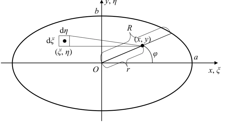
, are Cartesian coordinates in the crack plane related to the some point of the coordinates origin, say point O (the example, elliptical crack, is shown on Fig. 1); p(x, y) is the load acting on the crack faces; S is the crack area;E
is the module of elasticity.x
,
ξ
y
,
η
R
r
d
ξ
d
η
O
(
x
,
y
)
(
ξ
,
η
)
a
b
φ
Figure 1. Coordinate system and nomenclature for the elliptical crack.
In spite of this relatively simple formulation of the flat crack problem (2) there are no universal
they either employ a very complicated techniques, for example, Fourier transform (Stadnik and Gorbachevskiy (1981)) or the main (singular) part is extracted from the above hypersingular integral equation which is solved analytically while the remained part of it is solved numerically (Qin and Noda
(2003), Tang and Qin (1993)). Furthermore, obtaining of the general inverse (which is actual for our goal)
solution of (2) in the close form seems to be impossible.
Thus, the idea of the solution method is that: expression (2) is replaced by its analytical interpolative function in the form that allows easyobtaining of the inversion. Then obvious step should be made. This method requires determination of (2) values through the S to find the interpolation.
A polynomial interpolation of (2) is proposed to use. It can be relatively easy obtained and transformed into the inversion. Also the accuracy of calculation can be increased by obtaining the interpolation for the integral part of (2) and further analytical application of Laplacian (double differentiation in (2)).
The dimensionless shape function is commonly used at crack problem calculations for taking
into account asymptotic character of crack face opening at contour proximity, which is proportional to
according to the common solution of fracture mechanics (see expression (1)). Note, that such
character can be hardly replicated by the polynom.
The choice of the form is quite complex and ambiguous task which should be solved
individually for different types of the crack shape. The following function was decided to use it this
work because of its generality, good correspondence to the real opening shape for the well-known types
of crack (e.g. elliptical, rectangular), also limit transition
lim0 /
U can be trivially obtained for it:
) (
) (
1 2
2
R
r
, (3)
here - is the angular coordinate of a point, r
– radius to the point from the crack center (coordinates origin), R
– radius function, which describes crack contour (see Fig. 1). Note, that geometrical center of the elliptical and rectangular cracks can be trivially chosen as their coordinates origin, unlike certain other cracks, such as semielliptical, where choosing the geometrical center is ambiguous task.The expression (3) is not the only possible type of . E.g., in several literature sources another
is used for the rectangular crack (see Qin and Noda (2003)):
2 2 2
2
1 1 1
a b
. (4)
In general, this expression is rather strange, because polynom degree under root sign depends on the proximity to the corner of crack contour and can change from 2 near the center of rectangular side to 4
near the corner or even to a higher value if several corners are close to each other. So, expression in
form (3) is more reasonable than (4).
According to the above, the interpolative form of displacements U and stresses p are the
following:
,
, ( , )0 0 0
, 0
0
,
t
t t n
m
n m
n m n
m n
m Q F
H A A
A Q H
A U
U
, (5)
,
, ; , 0 0 ,
, 0 ( , )0
y x F p y
x F p A
y A x p y
x p y x p y
x
p ij ij k k
j i j i L
j i
ij
ij
here m, n, i, j – degrees of correspondent polynomial members, H – certain material property (for the
solution of (2) H can be written as
E
) 1 (
4 2
), Qm,n(Qt) and pij(pk) are the correspondent
interpolative polynomial coefficients, A – a certain characteristic size of the crack (e.g., maximum of a
and b for the elliptical crack), 0 - a certain unit loading (e.g., 1 MPa). For the simplification purpose, here we’ve introduced values t and k instead of pairs, (m, n) and (i, j) correspondently.
It is natural that degree value must be bounded for the practical implementation. If sum m+n (i+j)
is bounded by L value, the t (k) is bounded by
2 2 ) 1
(
L L
N -1. At that tmnL (ki jL).
Such method of U and p representation allows to find inverse solution of the (2) which is
described in the following chapter.
THE FORMING OF THE SOLUTION MATRIX AND GETTING THE INVERSION.
The idea of the inversion method consists of forming of a number of the p
x,y solutions for Nelementary displacement functions t
, 0 Ft(,),H A
U further filling of square matrix M1 by
their coefficients and getting the inversion matrix M2. Applying M2 to the coefficients of any stress
polynom p
x,y , we actually get the solution - the polynomial part of correspondent U
, expression.Let’s write this method with the matrix notation. Introduce column-vector F, which consists of
all monomials, from F0 to FN1, with parameters
, or (x,y). Let’s call functional from (2) as , itsinversion as 1. Let’s represent solution of the direct task (result of ) for t-th elementary
displacement function Ut
, in the following form:
x y p F x y PFp N t
k
k t k
0
1
0
0 ( , )
, , (7)
here Pt (p0t,...,pNt 1) - is the row-vector of stress-polynom coefficients, corresponded to Ut
, . Suchrow-vectors form matrix M1, and inverse matrix M2 M11 filled with row-vectors of type
) , ... ,
( 0k kN 1
k q q
Q
. So, after obtaining solution for all Ut
, , expression can be written in the form (8). Note, that according to the features of integration and differentiation, (as well, as 1) is linear, so (9) and (10) can be obtained from the (8).F M F
H
A
1 0
0
, (8)
F F
M H
A
2 0
0
, (9)
F FM H
A 1
0 2
0
. (10)
Thus, notation (10) specifies the whole set of solutions for all elementary stress functions, and k
-th row of (10) is -the displacement field for elementary function Fk
x,y :
Q FH A U 0 k
,
solution for the arbitrary stress field p
x,y , set by the vector of coefficients P(p0,...,pN1)
, can be written as linear combination of the solutions for the elementary stress functions:
F P FM P H
A 1 0
2
0
. (11)
Thus, the main problem is obtaining coefficients Pt for each
Ut
,
.If integral part of (2) can be calculated for any point Oq
xq,yq
of crack square, the least-squares method can be used to change integral by the interpolation polynom in the following form:
,
, )
int int
int int
int 1
0 int
0 int
,
int p F x y
A y A x p y
x
p k
N
k k j
i L
j i
j
i
, (12)
here LintL2,
2 ) 2 )( 1
( int int
int L L
N . Note, that different principles of choosing Oq points for
integral calculation can be used, in this work uniform filling of S by Oq is applied. Applying analytical Laplacian procedure to (14) and obtaining result (Pt) is very simple. So, the semi-analytical procedure of integration is described in the next chapter. For definiteness purpose integral procedure is applied to the point Oq.
THE INTEGRATION METHOD
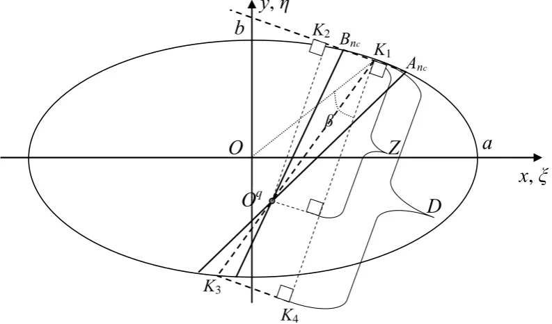
The idea of the presented procedure is based on the integration method for equation of contact mechanics which was proposed by Love (1927), (1929). It based on the integration over the area of thin triangle, which uses the local polar system of coordinates connected with the point of interest Oq
xq,yq
.x
,
ξ
y
,
η
Z
a
b
O
O
qA
nсB
nсK
1K
2K
3D
K
4β
Thus, we need to split crack area into thing triangles by the rays, outgoing from Oq. Rays crossings with crack contour form third sides of triangles – rectifying segments of crack contour. Angle increment for the segmentation rays should be chosen on the base of necessary accuracy, at that corners of crack contour (if exist) are recommended to take into account. The example of the nomenclature for the segmentation triangle
c c n
n qA B
O is shown on Fig. 2. Note, that integral from (2) is changed to the sum of
square integrals for each triangle
c c n
n qA B
O ,nc1..Ncont, where Ncont - is the number of triangles. 1
K is the certain point (e.g. the middle) of c c n
n B
A segment, K2 - point of crossing of
c c n
n B
A line
and normal from Oq. Note, that K2 can be situated at both side outside c c n
n B
A segment, as well as
inside. For the triangle
c c n
n qA B
O its integral can be changed as algebraic sum of two integrals:
c n q c
c n q c
c n c n
q O K B
n K
A O n B
A O
B K sign K
A sign
2 2
) , ( )
,
( 2 2 , (13)
where sign(X,Y) is the certain rule sets the sing of the integral, “+1” if way from contour point X to Y
runs counterclockwise, “-1” – otherwise. For the definiteness purpose integral for OqAncK2 is
considered.
Coordinate system in the triangle is transformed from Cartesian with the center in O point into polar one with the center in Oq, ray OqK2 as polar axis and positive counterclockwise angle Oq direction. This transformation convert singularity of 1/
x
2 y
2 kind into the similar 1/rOq (rOq- the radial coordinate for O A K2c
n q
), but dd transforms into rOqdOqdrOq and Jacobian
determinant reduce the singularity. So, integral part of (2) can be written in the following
“mix-coordinate” form:
q qO
q
c n
q O
Z
O K
A O
dr R
r y x F d
cos
0
2 2
0
1 , 1
2
, (14)
where 1 is the angle An OqK2
c , Z – is the normal length, see Fig. 2. Generally such integral also can’t be solved analytically, so integral expression is replaced by interpolative one-dimension function, which can be integrated. Note, that triangles are quite thing, so we don’t need to use two-dimension interpolation.
Also specificity of near both sides of contour (at K1 and K3 points zone) should be taken into
account. The following polynom-based function, which can be integrated by the known reference analytical recurrent expression, is proposed:
V V
Z z C Z
z C C D
z D Z
z z
F ...
1 1 0
int , (15)
where z – is the distance from c c n
n B
A . Cv(v0..V) coefficients can be also found by the least-squares
method. At that values of expression
Dz D z Z R
r y x
F , 1 2 * 2
along OqK1 segment should be
used. There is an uncertainty of type 0 0
R
R
zz R r z z cos 2 cos 2 1
lim
lim
0 2 2 0 , (16)where is an angle between segment OK1 and normal to
c c n
n B
A .
So, after transformation the final expression for the O A K2
c
n q
integral is following:
. sin 1 sin 1 ln 2 sin 1 sin 1 ln 2 1 cos cos 0 0 2 / 1 1 1 0 0 1 1 0 0 int cos 0 int 0 1 1 2 du D u D Z u C du D u D Z u Z u C du u F d dr r Z F d V v Z v v Z V v v v Z O O O Z O O O K A O q q q q O q q q c n q
(17)Thus the calculation method for the integration part of (2) was developed.
VERIFICATION OF THE METHOD
Integration And Differentiation For The Ellipse Crack
The first and very important set of tests is a comparison of the integration and differentiation results with the well-known data for the elliptical shape. In this chapter results for the full-numerical integration method are also presented for the comparison. At that additional, finer splitting of crack
square near contour was used to take into account features of , because they aren’t considered
analytically in this case. The modeling parameters are following: Nr=N= 40 (number of Oq points by
radial and angular coordinate), Ncont=360, V 10, L=3.
First test was made for Hertz task, obtaining of the integral from (2) for the loading of the ellipse with the law p
x,y p0. The theoretical result is well-known:
22 2 22 2 22
1 ) 1 ( , e e e K e e E a y e e E e K a x e K b p y x o
, (18)
here
a b
a b a
e 2 2 - is the ellipse eccentricity, K(e) and E(e) – are the complete elliptical integrals.
Both methods demonstrated high accuracy. The maximum errors for a/b=1 are 0.1% for numerical approach, 0.0032% – for semianalytical; for a/b=3 errors are 1.5% and 0.02% correspondently.
Second test is the stamp task with loading law p
x,y p0/. The result for the elliptical shape is a constant value. The comparison of theoretical and numerical data is presented in Table 1. Note, that current implementation of presented methods isn’t optimized for such singular stress fields, which is the explanation of such error.Table 1. Calculation results for the stamp task, numerical method
The ellipse geometry Theoretical result, Lurie
(1955)
Result in the center of the ellipse
Maximum error for the whole ellipse square
a= 1, b= 1 29.8696 9.86 0.5%
Next test is the integration and differentiation of (2). Three laws of crack faces opening are
analyzed: U0
x,y 1,
a x y
x
U1 , 1 ,
b y y
x
U2 , 1 . The theoretical results, presented
without material parameters for simplification, are following:
b e E y
x
p0 , 2 ,
2
2
2
1
1 2 1
2 ,
e
e E e e K e a x y
x
p
,
2
2 2
2
1 1
2 ,
e
e K e e
E e b y y
x
p
. Comparison
with our results are shown in Tables 2-3.
Table 2. Calculation results for uniform displacement field U0
Numerical procedure Semianalytical procedure
The ellipse geometry
Theoretical result,
Panasyuk (1968) Result in the
center
Maximum error
Result in the center
Maximum error
a= 1, b= 1 -9.8696 -9.8914 0.3% -9.8691 0.006%
a= 3, b= 1 -6.9978 -7.0149 1.1% -6.9974 0.022%
Table 3. Calculation results for linear displacement fields, U1.and U2, a= 3, b= 1, semianalytical procedure
Values in the points Displacement
function
Maximum of absolute value, Orynyak (1998)
x=-a
(y=-b) 0
x=-a (y=-b)
Maximum error
1
U 8.1091 8.109 10
10
7
-8.109 0.026%
2
U 12.8844 12.884 9
10
9
-12.884 0.009%
So, integration and differentiation procedures demonstrate high accuracy for elliptical shape.
Examples of SIF calculation
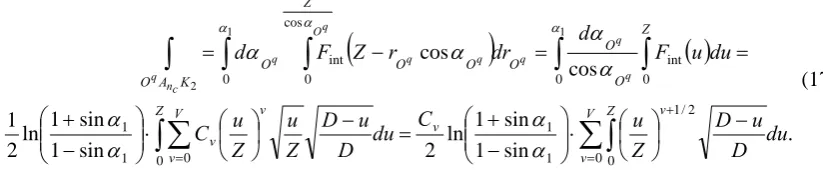
According to the proposed method, SIF for square and semielliptical cracks loaded by uniform stress was obtained. The comparison with Qin and Noda (2003) FEM data for square crack is shown on
Fig. 3. The dimensionless SIF, F1 from Qin and Noda (2003), is presented on the plots. The expression
for the crack face opening for the unit stress is following:
0.1123 0.0086( 2 2)0 x y
H
A
2 2
4 4
0201 . 0 0547
.
0 x y x y
.
The conclusion can be drawn, that accuracy depends on degree of interpolative polynom and one is quite good for L=4. But the question of a result at crack corner zone is still open. The mismatch can be explained by the calculation problem of FEM at such singularity zone. Note, that one of the variants of Qin and Noda (2003) results is closer to our (point “FEM 2” on the plot), but it can be caused by a misprint.
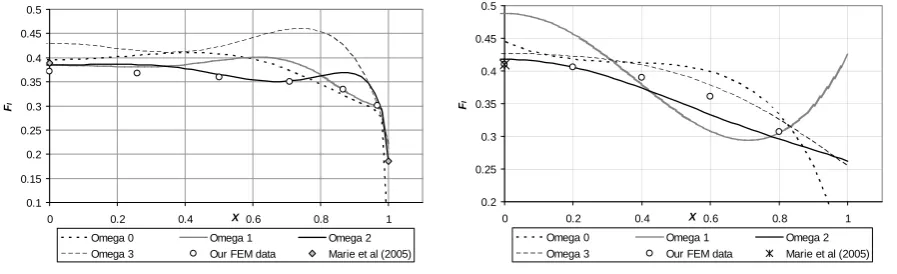
SIF calculation for the semicircular crack of unit radius in the infinite body, having line y=0 as
straight part of contour was performed. For the semielliptical crack form of is a still open question.
Several functions were used in our calculation:
R r b
y
0 1 (point O0, the conditional center of
crack, is (0,0) – the circle center),
2 3
, 2 ,
1 1
R r
O2(0,0.5), O3(0,0.75)). The obtained SIF results were compared with data of Marie et al. (2005) and our
FEM calculations. The best agreement with the FEM data was got for 2. At that proximity of O to the
contour cause certain disagreement of SIF values for nearby points of contour (straight part for O1 and
circular part for O3). The interpolation degree L=4 was used for 0 and L=6 was used for 1,2,3. Using
L=4 for 1,2,3 causes relatively high disagreements and difference in the character of SIF plots.
0 0.1 0.2 0.3 0.4 0.5 0.6 0.7 0.8 0.9
0 0.2 0.4 x/a 0.6 0.8 1
F1
(
K
1 di
m
e
nsi
o
nl
ess)
FEM FEM 2 Degree=2 Degree=4
Figure 3. Result for square crack.
The expression for the crack face opening for the stress 1 MPa and case of best results (2) is
following (odd degrees of x are zero, because of crack symmetry):
6 6
4 2 2
4 5
3 2 4
4
4 2
2 3
2 2
2 0
889 . 6 156 . 0 296
. 3 697
. 2 061 . 22 481
. 8 015 . 1 318 . 27
408 . 0 191
. 6 301 . 16 383
. 0 705 . 4 5 . 0 496 . 0 665 . 0 1 . 0
y x
y x y
x y
y x y
x y
x y
x y
y x y
x y H
A
, (19)
Note, that expression (23) was obtained as first row of M2 matrix, but all other solutions for the
polynomial loading of degrees up to 6th can also be written. The dimensionless SIF parameter
a K
FI I/ 2 obtained for the different is shown on Fig. 4. Results for circular and straight parts
of contour are presented.
0.1 0.15 0.2 0.25 0.3 0.35 0.4 0.45 0.5
0 0.2 0.4 X 0.6 0.8 1
F
I
Omega 0 Omega 1 Omega 2
Omega 3 Our FEM data Marie et al (2005)
0.2 0.25 0.3 0.35 0.4 0.45 0.5
0 0.2 0.4 X0.6 0.8 1
F
I
Omega 0 Omega 1 Omega 2
Omega 3 Our FEM data Marie et al (2005)
A B
CONCLUSION
The original high-effective method of the analytical integration and numerical differentiation of the singular differential-integral equation of flat crack problem was developed. The integration is based on the crack area segmentation with the thing triangles and further analytical integration within triangles square. Then interpolative polynom is built on the base of the integral values through the crack square and Laplace operator can be easily applied to it, so stresses field can be obtained on the base of given crack faces displacement field.
The polynomial statement allows to solve inverse task and to get fields of the crack face opening for the arbitrary polynomial laws of loading. Having displacements of crack fields in the analytical form the stress intensity factor can be easily calculated at any point of crack contour.
The excellent accuracy was shown for the integration and differentiation procedures. Obtained SIF results for the square and semielliptical cracks show good correspondence with FEM data, at that new
SIF data for the polynomial loading laws up to 6th degree were obtained. The importance of the polynom
degree and shape function for the calculation accuracy was demonstrated.
REFERENCES
Orynyak, I.V., Borodii, M.V. and Torop, V.M. (1994). “Approximate Construction of a Weight Function for Quarter-elliptical, Semi-elliptical and Elliptical Cracks Subjected to Normal stresses,”
Engineering Fracture Mechanics, 49(1), 143-151.
VERLIFE (2008). Unified Procedure for Lifetime Assessment of Components and Piping in WWER
NPPs, “VERLIFE” Version 2008, Project co-funded by the European Commission under the Euratom Research and Training Programme on Nuclear Energy within the Sixth Framework Programme (2002-2006).
Panasyuk, V.V. (1988). Fracture Mechanics and Strength of Materials. Vol. 2. Stress Intensity Factors
for the Bodies With Cracks (in Russian), Naukova Dumka, Kyiv, Ukraine (former USSR).
Panasyuk, V.V. (1968). Ultimate Equilibrium of the Brittle Bodies with cracks (in Russian language),
Naukova Dumka, Kyiv, Ukraine (former USSR).
Stadnik, M.M. and Gorbachevskiy, I.Ya. (1981). “Limit Equilibrium of Body With a Flat Triangular
Crack,” Prickladnaya Mechanika, 17(7), 101-105.
Qin, T.Y. and Noda, N.A. (2003). “Stress Intensity Factors of a Rectangular Crack Meeting a Bimaterial Interface,” International Journal of Solids and Structures, 40, 2473–2486.
Tang, R.J. and Qin, T.Y. (1993). “Method of Hypersingular Integral Equations in Three-dimensional
Fracture Mechanics,” Acta Mechanica Sinica, 25, 665–675.
Love, A.E.H. (1927). A Treatise on the Mathematical Theory of Elasticity, 4th edition, Cambridge
University Press.
Love, A.E.H. (1929). “The Stress Produced in a Semi-infinite Solid by Pressure on Part of the Boundary,”
Philosophical Transactions of the Royal Society, London,A228:377.
Lurie, A.I. (1955). Spatial Problems of Elasticity Theory (in Russian), State Publishing House of
Scientific-Technical Literature, Moscow, Russia (former USSR).
Orynyak, I.V. (1998). “Method of Translation a Mode I Elliptic Crack in an Infinite Body. Part I.
Polynomial Loading,” International Journal of Solids and Structures, 35, 3029-3042
Marie, S., Me´nager, Y. and Chapuliot, S. (2005). “Stress Intensity Factors for Underclad and Through clad Defects in a Reactor Pressure Vessel Submitted to a Pressurised Thermal Shock,”