ABSTRACT
ABBEY, RALPH WALTER. Stochastic Clustering: Visualization and Application. (Under the direction of Dr. Carl D. Meyer.)
Data clustering is an important task in the field of data mining. In many cases clustering is used as an exploratory tool to better understand data. However, one difficulty in clustering is determining the quality of a given clustering result. While many clustering algorithms exist, we focus on a recently developed algorithm: stochastic clustering. We show how the results of the stochastic clustering can be visualized, and how this visualization indicates the quality of the clustering result.
One key step in stochastic clustering is to convert a nearly uncoupled similarity matrix into a doubly stochastic matrix. We propose an alternate iterative method to the commonly used Sinkhorn-Knopp algorithm, and provide error bounds in the limit. Additionally we develop stricter bounds than previously determined, that show the conversion to doubly stochastic form neither creates nor destroys the nearly uncoupled property.
© Copyright 2014 by Ralph Walter Abbey
Stochastic Clustering: Visualization and Application
by
Ralph Walter Abbey
A dissertation submitted to the Graduate Faculty of North Carolina State University
in partial fulfillment of the requirements for the Degree of
Doctor of Philosophy
Mathematics
Raleigh, North Carolina 2014
APPROVED BY:
Dr. Ilse Ipsen Dr. Rada Chirkova
Dr. Ernie Stitzinger Dr. Carl D. Meyer
DEDICATION
BIOGRAPHY
ACKNOWLEDGEMENTS
I’d like to acknowledge my wife, my family, and my friends for their support, especially Zack Kenz and Miriam Diller during the thesis editing process. I’d like to thank the members on my committee for making time in their busy schedules for me. I’d like to thank Dr. Meyer for having me as a student and his advising and mentoring effort. I’m especially grateful to Dr. Meyer for his REU back in 2007 in which he introduced me to world of data mining.
TABLE OF CONTENTS
LIST OF TABLES . . . vii
LIST OF FIGURES . . . viii
CHAPTER 1 Introduction . . . 1
1.1 Data Clustering . . . 1
1.1.1 Motivating Example . . . 2
1.2 Data Visualization . . . 3
1.3 Similarity Graphs and Matrices . . . 3
1.4 Stochastic Consensus Clustering . . . 5
1.4.1 Organization and Goals . . . 6
CHAPTER 2 Stochastic Consensus Clustering Background . . . 8
2.1 Notation and Terminology . . . 8
2.1.1 Eigenvalue Notation . . . 9
2.1.2 Non-Zero Structure of a Matrix . . . 9
2.1.3 Nearly Uncoupled Matrices . . . 13
2.1.4 Stochastic Matrices and the Simon-Ando Theory . . . 14
2.1.5 Stochastic Complementation . . . 15
2.2 The Existence of a Doubly Stochastic Matrix, P . . . 19
CHAPTER 3 Matrix Scaling . . . 20
3.1 Properties of a Doubly Stochastic Matrix,P . . . 20
3.1.1 The ‘Uncoupling Measure’ and the ‘Row Uncoupling Measure’ . . . 23
3.2 Algorithms for Obtaining a Doubly Stochastic Matrix,P . . . 25
3.2.1 Sinkhorn-Knopp Algorithm . . . 25
3.3 Alternative to the Sinkhorn-Knopp . . . 27
3.3.1 Simultaneous Scaling . . . 31
3.4 Rate of Asymptotic Convergence . . . 33
CHAPTER 4 Initializations and Visualizations . . . 36
4.1 Visualization of the Evolving Markov Chain . . . 38
4.2 Stochastic Clustering Initialization Concerns . . . 42
4.2.1 Initial Probability Vectors Leading to No Solution . . . 42
4.2.2 Initial Probability Vectors Leading to Misleading Solutions . . . 43
4.3 Using Multiple Initial Probability Vectors, and Extending Visualizations . . . . 45
CHAPTER 5 Experimental Setup . . . 48
5.1 K-means . . . 48
5.1.1 K-means Initializations . . . 49
5.1.2 K-means Variants . . . 51
5.2.1 Similarities Between Spectral Clustering and Stochastic Consensus
Clus-tering . . . 53
5.3 Experimental Setup . . . 53
CHAPTER 6 Experimental Results and Discussion . . . 55
6.1 Clustering Data Sets with Known Cluster Structure . . . 56
6.1.1 Breast Cancer Data Set [50] . . . 56
6.1.2 Medlars, Cranfield, Cisi (MCC) Data Set ([22] pg. 74) . . . 58
6.1.3 Digits Data Set from the MNIST Database [44] . . . 62
6.1.4 Small Practice Data Sets . . . 66
6.2 Exploring Data Sets Using Visualization . . . 66
6.2.1 Spoken Letters Data Set [25] . . . 67
6.2.2 Steel Faults Data Set as found on the UCI repository[7] . . . 69
6.2.3 Million Song Data Set [10] . . . 70
CHAPTER 7 Discussion and Concluding Remarks . . . 74
7.1 Conclusion . . . 75
7.1.1 Contributions . . . 75
7.1.2 Future Research . . . 76
REFERENCES . . . 77
APPENDICES . . . 83
APPENDIX A Stochastic Clustering Matlab GUI . . . 84
APPENDIX B Distributed Memory Stochastic Clustering . . . 89
B.1 Distributed Similarity Construction . . . 89
LIST OF TABLES
Table 6.1 Accuracy and timing results for the breast cancer data set. . . 58 Table 6.2 Accuracy and timing results for the MCC data set. . . 61 Table 6.3 Accuracy and timing results for the digits data set. . . 65 Table 6.4 Accuracy of the stochastic consensus clustering algorithm on small
LIST OF FIGURES
Figure 2.1 An example of the computation for a stochastic complement (Wessell [86], pg. 16). The equation for the stochastic complement C22 whenP is
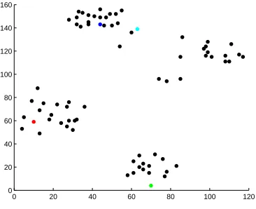
a matrix with four diagonal blocks. . . 15 Figure 4.1 Ruspini data [left] and the Ruspini data separated into four clusters [right] 37 Figure 4.2 Plots of s4, the 4th evolution of the Markov chain, on the Ruspini data.
[Left] is a plot without coloring according to separating at the k−1 largest gaps, while [Right] shows coloring by determined cluster. . . 39 Figure 4.3 Plots of s0 [Left] and s1 [Right] on the Ruspini data. . . 40
Figure 4.4 Plots of s2 [Left] and s3 [Right] on the Ruspini data. . . 40
Figure 4.5 Plots of s19 [Left] and s49 [Right] on the Ruspini data. The probability
vector is converging to the uniform probability vector. . . 41 Figure 4.6 Plots of s0 [Left] and s1 [Right] on the Ruspini data. . . 44
Figure 4.7 Plots of s2 [Left] and s7 [Right] on the Ruspini data. In s2 we see that
two of the clusters have reached approximately the same value before the short-run dynamics are witnessed. In s7 we see another problem that if
too many steps are taken some of the differences can become meaningless. 45 Figure 4.8 Plots of s0 versus r0 [Left] ands1 versusr1 [Right] on the Ruspini data. 46
Figure 4.9 Plots ofs2versusr2 [Left] ands2versusr2colored after clustering [Right]
on the Ruspini data. . . 47 Figure 5.1 Example of the random initialization on the Ruspini data set. . . 50 Figure 5.2 Example of the Forgy initialization on the Ruspini data set. Black data
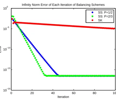
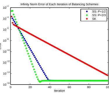
points do not yet belong to any cluster. . . 50 Figure 6.1 Plot of the error per iteration of various balancing schemes on the breast
cancer data set. . . 56 Figure 6.2 Absolute (left) and relative (right) error between double and
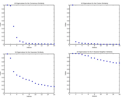
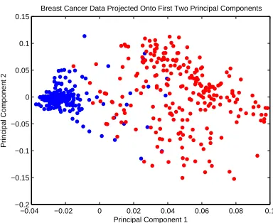
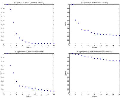
quadru-ple precision of the simultaneous scaling on the breast cancer data set, computed in quadruple precision. . . 57 Figure 6.3 Eigenvalue plots for similarity matrices on the breast cancer data set. . 58 Figure 6.4 Visualization of the clustered data using the consensus similarity matrix
on the breast cancer data set. Indices are unordered (left) and ordered by true cluster (right). . . 59 Figure 6.5 Visualization of the raw breast cancer data using PCA. The observations
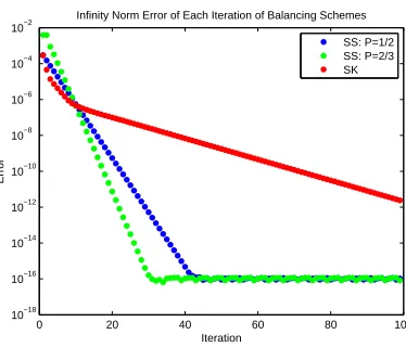
have been colored by cluster membership. . . 59 Figure 6.6 Plot of the error per iteration of various balancing schemes on the MCC
data set. . . 60 Figure 6.7 Absolute (left) and relative (right) error between double and quadruple
Figure 6.9 Visualization of the clustered data using the consensus similarity matrix on the MCC data set. Indices are unordered (left) and ordered by true
cluster (right). . . 63
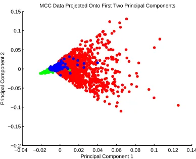
Figure 6.10 Visualization of the raw MCC data using PCA. The observations have been colored by cluster membership. . . 63
Figure 6.11 Plot of the error per iteration of various balancing schemes on the digits data set. . . 64
Figure 6.12 Absolute (left) and relative (right) error between double and quadruple precision of the simultaneous scaling on the Digits data set, computed in quadruple precision. . . 64
Figure 6.13 Eigenvalue plots for similarity matrices on the digits data set. . . 65
Figure 6.14 Visualization of the clustered data using the consensus similarity matrix on the digits data set. Indices are unordered (left) and ordered by true cluster (right). . . 66
Figure 6.15 Visualization of the raw Digits data using PCA. The observations have been colored by cluster membership. . . 67
Figure 6.16 Visualization of the data using the consensus similarity matrix on the letters data set. . . 68
Figure 6.17 Visualization of the manually clustered data using the consensus similar-ity matrix on the letters data set. . . 69
Figure 6.18 Visualization of index by probability plots using stochastic consensus clustering on the steel faults data set, ordered by steel fault type. . . 70
Figure 6.19 Visualization of probability by index plot, using stochastic consensus clustering on the Million Song Data Set. We keep the y axis the same in each plot to illustrate the converging Markov chain. . . 71
Figure 6.20 Visualization of probability by probability plots, using stochastic con-sensus clustering on the Million Song Data Set. The x and y axis are rescaled for each plot so the points are more noticeably distinct. . . 72
Figure A.1 First call the GUI using the command SCA in Matlab. . . 84
Figure A.2 This is the interface the user first sees. . . 85
Figure A.3 Type in the .mat file, and click ‘balance matrix’. Then click ‘initialize’ and then click ‘plot’. . . 85
Figure A.4 The first plot that is created by the GUI. . . 86
Figure A.5 By clicking ‘next’, we get this plot. . . 86
Figure A.6 By clicking ‘next’ again, we get this plot. . . 86
Figure A.7 Input 3 into ‘k=’ and then click ‘cluster’. . . 87
Figure A.8 Click ‘auto label’ to label the indices automatically. . . 87
Figure A.9 The previous step 2 plot now clustered. . . 87
Figure A.10 Instead we want to import a known clustering. Click ‘use labels’ type in the .mat file name, and click ‘import’. . . 88
CHAPTER
1
Introduction
1.1
Data Clustering
Data clustering, or just clustering, is the task of segmenting a set of observations into groups, such that similar observation are in the same groups, while dissimilar observations are in dif-ferent groups. The set of observations we call the data set, and the groups we call clusters. The task of clustering can be a goal in itself, or part of a larger data mining and knowledge discovery process, where clustering is used for summarization, compression, or in finding nearest neighbors ([79] pg. 489).
The SEMMA model of data mining applications, which stands for Sample, Explore, Modify, Model, and Assess, places clustering in the Explore stage [6]. This is because clustering is inherently an exploratory task, in which a user seeks to gain new insight into the data.
Clustering is not just a task of academic curiosity, but also of interest to business and in-dustry, as illustrated in commercial products such as SAS®Enterprise Miner[70] and Radoop [65] which include tools for clustering. Clustering is useful in many computational fields such as pattern recognition, information retrieval, machine learning, classification, and bio-informatics. Due to the shared interest in both academic and business communities, as well as the wide variety of fields in which it is used, clustering is a broad topic with many algorithms, both specialized and generic. One reason for the large quantity of algorithms is summarized nicely in the following statement.
Theorem 1.1.1. ([41] pg. xiv)
solving all problems in a given class of problems.
Additionally, as clustering is fundamentally an exploratory task, different methods can pro-vide different results, all of which could be meaningful. While there may be many good clustering results, and many good clustering methods, we should be careful to not fall into the trap of thinking that all results and all methods are equally valid. While there may be multiple ‘correct’ answers in clustering, there are still wrong answers: grouping observations that are dissimilar together.
1.1.1 Motivating Example
Let us consider an industry application of clustering as a motivating example for our goals in this thesis. We consider a data analyst working for a major credit card company who wishes to create a model to predict which customers are most likely to churn; that is, to cancel their card. By creating a model that accurately predicts which customers may churn, the analyst enables the credit card company to offer special promotions to keep customers from leaving.
The data analyst uses clustering as an initial step to segment the customers into groups. She then creates a different classification model for each group separately, thereby improving the overall classification (application paraphrased from [20]). Ultimately the analyst helps the credit card company retain customers and increase profit.
Clustering is an important part of the predictive modeling process. A good clustering al-gorithm will group similar customers together, which can improve the predictive methods that the data analyst uses. The data analyst in our scenario wants several things from a clustering algorithm. Primarily, she wants the algorithm to work well at the clustering task: segmenting the customers into groups based on of similarities. She also knows that one specific clustering algorithm may not perform well in all cases. Thus her second desire is for a way to validate that the clustering algorithm performed as desired.
1.2
Data Visualization
The exploratory task of clustering is also highly tied to data visualization. Data visualization is the act of presenting representations of the data that a user can see. Visualization supports the human ability to look for patterns and relationships in the data ([26] pg. 21). It naturally occurs during the Explore phase of the SEMMA model, just as clustering does. Because there is no single clustering algorithm that we can turn to in all situations, having good cluster visualization methods can help indicate to a user whether a given clustering method is useful for a particular application.
Data visualization is used in many fields of science, and it includes many techniques that are specialized for a given purpose or data set (e.g. [30], and as can be seen in places such as [34] [60]). In this thesis we focus specifically on visualization of points inRn without regard to a specific field or underlying structure. From our motivating example, we specifically want to investigate how visualization can aid in cluster validation.
Many generic methods have been proposed to visualize data, especially high dimensional data, including by using projections [52] [5] [31] [32] [3] [80], plotting parallel coordinates [88], using interactive methods [14], and using many other methods on which entire books have been written [26].
Clustering can aid in the visualization process as well, due to the fact that the act of clus-tering collects similar observations together, based off of patterns in the data. The data can be reorganized according to the determined clustering, thus allowing a more intuitive presentation of the data. In addition to the plethora of visualization methods for data, many methods have been proposed that use clustering in the visualization process [19] [2] [15] [83] [66]. Finally, some visualization methods, such as those in the Gephi software package [8], are designed for specific structures of data.
1.3
Similarity Graphs and Matrices
In many traditional clustering formulations a dataset of n observations and m numerical at-tributes is represented as anm×nmatrix,M. An example of this formulation can be found in organizing textual documents, in which the attributes are the words and thusMij would be the number of times that word iappears in document j. Many of the aforementioned visualization techniques also use this representation in generating the visual representations of the data. An alternative way to represent the data is through the creation of similarity matrices.
to have low weight.
Given a set of data pointsxi∈Rnand a measure of similarity, a similarity graph is defined where each vertex vi represents the data point xi, and the edge between vi and vj has weight Sij. IfSij = 0 then there is no edge betweenvi and vj.
A similarity matrixSis a symmetric matrix in whichSij is the similarity betweenxi andxj. This matrix is the adjacency matrix of the similarity graph. We will continue our discussions in terms of the similarity matrix, though all of these ideas can be traced back to the graphs that the similarity matrix describes.
We introduce a few measures of similarity here which will be used in later portions of the thesis.
Gaussian kernel [42] similarity - The Gaussian kernel similarity matrix is used in spectral clustering [84]. This similarity matrix includes a user determined parameter,σ >0 which is used to control the spread of the similarity values.
Sij =e
−kxi−xjk
2 2
σij
Cosine similarity - The cosine similarity is often used with word document sets ([79] pg. 75).
Sij =
xTi xj kxik2kxjk2
Shared K-nearest neighbor similarity [37] - The shared k-nearest neighbor similarity de-fines the similarity between two observations by the number of ‘neighbors’ they share. For each observation and a given distance metric, first construct the list of theK nearest neighbors. Sij is the size of the intersection of the nearest neighbor lists for observation iand observation j. In [37] nearest refers to Euclidean distance, but this concept can be generalized to any distance measure.
Consensus similarity - The consensus similarity matrix is different from the previous three similarity matrices in that it requires the observations to have previously been clustered by multiple algorithms, or multiple times by an algorithm with random initializations. The consensus similarity, as the name implies, tries creates a similarity in which the goal is to find a consensus between the previously-run clustering methods.
a(ijk) =
1 : if observationsi andj were clustered together 0 : if observationiand j were not clustered together Definition 1.3.1. ([86] pg. 5)
If {A(1), A(2), . . . , A(r)} is a collection of adjacency matrices created from clusterings of the same data set, then the sum of these matrices
S =A(1)+A(2)+· · ·+A(r)
is called the consensus similarity matrixor the consensus matrix.
From our earlier discussion of clustering algorithms we know that many different clustering results can be obtained from a given data set. It is a natural desire, then, to want to find some agreement between different clustering results. The consensus similarity matrix is of particular interest due the fact that partitioning it acts as meta-clustering: we use previously determined clustering results to generate a graph we then seek to partition.
One recently developed method using the consensus similarity matrix is the stochastic con-sensus clustering algorithm. It is this method that we consider in this thesis.
1.4
Stochastic Consensus Clustering
The stochastic consensus clustering algorithm is shown below:
Algorithm 1.4.1. Stochastic Consensus Clustering Algorithm [86]
Input: N observations xi ∈Rm.
1. Create the consensus similarity matrixS using a clustering consensus of the user’s choice
2. Use matrix balancing to convert S into a doubly stochastic symmetric matrixP.
3. Compute eigenvalues of P. Sort the eigenvalues of P in descending order and find the
largest difference between successive eigenvalues. Letkbe the number of eigenvalues before
the largest difference.
5. Track the evolution sTt =sTt−1P. After each iteration, sort the elements of sTt and then
separate the elements into k clusters by dividing the sorted list at the k−1 largest gaps.
When this clustering remains the same for a user-defined number of iterations, the final
clusters are determined.
Output: Clusters C1, . . . , Ck.
The stochastic consensus clustering algorithm (Wessell [86]) is a recently created algorithm that uses the consensus similarity matrix to perform data clustering. One of the original motiva-tions is that stochastic consensus clustering acts as a way to create consensus among multiple clusterings, thus boosting user confidence in the final confidence of the result - a key factor in our motivating example. The second motivation is that the stochastic consensus clustering algorithm provides the user with k, the number of clusters, as opposed to requiring k as an input.
Other methods for determining k include the statistical technique called the gap statistic
[82]; spectral clustering [84], which is another graph-based method; methods that look at the percentage of variance explained by different numbers of clusters [38] [81]; using cross-validation over multiple choices fork [78]; and optimizing a given metric over multiple choices ofk [46].
1.4.1 Organization and Goals
All proofs in this thesis are original; non-original theorems are cited without proof. We will often use the phrase ‘stochastic clustering algorithm’ or ‘stochastic consensus clustering algorithm.’ The latter phrase refers specifically to the formulation in Algorithm 1.4.1, whereas the former is a more general case in which any similarity matrix is used (not just the consensus similarity - see step 1). This thesis investigates both the general and the specific cases.
In our motivating example the data analyst wants two main things: for her clustering method of choice to work well, and to be able to verify that it works well. The traditional method for showing a clustering method works well for a given application is to use data with known clusters and to show that the clustering obtains the known result.
We have three main goals in this thesis.
We wish to show that the stochastic clustering algorithm can generally perform well, which is mainly an experimental endeavor. We will do this by comparing the stochastic clustering algorithm to spectral clustering, a popular similarity matrix-based clustering method. We com-pare these two methods on several data sets that have a wide range in number of observations as well as a wide range in application areas.
which the stochastic clustering algorithm can be improved. We explore three of these questions: 1) Is there another similarity measure for which stochastic clustering will work? 2) Can the Sinkhorn-Knopp algorithm be replaced by one instance of row and column scaling? 3) Can we improve the theoretical bounds relating consensus matrix,S, to its doubly stochastic form, P? We address 1) experimentally and 2) by proposing a faster balancing algorithm to cut the potentially long convergence times for the Sinkhorn-Knopp.
Finally, we wish to provide a way for a user to validate the clustering output. We propose a method for visualizing the output of the stochastic clustering algorithm. We claim that this visualization allows a user to visually validate how the clustering is performing without having to decipher tables of numbers, or to inspect specific clustering results.
We organize this thesis as follows. In Chapter 2 of this thesis we focus on the theoretical background for the stochastic clustering algorithm. This theoretical background is necessary for our goals of improving the algorithm, as well as visualization. In Chapter 3 we show im-provements for the bounds relating the consensus similarity matrix,S, to the doubly stochastic matrix, P. In addition, we provide a new algorithm that we argue will convert S to P faster than currently used methods, when appropriate prerequisites are met.
In Chapter 4 we introduce a method of visualizing the data and clustering from the stochas-tic consensus clustering method. We argue that through visualization a user can both validate the quality of clustering as well as improve upon the standard results of the stochastic clus-tering algorithm. We also discuss the initialization of the Markov chain related to step 4 of the stochastic clustering algorithm. We expand previous work on the theoretical issues that can cause poor initializations. Through the use of visualization we argue that it is possible to understand when a poor initialization has been encountered.
We discuss experimental setup and results in Chapters 5 and 6 respectively. In Chapter 6 we show experimentally that stochastic stochastic consensus clustering performs well in comparison to spectral clustering on several different datasets. We show that the consensus similarity matrix is the appropriate similarity matrix on which to use the stochastic clustering. We also show how visualization can provide valuable insight for the clustering process and validation.
CHAPTER
2
Stochastic Consensus Clustering Background
The stochastic clustering algorithm investigated in this thesis is based upon the variable ag-gregation work of Herbert Simon and Albert Ando [74]. In Section 2.1 we define notation and terminology that are used in this thesis, as well as provide relevant theorems for the introduced terminology. In Section 2.1.4 we give a brief overview of the Simon-Ando theory, and we explain how we use its results in the stochastic clustering algorithm. We finish this chapter by showing that we can generate an appropriate matrix for the Simon-Ando theory from the similarity matrices discussed in Chapter 1.
2.1
Notation and Terminology
We start with general notation, after which we break notation down into the topic areas of eigenvalue notation and notation which deals with matrix structure.
Definition 2.1.1. (Meyer [54], pg. 663)
If A ∈ Rm×n such that a
ij > 0 for all elements of A, then we say that A is a positive
matrix, which we denote byA >0.
Definition 2.1.2. (Meyer [54], pg. 670)
If A∈Rm×n such thataij ≥0 for all elements ofA, then we say thatA is a nonnegative
matrix, which we denote byA≥0.
2.1.1 Eigenvalue Notation
Eigenvalues are used in this thesis during the discussion of convergence for some of the algo-rithms later presented. To avoid confusion as to which matrix to which an eigenvalue belongs, we useλi(A) to denote thatλi is an eigenvalue ofA.
It is useful to be able to order the eigenvalues of a matrix. For anyn×nmatrixAwe can order the eigenvalues by the magnitude of the modulus such that |λ1(A)| ≥ |λ2(A)| ≥ · · · ≥ |λn(A)|.
If we know that A has all real eigenvalues then we can also order by the eigenvalues such thatλ1(A)≥λ2(A)≥ · · · ≥λn(A).
We use both orderings in this thesis, and as such the presence of the absolute value symbol, or lack thereof, will indicate which ordering is being used.
Definition 2.1.3. (Meyer [54], pg. 497)
The spectral radius of a n×n matrix A, ρ(A), is the maximum of the modulus of all
eigenvalues of A. That is ρ(A) = maxi|λi(A)|.
2.1.2 Non-Zero Structure of a Matrix
We now define the termsfully indecomposable,total support,irreducible, andprimitive, all of which deal with the structure of a matrix, or the locations of zeros and non-zeros in a matrix. We also provide some additional theorems that relate these concepts to each other. These terms are used in the theorems that relate to the Simon-Ando theory, and also to show how the stochastic clustering algorithm satisfies necessary assumptions.
Some concepts have multiple terms associated with them in the literature. For example completely indecomposable is used in [45], while in many other sources the term used is fully indecomposable [40] [13] [9]. The term indecomposable has also been used to have the same meaning as irreducible[21].
Definition 2.1.4. (Meyer [54], pg. 671)
An n×n nonnegative matrixA is said to bereducible if there exists a permutation matrix
Q such that
QTAQ=
"
X Y
0 Z
#
where X andZ are both square. If no such permutation exists then Ais said to beirreducible.
Definition 2.1.5. (Meyer [54], pg. 674)
An irreducible matrix A is said to be a primitive matrix if λ1(A) =ρ(A), and |λi(A)|<
|λ1(A)| for i6= 1.
Example 2.1.6. (If A is an irreducible matrix, thenA is not necessarily primitive.)
A=
"
0 1 1 0
#
It is clear that A is irreducible. However A has the eigenvalues of -1 and 1, and thus A is not
primitive because |λ2(A)| 6<|λ1(A)|.
Theorem 2.1.7. (Meyer [54] pg. 678)
If A is an irreducible matrix, thenA is primitive if and only if there exists an integer k >0
such that Ak>0.
Example 2.1.6 also illustrates Theorem 2.1.7, as A2 =I. Therefore there is no k such that Ak>0.
Theorem 2.1.8. (Plemmons [9], pg. 34)
If A is an irreducible matrix with a positive trace, then A is primitive.
It is worth noting that the converse of Theorem 2.1.8 is not necessarily true: ifAis primitive, it is not generally required thatAhave a positive trace. We illustrate this in Example 2.1.9. In the case of 2×2 matrices it is true thatAhas a positive trace if A is primitive.
Example 2.1.9.
A=
0 1 1 1 0 1 1 1 0
, A
2 =
2 1 1 1 2 1 1 1 2
In this case A does not have a positive trace, but A is primitive because A2 >0.
Several proofs that we discuss later, by Sinkhorn and Knopp, Brualdi, and also Ruiz, require a generalization of the concept of irreducible.
Definition 2.1.10. (Minc [55] pg. 82)
An n×nnonnegative matrix A is said to befully indecomposable if there are no
permu-tation matrices Q1 and Q2 such that
Q1AQ2 = "
X Y
0 Z
#
where X and Z are both square.
Example 2.1.11. (Irreducible does not imply fully indecomposable)
Q1 and Q2 are the only 2×2 permutation matrices
Q1 = "
1 0 0 1
#
, Q2 = "
0 1 1 0
#
.
If A is
A=
"
0 1 1 1
#
then A is irreducible as neither QT1AQ1 nor QT2AQ2 are reducible. However, A is not fully
indecomposable, as seen by computing Q2AQ1.
Q2AQ1 = "
1 1 0 1
#
In order to more fully relate irreducible and fully indecomposable, we need the concept of total support.
Definition 2.1.12. (Sinkhorn and Knopp [75] pg. 343)
Given an n×nreal matrixA, and a permutation,σ, of the numbers1,2, . . . , n, the sequence
of elementsa1σ(1), a2σ(2), . . . , anσ(n) is thediagonalofA corresponding toσ. Ifσ is the identity
permutation, then the diagonal is called the main diagonal.
Definition 2.1.13. (Sinkhorn and Knopp [75] pg. 343))
If A is an n×n nonnegative matrix, Ais said to have total support if A6= 0 and if every
positive element ofA lies on a positive diagonal (where a1σ(1), a2σ(2), . . . , anσ(n)>0is one such
diagonal).
As much of the discussion in this thesis focuses on symmetric matrices, especially with a positive main diagonal, we relate these types of matrices to the concept of total support. Lemma 2.1.14. If A is a nonnegative symmetric matrix with a positive main diagonal, then
A has total support.
Proof. To prove this, we need to show that every positive element lies on a positive diagonal.
Foraij >0 we defineσij to be the permutation whereσ(i) =j,σ(j) =i, andσ(k) =kfor all k6=i, j. BecauseAhas a positive main diagonal we know that ifk6=i, j thenakσ(k)=akk>0.
Since Ais symmetric, ifaij >0, thenaiσ(i) =aij =aji=ajσ(j) >0. Thusaij lies on a positive diagonal.
Lemma 2.1.15. (Minc [55] pg. 83)
Every positive entry of a fully indecomposable matrix lies on a positive diagonal.
Theorem 2.1.16. (Csima and Datta [18] pg. 149)
Let A be an irreducible symmetric matrix with total support. Then either A is fully
inde-composable or else there exists a permutation matrix Qsuch that
QAQT =
"
0 B
BT 0
#
where B is fully indecomposable.
It is also noted that if Ais a fully indecomposable matrix, then Ais also primitive [12] [39] [9][55]. A proof can be found in [45].
Theorem 2.1.17. (Lewin [45] pg. 756)
If A is a fully indecomposable nonnegative matrix then An−1>0.
We synthesize the independent theorems and definitions into one theorem that relates the concepts of irreducible, primitive, total support, and fully indecomposable. This is especially useful as the similarity matrices used in this thesis are symmetric.
Theorem 2.1.18. A symmetric matrix Ais fully indecomposable if and only ifAis irreducible, primitive, and has total support.
Proof. (⇒) AssumeAis fully indecomposable. ThenAis irreducible (Definition 2.1.10), Ahas
total support (Lemma 2.1.15), andA is primitive (Theorem 2.1.17).
(⇐) AssumeAis irreducible, primitive, and has total support. Theorem 2.1.16 ensures that eitherA is fully indecomposable or Ahas the form
QAQT =
"
0 B
BT 0
#
,
where B is fully indecomposable and Q is a permutation matrix. Since A is primitive, any symmetric permutation ofA must be primitive. ThereforeA is fully indecomposable.
We note that whenAis not symmetric, the (⇒) direction is still true, but the (⇐) direction does not hold. We provide a counter example in Example 2.1.19.
A=
0 1 1 0 1 1 1 0 0
We see that A has total support by considering the diagonal formed by (a31, a22, a13) and the
diagonal formed by (a31,a23,a12). Each positive element ofAlies on one of these two diagonals,
and each of these diagonals is made up of strictly positive elements.
There exists no permutation matrix Q such that QAQT is reducible, and we also see that
A is primitive because A3 > 0. Thus we know that A is irreducible, primitive, and has total
support. Given Q1 andQ2
Q1 =
0 0 1 0 1 0 1 0 0
and Q2 =
1 0 0 0 1 0 0 0 1
,
then
Q1AQ2 =
1 0 0 0 1 1 0 1 1
.
The computation Q1AQ2 shows thatA is not fully indecomposable, which finishes the
coun-terexample.
2.1.3 Nearly Uncoupled Matrices
The Simon-Ando theory, and thus the stochastic clustering algorithm, relies on the concept of nearly uncoupled matrices.
Definition 2.1.20. (Wessell [87] pg. 1216)
The n×nmatrix A is called uncoupled if it can be symmetrically permuted to the form
QAQT =
A?11 0 . . . 0 0 A?
22 . . . 0
..
. ... . .. ...
0 0 . . . A?kk
where the diagonal blocksA?ii are square with size ni×ni, andn1+n2+· · ·+nk=n.
A matrix that cannot be permuted to the form in Definition 2.1.20 is not uncoupled. Theorem 2.1.21. (Wessel [86] pg. 13)
If A is a matrix that is ‘very close’ to an uncoupled matrix, then we say that A is nearly uncoupled. We give a definition for stochastic matrices in 2.1.5, and a more general definition in Chapter 3.
If the similarity matrix used as input to Algorithm 1.4.1 is nearly uncoupled then we can use the Simon-Ando theory to find clusters. We examine this theory in the next section.
2.1.4 Stochastic Matrices and the Simon-Ando Theory
Definition 2.1.22. (Meyer [54], pg. 687) A stochastic matrixis a nonnegative matrixPn×n
in which each row sum is equal to 1.
In some cases a matrix may be referred to as either ‘row stochastic’ or ‘column stochastic’ as an indication of the rows or columns summing to 1 respectively. A matrix whose row sums and column sums both equal 1 is said to be doubly stochastic.
We call a nonnegative vector πT a probability row vector ifkπTk1 = 1. IfP is a stochastic matrix andπ0T is a probability row vector then we can consider the evolution equation
πTt =πtT−1P, (2.1)
where each πTt will also be a probability row vector.
Definition 2.1.23. (Wessell [86], pg 14) The row vectorπT is a stationary distribution vector
of the stochastic matrixP if it satisfies the equations
πT = πTP πT ≥ 0 πTe = 1
where e is the vector of all ones.
IfP is primitive then we are guaranteed that a stationary distribution vectorπT exists, and
πT = lim t→∞π
T
0P
for any initial probability row vectorπT0.
given a known long-term behavior of the evolution equation, the goal is to find clusters by observing the short-run and middle-run behavior.
The stochastic clustering method requires that the input similarity matrix be converted to a doubly stochastic matrix. We continue this chapter with the assumption that such a conversation is possible. We discuss the details of this conversion at the end of this chapter, and in Chapter 3 of this thesis.
Simon and Ando argued that if P is primitive and nearly uncoupled, then πtT will go through several distinct stages before approaching the limit as a stationary distribution vector. To formally define these stages, we next define the stochastic complement.
2.1.5 Stochastic Complementation
Definition 2.1.24. (Meyer [53], pg. 2) Let P be an n×n irreducible stochastic matrix with the structure P =
P11 P12 . . . P1k P21 P22 . . . P2k
..
. ... . .. ...
Pk1 Pk2 . . . Pkk
in which all diagonal blocks are square. Then eachPiihas a stochastic complement in P defined
by
Cii=Pii+Pi?(I−Pi)−1P?i,
where Pi is the matrix obtained by deleting the ith row and ith column of blocks from P. Pi? is
the ith row of blocks of P excluding Pii, and P?i is the ith column of blocks also excluding Pii.
P =
P11 P12 P13 P14
P21 P22 P23 P24
P31 P32 P33 P34
P41 P42 P43 P44
C22 = P22+P2?(I−P2)−1P?2
C22 = P22+
P21 P23 P24
I−P11 −P13 −P14
−P31 I −P33 −P34
−P41 −P43 I−P44
−1
P12 P32 P42
Theorem 2.1.25. (Meyer [53], pg. 22) For ann×n irreducible stochastic matrix of the form P =
P11 P12 . . . P1k P21 P22 . . . P2k
..
. ... . .. ...
Pk1 Pk2 . . . Pkk
,
let C be the uncoupled stochastic matrix
C=
C11 0 . . . 0
0 C22 . . . 0
..
. ... . .. ...
0 0 . . . Ckk
,
and assume that each stochastic complementCiiis primitive. Let the eigenvalues ofC be ordered
λ1 =λ2=· · ·=λk= 1>|λk+1| ≥ · · · ≥ |λn|,
and assume that C is similar to a diagonal matrix
Z−1SZ=
"
Ik×k 0
0 D
#
.
If C∞ denotes the limit
C∞= lim t→∞C
t=C =
ec1 0 . . . 0
0 ec2 . . . 0
..
. ... . .. ...
0 0 . . . eck
,
where ci is the stationary distribution vector for Cii then
kPt−C∞k∞≤t2 max
i kPi?k∞+κ|λk+1| t
where
κ=kZk∞kZ−1k∞.
In addition, the difference between πT
t and cT where
cT = lim t→∞π
T
satisfies
kπtT −cTk1≤t2 max
i kPi?k∞+κ|λk+1| t.
The quantity maxikPi?k∞, given in the equation 2 maxikPi?k∞ = kP −Ck∞, measures
of how far P is from the matrix C (Meyer [53] pg. 18). As C is uncoupled, we can think of maxikPi?k∞as the degree of uncoupling for stochastic matrices. We propose a general definition
for the degree of uncoupling in Chapter 3. An important corollary to Theorem 2.1.25 establishes bounds on t.
Corollary 2.1.26. (Meyer [53], pg. 25) If, for any >0, t lies in the interval defined by
ln(/2κ) ln(|λk+1|)
< t < 4 maxikPi?k∞
(2.2)
then
kPt−C∞k∞<
and for every πT
0,
kπtT −cTk1 < .
The theory of stochastic complementation is very nuanced and can be found in full in [53]. In addition to a full exposition, explanation is provided as to why the primitivity assumption for P and Cii, as well as the requirement that C is diagonalizable (found in the statement of Theorem 2.1.25) are not needed.
The theory for stochastic clustering relies on the existence of the interval given in Corollary 2.1.26. In a general setting we will not have information on many of the variables, such as λk+1 andκ. In Chapter 3 we discuss maxikPi?k∞, and ensuring that this quantity is small. By
requiring that maxikPi?k∞ is small, we will guarantee the interval fortto exists.
A consequence of Theorem 2.1.25 is that while t is in the bounds provided by Corollary 2.1.26, the probability vector πtT is given by
πTt ≈ α1cT1 α2cT2 . . . αkcTk
.
We refer to this as the short-run dynamics of the evolution equation. Wessell showed ([86] pg. 22) that if an additional assumption thatP is doubly stochastic is made, then
πTt ≈ α1cT1 α2cT2 . . . αkcTk
=
α1
n1, . . . ,
α1
n1
α2
n2, . . . ,
α2
n2 . . .
αk
nk, . . . ,
αk
nk
,
Theorem 2.1.27. (Meyer [53] pg. 28) For an n×n irreducible stochastic matrix P =
P11 P12 . . . P1k P21 P22 . . . P2k
..
. ... . .. ...
Pk1 Pk2 . . . Pkk
with stochastic complements Cii which are each primitive, let cTi be the stationary distribution
vector for Cii and let πTt = π0Pt where π0T is an arbitrary initial distribution. If > 0 is a
number such that there exists a twithin the bounds provided by Corollary 2.1.26, then for each
integer larger than t, there exist scalarsβi(t) such that
vtT =
β1(t)cT1 β2(t)cT2 . . . βk(t)cTk
satisfies the inequality
kπTt −vtTk1< .
We call this the middle-run dynamicsfor the evolution equation. For doubly stochastic matrices, Wessell showed ([86] pg. 22) that
πtT ≈ β1(t)cT1 β2(t)cT2 . . . βk(t)cTk
=
β1(t)
n1 , . . . ,
β1(t)
n1
β2(t)
n2 , . . . ,
β2(t)
n2 . . .
βk(t)
nk , . . . ,
βk(t)
nk
.
If we have converted an input similarity matrix to be a doubly stochastic, then, assuming that it is nearly uncoupled, we can find the clusters by observing the iteratesπtT in the short-run and middle-run dynamics (t > lnln((|λ/2κ
k+1|)). While we do not knowa priori what theαi andβi(t)
are, we know that there are groups of approximately equal probability values in πtT. If the ith and jth component of πtT, πtT(i) and πtT(j) respectively, are approximately equal then we say that observations i and j are in the same cluster. We create k clusters by dividing the sorted list of probability values in πTt at thek−1 largest (absolute, not relative) gaps.
2.2
The Existence of a Doubly Stochastic Matrix, P
The stochastic consensus clustering algorithm stipulates that given a consensus matrixSwe can construct a doubly stochastic matrix P to make use of the Simon-Ando theory. The following theorem states that if a general matrixAhas the necessary properties, thenAcan be scaled to be doubly stochastic.
Theorem 2.2.1. (Brualdi, et. al. [13] pg. 43)
Let A≥0 be ann×nfully indecomposable matrix. Then there exist diagonal matrices D1
andD2 with positive diagonals such thatD1AD2 is doubly stochastic. Moreover D1 andD2 are
uniquely determined up to scalar multiples.
Unique up to a scalar multiple means that ifD1AD2 =P andD3AD4 =P, thenD1 =αD3
and D2 = βD4, where αβ = 1. It is also useful to keep in mind that P is unique if it exists
(Sinkhorn and Knopp [75]). In the case of a symmetric matrix we have a unique scaling. Lemma 2.2.2. (Cisma and Datta [18] pg. 150)
Let A be a fully indecomposable symmetric matrix. Then there exists a diagonal matrix D
such that DAD is doubly stochastic.
The similarity consensus matrix S is nonnegative, symmetric, and has a positive main diagonal by construction. By Lemma 2.1.14,S has total support, and ifSis also not uncoupled, thus irreducible, then it is fully indecomposable by Theorem 2.1.18. In this case we know that there exist unique diagonal matrixD and doubly stochastic matrix P such thatP =DSD.
The Gaussian kernel, shared k-nearest neighbor, and cosine similarity matrices are also nonnegative, symmetric, and have positive main diagonal by construction. Thus if these matrices are not uncoupled, then they too are suitable for use in the stochastic consensus clustering algorithm in addition to the consensus similarity matrix. In general we will assume that an input similarity matrix is not uncoupled, as an uncoupled similarity matrix can be clustered trivially.
CHAPTER
3
Matrix Scaling
Throughout this chapter we will use P to mean the doubly stochastic matrix formed by P = DAD, where A is a symmetric matrix with suitable properties discussed in Section 2.2. We focus on two main points: ensuring that P has the structure required for clustering using the Simon-Ando theory, and the process by which we obtainP fromA.
In order to ensure that P has the suitable structure discussed in Chapter 2, we introduce an uncoupling measure from Wessell [86]. In addition we introduce our own new measure that relates to the stochastic complement and the theorems presented in Chapter 2. We relate these two measures, and also provide necessary bounds relating our new measure on A to our new measure on P.
Several methods for obtaining P from A have previously been developed [75] [40] [29]. Of these methods, the Sinkhorn-Knopp algorithm is the most well known (by citation count), and was used in stochastic consensus clustering. We argue that the rate of convergence of the Sinkhorn-Knopp algorithm guarantees only slow convergence for stochastic clustering. Instead we propose another algorithm for finding a doubly stochastic matrix, and we show that this new algorithm has a better rate of convergence than the Sinkhorn-Knopp algorithm when applied to the stochastic consensus clustering algorithm.
3.1
Properties of a Doubly Stochastic Matrix,
P
then they are inherited byP. We start with three lemmas covering inherited properties. Lemma 3.1.1. (Wessell [87], pg. 1221) If A is an n×n symmetric matrix with total support
and P =DAD is doubly stochastic, thenP is symmetric.
Lemma 3.1.2. (Wessell [86], pg. 31) If A is an n×n irreducible matrix and P = DAD is
doubly stochastic, then P is irreducible.
Lemma 3.1.3. If A is primitive and P =DAD is doubly stochastic, thenP is primitive.
Irreducible and primitive are required properties for Theorem 2.1.25, while symmetry is required for stochastic clustering. In addition to these properties, we need for P to be ‘nearly uncoupled,’ which we previously defined as maxikPi?k∞. This definition does not make sense
for a general nonnegative square matrix A, as A can take any value, whereas P is required to be stochastic.
Definition 3.1.4. LetA be ann×nnonnegative, symmetric, and irreducible matrix, such that
A=
A11 A12 . . . A1k A21 A22 . . . A2k
..
. ... . .. ...
Ak1 Ak2 . . . Akk .
Let A?i be the ith row of blocks, Ai? be the ith row of blocks of A excluding Aii, and e be the
vector of all ones of an appropriate size. Then the row uncoupling measure of A is given
by
µ(A) = max i,j
(Ai?e)j
(A?ie)j (3.1)
The quantityµ(A)is the maximum over all ratios of the off-block diagonal row sums divided by
the entire row sum. That is, µ(A) can also be written as
µ(A) = max k,ni?
P
j∈ni?akj P
j∈[1,n]akj
(3.2)
where ni? corresponds to the set of all nnot in the ith diagonal block.
It is worth noting thatµ(A) will always be less than or equal to 1, where equality only holds if each element of theAii block is equal to 0.
In the case of stochastic matrices, the ratio maxi,j ((PPi??e)j
ie)j = maxikPi?k∞, as each row sum
us consider the relationship between the row uncoupling measure of A and row uncoupling measure ofP whenP =DAD.
Theorem 3.1.5. If A is an n×n nonnegative, symmetric, and irreducible matrix such that
there exists a P =DAD, then
minmdmm
maxmdmmµ(A)≤µ(P)≤
maxmdmm minmdmmµ(A),
where dii is a diagonal element of D.
Proof. Since P =DADwe know that pij =diiaijdjj. Let us consider Equation 3.2.
µ(P) = max k,ni?
P
j∈ni?pkj P
j∈[1,n]pkj
= max k,ni?
P
j∈ni?dkkdjjakj P
j∈[1,n]dkkdjjakj As the summations are only over j we can factor out and cancel thedkk.
µ(P) = max k,ni?
P
j∈ni?djjakj P
j∈[1,n]djjakj
We now replacedjj with either the maxmdmm or minmdmm dependent on the direction of the inequality.
minmdmm maxmdmmmaxk,ni?
P
j∈ni?akj P
j∈[1,n]akj
≤µ(P)≤ maxmdmm minmdmm maxk,ni?
P
j∈ni?akj P
j∈[1,n]akj
Substituting in the definition ofµ(A) finishes our proof.
In the case of consensus similarity matrices generated byr clustering runs, we can addition-ally bound dmm and the ratios used in Theorem 3.1.5.
Theorem 3.1.6. If S is then×nirreducible consensus matrix created fromr clustering results
and there exists a doubly stochastic matrix P =DSD, then
maxmdmm
minmdmm ≤(n−1).
Proof. SinceS is a consensus matrix, we know thatsii=r. We also know that
P
jdiidjjsij = 1 for all ibecauseP is stochastic. Thus by considering only the diagonal element we see that
If we replacedij with √1r we also see that
1 ≤ diiX j 1 √ rsij √ r P
jsij
≤ dii √
r kSk∞
≤ dii.
Assuming that there were no trivial clustering results in which all observations were clustered together, thenkSk∞≤(n−1)r. We are left with the result
√ r
r(n−1) ≤dii.
Finally as the bounds on dii hold for all i, we substitute
√
r
r(n−1) ≤dii into
maxmdmm
minmdmm, and see
that
maxmdmm minmdmm ≤
√
r r(n−1)
1
√
r
= (n−1).
It is important to note that Theorems 3.1.5 and 3.1.6 relate µ(A) toµ(P). From the theory of stochastic complementation we needµ(P) to be small. Specifically, we see that in Corollary 2.1.26, a small µ(P) will increase the likelihood that there is a nonempty interval in which
ln(/2κ)
ln(|λk+1|) < t <
4 maxikPi?k∞.
While Theorem 3.1.5 does not strictly guarantee that ifS is uncoupled thenP is uncoupled, it does let us know that if we wish µ(P)≤we need at mostµ(S)≤
n.
This concludes our discussion on which properties of A that P inherits. We have shown that the doubly stochastic matrix P =DAD will have the necessary properties for stochastic clustering if we ensure thatA is symmetric, irreducible, primitive, and nearly uncoupled.
3.1.1 The ‘Uncoupling Measure’ and the ‘Row Uncoupling Measure’
A different measure for the uncoupling of a matrix was used in the original discussion of the stochastic clustering algorithm.
Definition 3.1.7. (Wessell [87] pg. 1221)
Let n1 and n2 be fixed positive integers such that n1 +n2 = n, and let A by an n×n
form
QAQT =
"
A11 A12
A21 A22 #
where A11 isn1×n1 and A22 is n2×n2 so that the ratio
σ(A, n1) =
eTA12e+eTA21e
eTAe
is minimized over all symmetric permutations ofA. The quantityσ(A, n1) is called the
uncou-pling measure of A with respect to parameter n1.
There are two important results based upon the definition of σ(A, n1), which relate the
second largest eigenvalue of the doubly stochastic matrixP and the uncoupling measure defined in Definition 3.1.7.
Theorem 3.1.8. (Wessell [87] pg. 1222)
For a fixed integer n >0, consider an n×n irreducible, symmetric, and doubly stochastic
matrix P. Given >0, there exists aδ >0 such that if σ(P, n1)< δ then|λ2(P)−1|< .
Theorem 3.1.9. (Wessell [87] pg. 1223)
For a fixed integer n >0, consider an n×n irreducible, symmetric, and doubly stochastic
matrix P. Given >0, there exists aδ >0 such that if |λ2(P)−1|< δ thenσ(P, n1)< .
While the relation between and δ in the above proofs are not presented, the result does tell us that σ(P, n1) is small if and only if the second largest eigenvalue is also small [87]. It
is important to note that neither µ(P) and σ(P, n1), nor µ(A) andσ(A, n1) can be computed
a priori due to the effect of permutations. These notions of uncoupling measures exist for theoretical proofs relating the nearly uncoupled nature of A and P. Theorems 3.1.8 and 3.1.9 provide an actual method for testing the nearly uncoupled nature of doubly stochastic matrices. Because we need the results of Theorems 3.1.8 and 3.1.9, we must relate the uncoupling measure to the row uncoupling measure.
Theorem 3.1.10. If A is an n×n nonnegative, symmetric, and irreducible matrix, such that
A=
"
A11 A12
A21 A22 #
,
where A11 is of sizen1×n1, then
σ(A, n1)≤µ(A).
1. Letα1,α2,β1,β2, and γ be positive numbers such that
0< α1 β1
≤ α2 β2
=γ.
Then α1 ≤β1γ and α2 =β2γ. Adding α1 and α2 we see that
α1+α2≤(β1+β2)γ,
which gives us
α1+α2
β1+β2
≤ α2 β2
.
2. Letαk=Pj∈ni?akj and βk= P
j∈[1,n]akj. By Definition 3.1.7 we see that
σ(A, n1) = P
kαk
P
kβk .
Using part 1) gives us the resultσ(A, n1)≤µ(A).
3.2
Algorithms for Obtaining a Doubly Stochastic Matrix,
P
The Sinkhorn-Knopp algorithm is probably the best known method by citation count for finding a doubly stochastic matrix. However there exist a variety of other algorithms which, while different, will find the same doubly stochastic matrix (Parlett and Landis [61] & Ruiz [67]). An advantage of the Sinkhorn-Knopp algorithm is that extensive work has been done in order to determine the rate of convergence of the algorithm (Knight [39], Franklin and Lorenz [29], & Soules [76]).
We present the Sinkhorn-Knopp algorithm and some of the theorems and properties of the algorithm. We then explain why the Sinkhorn-Knopp algorithm is not the optimal algorithm with respect to rate of convergence for stochastic consensus clustering.
3.2.1 Sinkhorn-Knopp Algorithm
Algorithm 3.2.1. Sinkhorn-Knopp Algorithm
Input: Nonnegative, square matrix A with total support. LetA0=A.
1. Divide each element of in the ith row of Ak−1 by the ith element of matrix-vector product
Ak−1e. Let this equal Ak−1/2.
2. Divide each element in the jth column ofAk−1/2by the jth element of vector-matrix product
eTAk−1/2. Let this equal Ak.
3. Repeat steps 1) and 2) until kAk−Ak−1k< τ, where the norm and the parameter τ are
the user’s choice.
Output: Ak
The limit limk→∞Ak=P, whereP is a doubly stochastic matrix [75]. While this algorithm describes a sequence of matrices Ak, it can be reformulated into an algorithm in terms of a sequence of vectors. In order to do so, we first need the definition of the diagonal operator. Definition 3.2.2. The diagonal operator D(x) : Rn → Rn×n creates an n×n diagonal
matrix in which dii=xi.
Considering the steps in Algorithm 3.2.1 we see that Ak−1/2 = Ak−1D(rk−1)−1, where
rk−1 =Ak−1e. Likewise Ak=D(ck−1)−1Ak−1/2, where c=eTAk−1/2. Because the sequence of
matrices Ak converges to the doubly stochastic matrix P, we see that rk and ck should also converge to an r and crespectively.
The equations
ck+1 =D(ATrk)−1e, rk+1 =D(Ack+1)−1e (3.3)
are equivalent to the Sinkhorn-Knopp algorithm when r0 = e [39], and limk→∞rk = r and limk→∞ck=c.
When A is symmetric, then the Equations in 3.3 can be combined into a single expression
xk+1=D(Axk)−1e (3.4)
with x0 = e. However, limk→∞xk does not converge. Instead, the sequence of xk consists of two convergent sub-sequences, given by x2k = rk and x2k+1 = ck, where rk and ck are from equation 3.3.
As each iteration of 3.4 corresponds to either a row normalization or a column normalization in the original Sinkhorn-Knopp algorithm, the computation of equation 3.4 can by coded in MATLAB as x = 1./(A*x).
Lemma 3.2.3. (Knight [39], pg. 265)
Suppose that A is a symmetric nonnegative fully indecomposable matrix. Then there is a
In the case of the Sinkhorn-Knopp algorithm we note that x? =
p
D(r)D(c)e. While D(r) and D(c) are unique only up to a scalar multiple,D(x?) is unique, which allows us to consider the rate at which the error decreases through the iterative process.
Theorem 3.2.4. (Knight [39] pg. 267)
Suppose thatA is a symmetric nonnegative and fully indecomposable matrix, and thatx? is
the unique positive vector such that D(x?)AD(x?) =P, whereP is doubly stochastic. Let xk be
the sequence generated by equation 3.4 with x0 =e. Then for all > 0 there exists a K1 ∈ Z
such that if k ≥ K1 then xk = αkx? +dk, where kdkk < and αk is bounded. Furthermore,
there exists K2 ∈Z such that ifk≥K2
kdk+2k ≤ |λ2(P)|2kdkk
In theorem 3.2.4λ2(P) is the second largest, in magnitude, eigenvalue ofP. The error in each
iteration of the equation 3.3,kdk+2k, is bounded by|λ2(P)|and the error of the iteration twice
previous, kdkk. The reason for kdkk is due to the alternate normalizing of rows and columns and our comments relating equations 3.3.
For doubly stochastic matrices built on nearly uncoupled matrices we have some prior knowl-edge of|λ2(P)|. In considering Theorems 3.1.8 and 3.1.9, we see that nearly uncoupled matrices
have |λ2(P)|close to 1. This means that our theoretical bound can only guarantee a slow
con-vergence for the Sinkhorn-Knopp algorithm (Algorithm 3.2.1). We will explore experimental results showing this in Chapter 6.
While slow convergence is a desired property of the evolution of the stochastic process for the stochastic consensus clustering algorithm, it is not desired during the steps to produce the doubly stochastic matrixP. It is possible that in a severe case, the Sinkhorn-Knopp algorithm will be theoretically convergent, but will take a very long time to converge.
3.3
Alternative to the Sinkhorn-Knopp
Because the Sinkhorn-Knopp algorithm may converge slowly, we wish to consider other methods for obtaining a doubly stochastic P. We know that given a symmetric nonnegative matrix A which is fully indecomposable, then there exists a positive vectorx?such thatD(x?)AD(x?) =P (lemma 3.2.3). We propose the following algorithm.
Input: An n×nsymmetric matrix A with total support, p∈(0,1), a stopping criterionτ, and a vector norm.
Let x0 =e, and start at k= 1
1. xk=D(Axk−1)−pD(xk−1)1−pe
2. Repeat step 1) until kxk−xk−1k< τ, where the norm and the parameterτ are the user’s
choice.
Output: xk
We need to show that algorithm 3.3.1 converges tox?if we are to propose it as an alternative to the Sinkhorn-Knopp algorithm. We begin by showing that x? is a fixed point of equation xk =D(Axk−1)−pD(xk−1)1−pe.
Lemma 3.3.2. If A is a nonnegative symmetric and fully indecomposable matrix, and x? is a
positive vector such that D(x?)AD(x?) =P, a doubly stochastic matrix, thenx? is a fixed point
for the function
f(x) =D(Ax)−pD(x)1−pe
Proof. We first note that ifP =D(x?)AD(x?) andP is doubly stochastic, thenAD(x?)e=Ax?
implies thatD(Ax?) =D(x?)−1. Substituting x? intof(x) gives us
f(x?) = D(Ax?)−pD(x?)1−pe = D(x?)pD(x?)1−pe = D(x?)e
= x?.
We have shown that f(x?) =x?, and now we want to show that f(x) =D(Ax)−pD(x)1−pe will converge. First we need a statement about differentiability for a general function.
Definition 3.3.3. (Lang [43] pg. 463)
Let U be an open subset in E and let x ∈ U. Let f :U → F be a map. We say that f is
differentiable atx if there exists a continuous linear mapΛ :E →F and a mapθ defined for
sufficiently small khk ∈F such that
lim
khk→0
and such that
f(x+h) =f(x) + Λ(h) +θ(h)
The function x=D(Ax)−pD(x)1−peis a function fromRn toRn, which allows us to make an extra statement about the nature of the linear map.
Theorem 3.3.4. (Lang [43] pg. 467)
Let U be an open set of Rnand let f :U →Rm be a map which is differentiable atx. Then
the linear map f0(x) is represented by the matrix
Jf(x) = δfi(x)
δxj
called the Jacobian matrix of f at x.
Taking definition 3.3.3 and theorem 3.3.4 we now have
f(x+h) =f(x) +Jf(x)h+θ(h).
as the Jacobian has taken the place of the linear map Λ. With this knowledge we now consider a general theorem on the convergence of a function fromRn toRn.
Theorem 3.3.5. (Quarteroni [62] pg. 295)
Suppose that f : B ⊂ Rn → Rn has a fixed point x? in the interior of B and that f is
continuously differentiable in a neighborhood ofx?. Denote byJf the Jacobian matrix of f and
assume thatρ(Jf(x?))<1. Then there exists a neighborhoodC of x? such that C⊂B and, for
anyx0∈C, the iterates defined byxk+1 =f(xk) all lie in B and converge to x?.
We say that f in theorem 3.3.5 islocally convergent, as it converges for anyx0 ∈C. We
want to know what the values of p are for which the iterative schema are locally convergent. We do this by looking at how the values of p affect ρ(Jf(x?)), though first we must find the Jacobian off.
Lemma 3.3.6. If A is a nonnegative, symmetric, and fully indecomposable matrix, and x? is
a positive vector such that D(x?)AD(x?) =P where P is doubly stochastic, and
f(x) =D(Ax)−pD(x)1−pe,
then
Jf(x?) = (1−p)I−pD(x?)P D(x?)−1
Proof. Looking at the components of f(x) we see that
fi(x) =
(xi)1−p (Aix)p
whereAi is the ith row ofA. The Jacobian is defined byJi,j(x) = δfδxi(jx), and so we see that:
Ji,j(x) = −p(xi)1−p(Aix)−(1+p)Ai,j, i6=j
Ji,i(x) = (1−p)(xi)−p(Aix)−p−p(xi)1−p(Aix)−(1+p)Ai,j, J(x) = (1−p)D(Ax)−pD(x)−p−pD(Ax)−(1+p)D(x)(1−p)A
Substituting the fixed pointx? into the Jacobian off we see
Jf(x?) = (1−p)D(Ax?)−pD(x?)−p−pD(Ax?)−(1+p)D(x?)(1−p)A = (1−p)I −pD(x?)2A
= (1−p)I −pD(x?)D(x?)AD(x?)D(x?)−1 = (1−p)I −pD(x?)P D(x?)−1
Now that we have calculated the Jacobian we can investigate the spectral radius as it changes withp.
Theorem 3.3.7. If A is a nonnegative symmetric and fully indecomposable matrix, and x? is
a positive vector such that D(x?)AD(x?) =P where P is doubly stochastic, and
f(x) =D(Ax)−pD(x)1−pe,
thenρ(Jf(x?))<1 for 0< p <1. Furthermore
ρ(Jf(x?)) =
|1−p(1 +λn(P))| if p≤ 2 3+λn(P)
|1−2p| if p >3+λ2
n(P)
(3.5)
where λn(P) = miniλi(P).
Proof. The spectral radius of the Jacobianρ(Jf(x?)) depends on the eigenvalues ofD(x?)P D(x?)−1,
which are the same eigenvalues asP, as they are similar matrices.
an eigenvalue of P.P is real and symmetric, which guarantees that all of the eigenvalues ofP are real.
The previous statements together show that all the eigenvalues of D(x?)P D(x?)−1 are in the interval (−1,1]. Now that we know this information about the eigenvalues we consider the Jacobian matrix:
ρ(Jf(x?)) = max
i |λi(Jf(x?))|. We substitute the result of lemma 3.3.6 in forJf(x?) and simplify
ρ(Jf(x?)) = max
i |λi((1−p)I−pD(x?)P D(x?)
−1)|
= max
i |λi((1−p)I)−λi(pD(x?)P D(x?)
−1)|
= max
i |1−p(1 +λi(P))|
Since every eigenvalue ofP is in the interval of (−1,1] it is easy to see that for values of p≤0 or values of p ≥1 the spectral radius of the Jacobian is greater than or equal to one. With a few minor calculations we find that
ρ(Jf(x?)) =
|1−p(1 +λn(P))| if 0< p≤ 3+λ2n(P) |1−2p| if 1> p > 3+λ2
n(P).
(3.6)
It is interesting to note that in the case of p = 0 the function f(x) = D(x)e, which is just the identity function. In the case of p = 1 the function f(x) = D(Ax)−1e, which is the Sinkhorn-Knopp algorithm.
The results from theorem 3.3.7 only guarantee that if some x0 is chosen “close” to x?, then the fixed point iteration converges. This is not enough to prove the convergence of algo-rithm 3.3.1. In the next section we show that the simultaneous scaling method given in [67] is equivalent to the simultaneous p-scaling algorithm withp= 12.
3.3.1 Simultaneous Scaling
Algorithm 3.3.8. Simultaneous Scaling (Ruiz [67])
Input: Ann×nsymmetric matrixA with total support, a stopping criterion, and a vector norm.
Let A0 =A, D0=I and E0=I, and start with k= 1.
1. Compute the following:
DR=D(Ake)−
1
2 , DC =D(eTAk)− 1 2
Dk+1=DkDR Ek+1 =EkDC Ak+1=DkAEk
2. Repeat 1) until
kAke−ek ≤ and keTAk−eTk ≤
for a norm and of the user’s choice.
Output: Ak
Theorem 3.3.9. (Ruiz [67])
IfAhas total support, then for the sequence of diagonal matricesDkandEkforA, described
in algorithm 3.3.8, then both D = limk→∞Dk and E = limk→∞Ek exist and P = DAE is
doubly stochastic.
The simultaneous scaling algorithm and accompanying theorem give us an alternative to the Sinkhorn-Knopp algorithm. As noted in theorem 2.2.1, if there is a doubly stochastic matrix such that P = DAE, then P is unique. Therefore we know that the simultaneous scaling algorithm and the Sinkhorn-Knopp algorithm have the same doubly stochastic matrix limit.
In the case where A is symmetric, we can see that DR = DC and Dk = Ek in algorithm 3.3.8.
Corollary 3.3.10. Let A be nonnegative, symmetric, and fully indecomposable, and let xk be
computed via the simultaneous p-scaling algorithm (algorithm 3.3.1) withp= 12. IfP is a doubly
stochastic matrix such that D(x?)AD(x?), then
lim
Proof. We know that theorem 3.3.9 guarantees that algorithm 3.3.8 converges. We therefore just need to show that the fixed point iteration produces the same iterates as algorithm 3.3.8. Since A is symmetric we know thatDR=DC and Dk=Ek. We use the diagonal operator and defineDR=D(x) andDk=D(xk). We then write the update for Dk as
D(xk+1) =D(xk)D(x).
We substitute in D(x) =D(Ake)−
1
2, as well asAk =D(xk)AD(xk), to get
D(xk+1) =D(xk)D(D(xk)AD(xk)e)−
1 2.
Given two vectorsaand b, the diagonal operator has the property thatD(D(a)b) =D(a)D(b).
D(xk+1) = D(xk)D(xk)−
1
2D(Axk)− 1 2
= D(Axk)−
1 2D(xk)
1 2.
We see the initial condition in thatD0 =I corresponds to x0 =easD(x0) =D0.
Recall that the Sinkhorn-Knopp algorithm can be coded in MATLAB as x = 1./(A*x). For the simultaneous scaling, the computation can be coded in MATLAB as x = (x./(A*x)).∧(-1/2). By comparing these two implementations it is easy to see that each iteration (one row scaling or one column scaling) of Sinkhorn-Knopp requiresn2+noperations. Each iteration of the simultaneous scaling requiresn2+ 2n operations.
While we have not shown that the simultaneous p-scaling algorithm is convergent for all p ∈ (0,1) we have noticed that it does converge in the examples we have seen in practice. In Chapter 6 we will show some of these results, though mathematically we can only be guaranteed global convergence in the case ofp= 12.
In the next section we look at the rate of convergence for the simultaneous p-scaling algo-rithm. We conduct our analysis using a generalp, but we remind the reader again to be aware that the overall algorithm convergence has only been proven forp= 12.
3.4
Rate of Asymptotic Convergence
In this section we look at the theoretical rate of convergence for Algorithm 3.3.1 in exact arith-metic. We consider empirical examples of convergence in Chapter 6, as well as show examples of the effects of floating point arithmetic on the stability of the algorithm.
![Figure 2.1:An example of the computation for a stochastic complement (Wessell [86], pg](https://thumb-us.123doks.com/thumbv2/123dok_us/1722575.1219587/26.612.133.501.493.620/figure-example-computation-stochastic-complement-wessell-pg.webp)
![Figure 4.8:Plots of s0 versus r0 [Left] and s1 versus r1 [Right] on the Ruspini data.](https://thumb-us.123doks.com/thumbv2/123dok_us/1722575.1219587/57.612.101.519.366.527/figure-plots-versus-left-versus-right-ruspini-data.webp)