ABSTRACT
CHMIELEWSKI, HANA TERESA. Satisfying Multiple Priorities with a Diversity Preserving Evolutionary Algorithm. (Under the direction of Dr. S. Ranji Ranjithan).
Civil infrastructure management and planning problems provide ample opportunities
for optimization studies in real-world decision making. The far-reaching effects and the
multi-objective nature of civil infrastructure management often create high-stakes tradeoffs
among the environmental, economic, and social implications of investment and policy
decisions in the public sector, but it is just these interactions that complicate the selection of
the most efficient solutions. Solutions that are optimal in one or more modeled objectives
may not satisfy multiple stakeholders, be socially feasible, or reflect intangible or unmodeled
priorities. Numerous researchers have made progress in addressing the shortcomings of
previous methodologies in satisfying multiple competing objectives in civil infrastructure
planning problems. Given that no amount of improvement can enable a model to include
every priority, however, there is a growing viewpoint in multi-objective civil infrastructure
modeling that the success of an optimization method depends on its ability to handle
unmodeled as well as modeled objectives. The purpose of this research is to develop and
demonstrate the usefulness of a new method, structured upon an evolutionary
algorithm-based search, to take a step towards increasing algorithm robustness in producing final
solution sets that are more likely to contain diverse, high-quality alternatives that could
address the modeled and unmodeled issues facing decision makers. A diversity preserving
evolutionary algorithm is introduced, and its performance in several objective fitness and
decision diversity is compared with that of other diversity-seeking and non-diversity seeking
algorithms. The distinctive feature of the algorithm is that it allows individual solutions to
compete for reproductive chances based upon their fitness ranking and their single strongest
merit in one of the three diversity ranks. Consequently, successful solutions are promoted
based on simultaneous consideration of different types of diversity in the solution space.
With consistently high robustness, the algorithm’s competitive diversity and fitness pressures
real-world multi-objective wastewater network design problem. Compared to a
mixed-integer linear programming approach meant to maximize decision diversity, the algorithm
performs competitively when considering a series of modeled and unmodeled decision
© Copyright 2013 Hana Chmielewski
Satisfying Multiple Priorities with a Diversity Preserving Evolutionary Algorithm
by
Hana Teresa Chmielewski
A thesis submitted to the Graduate Faculty of North Carolina State University
in partial fulfillment of the requirements for the degree of
Master of Science
Civil Engineering
Raleigh, North Carolina
2013
APPROVED BY:
_______________________________ ______________________________
S. Ranji Ranjithan E. Downey Brill, Jr.
BIOGRAPHY
Hana Chmielewski was born in Nashville, Tennessee, in 1986, the youngest of three sisters.
She was raised in Weaverville, North Carolina, and graduated from North Buncombe High
School in 2004. Hana received Bachelor of Arts degrees in Mathematics and Russian
Language from Vanderbilt University in 2008, and began pursuing interests in energy
efficiency, sustainable development, and environmental conservation, working in the U.S.
and in Russia. Returning to North Carolina in 2010, she began her graduate studies in Civil
Engineering Computing and Systems at North Carolina State University in Raleigh, North
Carolina, under the direction of S. Ranji Ranjithan. Continuing her doctoral studies in
Operations Research at North Carolina State University in 2013, Hana’s research interests
include using mathematical modeling and optimization methods to develop long-term
ACKNOWLEDGMENTS
I would like to thank my committee members, Drs. John Baugh, Downey Brill, and Ranji
Ranjithan, for their time, repeated consultations, and steadfast support throughout my
graduate studies thus far. With their faith and attention, my career has taken a much
smoother trajectory. In particular, I would like to thank my committee chair and primary
advisor, Dr. Ranjithan, who has patiently weathered so many of my own decision making
processes. I can only hope to one day pass on this service of mentorship. I cannot submit
this thesis without a nod to Brian Piper, a fellow graduate student who has been a great
collaborator over the last two years, and one of my many officemates who have been great
resources and become trusted friends. Of the wonderful people amongst my family and
friends who serve as positive examples for me, I especially appreciate my parents, Tom and
TABLE OF CONTENTS
LIST OF TABLES ... vi
LIST OF FIGURES ... vii
LIST OF ABBREVIATIONS ... viii
CHAPTER 1 – INTRODUCTION ... 1
CHAPTER 2 – A DIVERSITY RANKING EVOLUTIONARY MULTI-OBJECTIVE ALGORITHM ... 4
2.1 Introduction ... 4
2.2 Background ... 5
2.2.1 Related Work ... 6
2.3 Performance Metrics... 8
2.4 Diversity Ranking Evolutionary Multi-objective Algorithm (DREMA) ... 10
2.4.1 Ranking Procedure ... 11
2.4.1.1 Objective Space Ranking ... 12
2.4.1.2 Decision Space Ranking... 13
2.4.2 Parent Selection ... 15
2.4.3 Archives ... 17
2.5 Performance Testing and Results ... 18
2.5.1 Performance Comparisons ... 18
2.5.2 Selection of Final Solution Sets ... 20
2.5.3 Results ... 22
2.6 Observations ... 27
CHAPTER 3 – SATISFYING MULTIPLE OBJECTIVES IN WASTEWATER NETWORK TREATMENT DESIGN ... 29
3.1 Introduction ... 29
3.2 An Illustrative Regional Wastewater Treatment Problem ... 31
3.2.1 DuPage County Problem Formulation ... 31
3.2.2 Second Objective Formulation ... 32
3.3 Solution Methods ... 34
3.3.1 A Mixed-Integer Linear Programming (MILP) Approach ... 34
3.3.2 Diversity Ranking Evolutionary Multi-objective Algorithm (DREMA) Solution
Repair Operator ... 36
3.3 Performance in a Modeled Two-Objective Problem ... 37
3.4.1 Two-objective analysis setup ... 37
3.4.2 Two-objective Analysis Results ... 40
3.5 Performance in an Unmodeled, Intangible Objective ... 41
3.6 Performance in an Unmodeled, Quantifiable Third Objective... 46
3.6.1 Quantifying network resilience using a third objective ... 46
3.6.2 Satisfying additional alternative design criteria ... 48
3.7 Conclusions ... 51
CHAPTER 4 – SUMMARY AND OBSERVATIONS ... 54
LIST OF TABLES
Table 2.1: Test Problems Characteristics and Settings ... 19
Table 2.2: DREMA settings ... 20
Table 2.3: Hypervolume Results... 22
Table 2.4: Solow-Polasky Diversity Results ... 23
Table 2.5: Shir Diversity Results ... 23
Table 2.6: Average Minimum (AM) Distance Results ... 24
Table 2.7: Minimum Minimum (MM) Distance Results ... 24
Table 2.8: Average Distance to Nearest Objective (ADNO) Results ... 25
Table 2.9: Clusters Found in Omni-Test... 25
Table 3.1: Settings and parameters for MILP approach and DREMA ... 37
Table 3.2: Objective space coverage (hypervolume) and diversity performance metrics (ADNO and AMB) of MILP and DREMA solution sets ... 41
Table 3.3: Comparison of DREMA and MILP results after evaluating the third, originally unmodeled objective ... 48
Table 3.4: Average DREMA and MILP diversity archive values for each objective and the average maximum binary difference metric (AMB) ... 48
LIST OF FIGURES
Figure 2.1: Algorithm Pseudo code ... 11
Figure 2.2: DREMA fitness ranking mechanism ... 12
Figure 2.3: DREMA Decision Space (DS) diversity ranking mechanisms ... 14
Figure 2.4: DREMA parent selection and replacement operator ... 16
Figure 2.5: DREMA Archive updating mechanism ... 17
Figure 2.6: DREMA Final Solution Set Selection ... 21
Figure 3.1: Conceptual diagram of the DuPage County Wastewater Network ... 31
Figure 3.2: Optimum solutions for two objectives ... 34
Figure 3.3: a) MILP Pareto front; b) MILP Pareto front ... 38
Figure 3.4: Alternative difference metrics ... 39
Figure 3.5: Selected solution... 42
Figure 3.6: Maximally different solutions within a 5% relaxation of preferred DREMA and MILP solutions... 44
Figure 3.7: First two alternative solutions without southeast interceptor as objectives are relaxed from DREMA and MILP preferred solutions ... 45
Figure 3.8: DREMA's two-objective results, plotted in the 3D objective space ... 47
Figure 3.9: Design considerations for high-risk areas ... 49
LIST OF ABBREVIATIONS
ADNO Average Distance to Nearest Objective space neighbor
AM Average Minimum decision space distance
AMB Average Maximum Binary distance
BH Best Hypervolume trimming
Cfs cubic feet per second
DG Diversity Grid trimming
DREMA Diversity Ranking Evolutionary Multi-objective Algorithm
DS Decision Space
EA Evolutionary Algorithm
EMO Evolutionary Multi-Objective
GA Genetic Algorithm
MGA Modeling to Generate Alternatives
MILP Mixed-Integer Linear Programming
MM Minimum Minimum decision space distance
OS Objective Space
SD Shir Diversity metric
SP Solow-Polasky diversity metric
USD U.S. Dollars
CHAPTER 1 – INTRODUCTION
Civil infrastructure management and planning problems provide ample opportunities for
optimization studies in real-world decision making. The far-reaching effects and the
multi-objective nature of civil infrastructure management, planning, and design often create
high-stakes tradeoffs among the environmental, economic, and social implications of investment
and policy decisions in the public sector. But, it is just these interactions that complicate the
selection of the most efficient solutions. Solutions that are optimal in one or more modeled
objectives may not satisfy multiple stakeholders, be socially feasible, or satisfy intangible or
unmodeled priorities [1]. The limitations of the use of optimization models in public-sector
planning have been acknowledged in the literature [1] [2] [3]. In the last three decades,
numerous researchers have made progress in addressing the shortcomings of previous
methodologies in satisfying multiple competing objectives in civil infrastructure planning
problems (e.g. [4] [5] [6] [7] [8] [9] [10] [11]). Given that no amount of improvement can
enable a model to include every priority, however, there is a growing viewpoint in
multi-objective civil infrastructure modeling that the success of an optimization method depends on
its ability to handle unmodeled as well as modeled objectives.
A prime example of the opportunities and complexities of optimizing civil infrastructure
planning problems is in the water and wastewater sector. The last three decades have seen a
shift from the pre-1980s large-scale supply-side investments for meeting demand in water
and wastewater services to smaller-scale, non-structural alternatives and technologies [12].
This shift has been mainly precipitated by environmental and social equity concerns as water
shortages became imminent and more stakeholders became involved in decision-making
processes; however, the added complexity of water resources planning is accompanied by a
greater variety of alternatives and allows for more strategy and innovation in
decision-making practices. The scientific community has responded with significant growth in the
number of investigations of water and wastewater planning and management problems (see
25 years [13]). Despite research progress, there are barriers to the adoption of optimization
models as common practice in water systems. Some arise from the difficulties of
incorporating human preferences into optimization models, and some from the imperfect
modeling of real systems.
While these challenges will persist in any optimization model aiming to solve a real-world
problem, some research has considered these issues and put forth methods to alleviate them.
This work espouses the end goal first proposed by the Modeling to Generate Alternatives
(MGA) approach [1], which allows some relaxation of optimality in the modeled objectives
to find maximally different alternative solutions. The use of near-optimal solutions to pursue
diversity in the final set of solutions accommodates the subjectivity of human preferences
which may arise outside of the mathematical representation of the problem, as well as softens
the distinction between optimal and near-optimal solutions, as defined by quantitative
models that are often in reality only simplifications of the systems they represent. A search
algorithm that finds and retains near-optimal as well as optimal solutions that are diverse
could more likely meet modeled as well as unmodeled objectives that may arise in real-world
decision making.
One category of solution approaches that possesses these capabilities is evolutionary
algorithms (EAs). EAs have been used in real-world problems for their flexibility in
handling a variety of solution representations, function forms, and multiple decision criteria,
as well as in generating a set of alternative solutions [9] [11] [15] [16] [17] [18] [19]. The
increasing attention they are receiving for their diversity-generating potential should partly
explain the growing use of EAs in the water and wastewater sector [13] [20]. The objective
of this research is to develop and demonstrate the usefulness of a new diversity-preserving
optimization method, structured upon an evolutionary algorithm-based search, which can be
more pointedly exploited for its advantages in pursuing specific types of decision space
The following chapters introduce and demonstrate the effectiveness of an algorithm that
consistently produces solution sets more likely to contain diverse, high-quality alternatives,
which can be easily identified and utilized to address the modeled and unmodeled issues
facing decision makers. Chapter 2 is titled for the algorithm it describes: a Diversity Ranking
Evolutionary Multi-objective Algorithm (DREMA). This multi-objective approach builds
upon previous examples of evolutionary algorithms that seek to produce a diverse final
solution set, particularly to aid in decision making involving multiple stakeholders and
multiple objectives. By preserving a variety of solutions and finally presenting a select
number of diverse alternatives to decision makers, some key challenges to a strict
optimization approach in the realm of human decision making can be avoided. Chapter 3,
entitled Satisfying Multiple Objectives in Wastewater Treatment Network Design,
demonstrates the performance of DREMA and a mixed-integer linear programming (MILP)
approach in providing alternatives for a multi-objective infrastructure network design
problem. The analysis simulates the modeled and unmodeled priorities that could arise
during the decision-making process, and how the ability to search for alternatives that are
diverse by multiple definitions, can be an advantage when choosing a solution to satisfy
multiple criteria. The final chapter draws some conclusions from these analyses, and
CHAPTER 2 – A DIVERSITY RANKING EVOLUTIONARY MULTI-OBJECTIVE ALGORITHM
2.1 Introduction
There is a current research effort to more closely examine the interface between the
optimization problem and the decision-making process. In the search for optimal solutions,
addressing decision-maker preferences have been categorized in three ways: a priori,
progressively, or a posteriori [21]. A priori methods produce one solution per algorithm run, and require reformulation between each run. Progressive preference articulation is the most
common in solving real-world problems [22], and instances of such algorithms are
well-represented in water resources management literature [4] [5] [10]. These approaches have
the advantage of addressing the trade-offs and subjectivity of user preferences by consulting
with decision makers between model runs and re-weighting the preference functions, but
drawbacks may include user fatigue and higher costs and time-intensiveness due to repeated
reformulations and runs. A posteriori methods aim to eliminate the disadvantages of both the
a priori and the progressive methods by producing in a single algorithm run a final set from which decision makers can select their preferred solution [8]. This chapter presents an a posteriori preference integration method that consistently produces final solution sets that are more likely to contain diverse, high-quality alternatives that address the modeled and
unmodeled issues facing decision makers.
Diversity in the final solution set of an algorithm both accommodates the subjectivity of
human preferences which may arise outside of the mathematical representation of the
problem, and also softens the distinction between optimal and near-optimal solutions, as
defined by models that are often in reality only simplifications of the systems they represent.
One category of a posteriori solution approaches that is capable of including solution diversity in its search criteria is evolutionary algorithms (EAs). EAs are stochastic,
broad-spectrum optimization strategies to heuristically evolve a population of potentially optimal
advantages over other computer-aided search and design approaches in dealing with large
and nonlinear search spaces and multiple design criteria [9] [15] [16] [17] [18]. Although
EAs are heuristic and cannot guarantee a strictly optimal solution or set of solutions as would
be found by mixed-integer linear programming for example, they are capable of finding good
approximations of the Pareto optimal front in multi-objective problems, as well as retaining
near-optimal solutions that may be useful to decision makers [9] [11] [15] [18] [19].
This chapter introduces a new EA that exerts fitness pressure and enhances decision space
diversity by using a rank-based selection system which specifically evolves a population of
optimal and near-optimal solutions with the different types of diversity that users might seek
when investigating alternatives during the decision-making process. The chapter proceeds
with Section 2.2, providing background for multi-objective optimization and related literature
in evolutionary multi-objective optimization. Section 2.3 presents metric definitions which
will be used to gauge the performance of the proposed algorithm against other approaches.
Section 2.4 gives an overview of the defining features of the algorithm, with descriptions of
the original ranking, selection, and archiving operators unique to the algorithm. Section 2.5
provides the details and results for the experiments comparing the algorithm’s performance
with that of three other existing algorithms in one objective fitness metric and five decision
diversity metric on six mathematical test problems. Section 2.6 contains observations of the
algorithm’s performance in several areas, compared to the other algorithms.
2.2 Background
The algorithm description that follows is based upon some background definitions. Let a vector of decision variables { } define an n-dimensional space, hereafter referred
to as the decision space (DS). In terms of those decision variables, let one or more objective
functions, { } , define an m-dimensional objective space (OS). The search for
solutions satisfying the following optimization (here, assumed to be a minimization
problem):
Minimize ( ) { ( ) ( )} (2.1)
S.t. (2.2)
where is a particular solution of the form , and is the set of all feasible solutions in . The Pareto optimal front comprises the set of non-dominated solutions. A solution
dominates another solution , denoted by , if and only if every objective function value for is equal or superior to every objective function value for ( )
( ) , and there is at least one objective function value for which is superior to : ( ) ( ). If only the first criterion does not hold, then a tradeoff exists, and the two solutions are said to be non-dominated in relation to each other .
The Pareto front contains all solutions that are not dominated by any other solution.
A solution will be called near-optimal if it is within an allowable relaxation from the Pareto
optimal solutions. How this relaxation parameter is defined can affect the search for
solutions, as well as the selection of the final set. In the algorithm described here, archiving
of near-optimal solutions depends on a user-defined percent relaxation, r, from all objective function values of at least one Pareto optimal solution. Parent selection depends on separate
parameters determining the relaxation of rank in relation to other solutions’ performance in
multiple metrics in the OS and DS. Relaxation parameters have been used in the archiving
and parent selection mechanisms of many algorithms in the literature related to this work,
outlined below.
2.2.1 Related Work
A few voices have made a strong case through the years for considering near-optimal
solutions in evolutionary multi-objective optimization (EMO) problems, both to aid in
[28], and more recently, to provide useful alternatives to optimal solutions in real-world
decision making [9] [15] [16] [17] [18] [29]. It is an ongoing effort to define effective
methods for allowing relaxation in objective performance, and for finding and retaining
near-optimal alternatives that serve decision makers’ purposes.
Some early relaxation methods include ε-dominance (a definition is given by Laumanns et al.
[30]) to allow solutions to increase their dominated area by a small allowable amount,
relative to all objectives or specific to each. Like in the algorithm presented here, relative
ε-dominance is more often used on mathematical test problems (for example, in Deb et al.’s
steady-state MOEA [31]; and Deb and Tiwari’s Omni-Optimizer [32]). ε-approximate fronts
contain more solutions than what would be produced by strict non-dominated sorting. Thus,
there is some tolerance in the objective performance of the solutions that may be archived.
Ideally, this tolerance should be selected with a physical meaning of objective values in
mind, when decision makers are faced with real-world problems.
A somewhat overlapping relaxation method is called “niching.” Niching uses various
methods (e.g., sharing, clearing, clustering) to preserve solutions representing more remote
areas of the DS in the population or archive. Recognized as a way to locate diverse
alternative solutions in single-objective optimization problems [19], niching has begun to be
used to encourage DS diversity in EMO problems [17] [32] [33] [34]. As a way to sidestep
the typical niche size parameters, Kramer and Danielsiek [34] have used a reclustering
threshold, and Deb and Tiwari [32] have included an adaptive trait in the Omni-optimizer
which automatically begins niching with the purpose of preserving multiple global optima.
To maximize DS diversity specifically, Shir et al. proposed Niching-CMA (Covariance
Matrix Adaptation) [17], which ensures that the next generation contains representatives
from each niche, as defined between non-dominated fronts by an aggregated objective and
decision distance function. The same study [17] also defined a diversity metric described in
Alternatively, some weighted compromise between OS fitness and DS diversity can be
accomplished, as proposed by Ulrich et al. in DIVA (Diversity Integrating
Hypervolume-Based Search Algorithm) [29], and DIOP (Diversity Integrating Multi-objective Optimizer)
[35]. DIOP performs a kind of optimization within an optimization, by maximizing the
weighted sum of an OS hypervolume-based fitness metric and a DS diversity metric
borrowed from Solow and Polasky [36] to measure biological diversity. This measure, along
with the metric defined in [17] and some newly defined DS diversity metrics, is described in
Section 2.3.
2.3 Performance Metrics
Algorithm final solution sets will be measured in OS fitness as well as DS diversity
performance using six metrics described here. The well-known hypervolume, or S-metric
[37] will be used to indicate the goodness of approximation of the Pareto optimal front. The
greater the hyperspace dominated by a final solution set, as calculated from a selected
reference point, the more completely the algorithm has succeeded in converging to the best
possible approximation of the non-dominated tradeoff curve with a solution set of the allotted
size. The reference point selected for each test problem is given in Table 2.1.
There is less broad agreement on a single metric to measure DS diversity. In order to
compare different facets of solution set diversity, five metrics are reported for each final
solution set in Section 2.5.3. The first DS diversity metric will be denoted SP, for
Solow-Polasky, who defined the metric as a measure of biological diversity in [36]. The SP
diversity metric defined in Equations 2.3 thru 2.5 below has been used to measure the
diversity of a solution set in evolutionary computation by Ulrich et al. [35].
where
[
( ) ( )
( ) ( )
]
and is an n-dimensional vector of ones, is some distance function calculated between two solutions, and (here taken to be Euclidean distance), and is a function with the
following properties:
( ) ( )
here taken to be . The SP metric is essentially a measure of the number of
unique species (or solutions) in a set. A value of 1 indicates that all members of the set are
identical, and a value of N in a set of N solutions indicates that all solutions are distinct.
Because this metric is dependent on the size of the final solution set, only SP values for
equally-sized sets should be compared.
The second diversity metric, denoted here as SD, is defined by Shir et al. [17] as the average
of pairwise distances between all solutions, normalized by the DS diameter, R, as defined by
Equations 2.6 and 2.7.
( )∑ ‖ ‖
√∑ ( )
The three remaining diversity metrics are distance-based. The first two are meant to measure
a lower bound to the diversity of the set. The average of every solution’s distance to its closest neighbor describes the worst case of a population P’s occurrence of similar or
duplicate solutions. This will be called the Average Minimum metric (AM):
(2.4)
(2.5)
(2.6)
( ) ∑ ( )
where ( ) represents the DS distance between solutions x and y. The most severe case of duplication that occurs in a set, will be calculated as the Minimum Minimum (MM) metric
(Equation 2.9), or the distance between the closest two individuals in a population P:
( )
( ( ))
Finally, the Average Distance from Nearest Objective neighbor (ADNO) metric is defined,
which represents a population’s alternative strength, or the ability of a solution set to offer
different alternatives within a close region in the OS. The ADNO metric for a population P
is described by Equation 2.10.
( ) ∑ ( ( ( ) ( )))
This type of metric measures a specific type of DS diversity. When decision makers select
from a final solution set based on preferences of objective performance within a specific
region of the OS, surrounding OS solutions may be used as alternatives for a target objective
performance. In this case, the ADNO metric describes the strength of the final set in offering
a variety of decision vectors which perform similarly in the OS.
2.4 Diversity Ranking Evolutionary Multi-objective Algorithm (DREMA)
The Diversity Ranking Evolutionary Multi-objective Algorithm (DREMA) follows the
standard procedure (shown in Figure 2.1) for evolving a population to satisfy multiple
objectives in the OS, while exerting pressure to encourage diversity in the DS. Original
parent selection and archiving procedures accomplish this task with the help of the one OS
fitness ranking system and three DS diversity ranking systems described in Section 4.1. The (2.8)
(2.9)
distinctive feature of DREMA’s parent selection mechanism is that it allows individual
solutions to compete for reproductive chances based upon their OS fitness ranking and their
single strongest merit in one of the three DS diversity ranking systems. Consequently,
successful solutions are promoted based on simultaneous consideration of different types of
diversity in the DS.
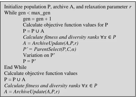
Figure 2.1: Algorithm Pseudo code, mechanisms unique to DREMA shown in italics
Besides the archiving relaxation parameter, r, mentioned previously, two internally defined relaxation parameters, rank relaxation parameter α and rank replacement parameter C,are used in the parent selection operator. These parameters are described more fully in Section
2.4.2.
2.4.1 Ranking Procedure
DREMA works by ranking a solution based on one objective fitness metric (its hypervolume
contribution in the OS) and the three DS distribution rankings described in Figure 2.3 (called
“dispersion,” “remoteness,” and “alternate” rankings). DREMA allows a solution with a
higher diversity rank to replace one of its nearest DS neighbors in the parent set, within an
allowable tradeoff in objective rank. DREMA retains optimal and near-optimal solutions in Initialize population P, archive A, and relaxation parameter r
While gen < max_gen gen = gen + 1
Calculate objective function values for P
P = P A
Calculate fitness and diversity ranks A = ArchiveUpdate(A,P,r)
P’ = ParentSelect(P,C,α)
Variation on P’ P = P’
End While
Calculate objective function values
P = P A
two different archives. The following sections describe the mechanisms by which DREMA
differs from the generic EA: fitness and diversity ranking, as well as procedures for parent
selection and archive updating.
2.4.1.1 Objective Space Ranking
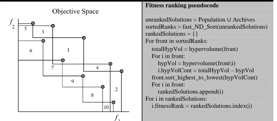
DREMA ranks objective fitness by using non-dominated sorting, as described in Deb et al.’s
NSGA-II [27], to successively find the non-dominated front of solutions in a set. Then the
solutions are ranked within each front by determining OS hypervolume contribution, as first
shown in SMS-EMOA [38] and used again in an EMO problem application by Dorn [16].
Within each successive front found by non-dominated sorting, solutions are ranked according
to the volume of hyperspace they dominate within that front. In Figure 2.2, for example,
each solution has a number representing its objective fitness rank. The solution ranked
number one dominates the largest hyperbox in its front. The second-ranked solution has the
second largest dominated hyperbox, and so on. Ranking continues in the second front with
the sixth ranked solution, which dominates the most hyperspace of any solution in its front.
Fitness ranking pseudocode
unrankedSolutions = Population Archives
sortedRanks = fast_ND_Sort(unrankedSolutions) rankedSolutions = {}
For front in sortedRanks:
totalHypVol = hypervolume(front) For i in front:
hypVol = hypervolume(front\i) i.hypVolCont = totalHypVol – hypVol front.sort_highest_to_lowest(hypVolCont) For i in front:
rankedSolutions.append(i) For i in rankedSolutions:
i.fitnessRank = rankedSolutions.index(i)
2.4.1.2 Decision Space Ranking
Three different metrics are used to rank solutions based upon decision space (DS) criteria. In
each case, the lowest (best) rank is given to the solution with the greatest distance or sum of
distances to certain neighboring solutions, as determined by three different mechanisms
described in Figure 2.3. The first mechanism, called “dispersion” ranking, sums the
distances to a solution’s two nearest neighbors in the DS. The dispersion ranking accounts
for the two nearest solutions to reduce the likelihood that two otherwise remote solutions will
eliminate each other based only on their proximity to each other. The second, “remoteness” mechanism, is based upon a solution’s distance to the nearest non-dominated solution in the
DS. This ranking system favors solutions located in areas of the DS that are unpopulated by
non-dominated solutions. Finally, the “alternate” ranking mechanism gives the highest rank
to the solution with the greatest DS distance to its nearest neighbor in the OS, for which it
can act as a more different, but similarly-performing alternative.
The calculations for the four rankings are completed in one loop of the population for each
solution, so each ranking measure does not constitute a significant marginal increase in
computation time. Once all solutions are ranked according to the one OS and three DS
measures, the archive is updated (see Section 2.4.3) and parents are selected with the
(a)
(b)
(c)
Dispersion ranking pseudocode:
for each solution, a, in Population: nearest = neighbor1
secondNearest = neighbor2 for each solution, b, in Population: if a != b:
if Distance(a,b) < Distance(a, nearest): secondNearest = nearest
nearest = b
a.dispersion = (Distance(a,nearest)) + Distance(a,secondNearest))
SortHighestToLowest(Population,dispersion) for each solution, a, in Population:
a.dispersionRanking = Population.index(a)
Remoteness ranking pseudocode:
for each solution, a, in Population: nearest = neighbor
for each solution, b, in ParetoFront: if Distance(a,b) < Distance(a,nearest): nearest = b
a.remoteness = Distance(a,nearest)
SortHighestToLowest(Population,remoteness) for each solution, a, in Population:
a.remotenessRanking = Population.index(a)
Alternate ranking pseudocode:
for each solution, b, in Population: nearestOS = neighbor
for each solution, c, in Population:
if OSDistance(b,c) < OSDistance(b,nearestOS): nearestOS = c
b.alternate = DSDistance(b,nearestOS) SortHighestToLowest(Population,alternate) for each solution, b, in Population:
b.alternateRanking = Population.index(b)
Figure 2.3: DREMA Decision Space (DS) diversity ranking mechanisms
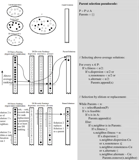
2.4.2 Parent Selection
During each generation, the current population and all archived solutions are searched for
feasible solutions whose objective rank and at least one of the diversity metrics are superior
to that of the average solution. These solutions are automatically added to the parent set.
The remaining n solutions are given n equal chances to be added to the parent set, until the parent set has been filled. This can be done either automatically (if it is an archived solution)
or by replacement (if one of its nearest DS neighbors is in the parent set). A solution can
replace its neighbor in the parent set if it is feasible, its objective rank is better or within α places of its neighbor’s rank and one of its diversity ranks is Cα places better than its
neighbor’s corresponding diversity rank. Figure 2.4 illustrates the parent selection and
replacement operator.
By allowing replacement of nearest DS neighbors by alternates with high dispersion,
remoteness, or alternate rankings, solutions are allowed to compete with other solutions on
the basis of their single area of greatest performance. The reason for enhancing each type of
diversity separately is to preserve the ability of the algorithm to provide useful alternatives,
whether they are identified by their similarity in objective performance to a particular
solution, by their maximal distance from another solution in the DS, or by their contribution
Parent selection pseudocode:
P = P A
Parents = {}
// Selecting above-average solutions:
For every x P: If x.fitness < n/2: If x.dispersion < n/2 or x.remoteness < n/2 or x.alternate < n/2: Parents.append(x)
// Selection by elitism or replacement:
While Parents < n: x = selectRandom(P) If x is feasible: If x is in A:
Parents.append(x) Else:
If x.neighbor is in Parents: If x.fitness ≤
x.neighbor.fitness + α: If x.dispersion ≤
x.neighbor.dispersion-Cα or x.remoteness
x.neighbor.remoteness-Cα or x.alternate ≤
x.neighbor.alternate – Cα: Parents.remove(x.neighbor) Parents.append(x)
Figure 2.4: DREMA parent selection and replacement operator
Above average rankings
Solution 2 is within rank relaxation from 1
Solution 2 replaces Solution 1 as a parent Solution 2 is
one of Solution 1’s nearest neighbors
rank1 – rank2
2.4.3 Archives
DREMA maintains two archives: a Pareto Front and a Diversity Archive. The two archives
are updated at the end of each generation by the mechanism described in Figure 2.5. A
user-defined relaxation distance, r, is used to determine whether a near-Pareto optimal solution will be retained in the Diversity Archive. A solution is archived if its objective function
values are within r percent of all of the objective function values of at least one non-dominated solution (as measured from the same reference point that is used to calculate
hypervolume). The reference point and the relaxation parameter selected affect the size and
diversity of DREMA’s final solution set.
Relaxation distance from Pareto Front
Allowed relaxation distance is determined as a percentage, r (e.g. 2%), of the distance of a solution’s nearest Pareto front neighbor from a reference point.
ParetoFront = nondominatedSort(Population) dominated = Population – ParetoFront for each solution, x’, in dominated: for each solution, x, in ParetoFront: for each objective, f:
if OSDistance(x’,refPoint) ≥ (1 – s)OSDisstance(x,refPoint):
DivArchive = DivArchive x’
Break
2.5 Performance Testing and Results
2.5.1 Performance Comparisons
Algorithm performance will be measured using the metrics described in Section 2.3. In the
OS, performance will be indicated by hypervolume. In the DS, performance will be
measured with several different metrics: the Solow-Polasky diversity metric (Equations 2.3
thru 2.5) [35] [36], Shir’s DS “diameter” (Equations 2.6 and 2.7) [17], Average Minimum
DS distance (Equation 2.8), Minimum Minimum DS distance (Equation 2.9), and Average
Distance from the Nearest OS neighbor (Equation 2.10).
The six test problems are provided in Table 2.1. DREMA’s performance will be compared
with three other algorithms, when results are available. To compare DREMA against other
diversity-seeking algorithms, Shir et al.’s results for the Niching-Covariance Matrix
Adaptation (N-CMA) algorithm [17] and Ulrich et al.’s results for the Diversity Integrating
Multi-objective Optimizer (DIOP) [35] are provided. To provide a point of reference,
particularly on hypervolume performance, against algorithms not seeking diversity, results of
an implementation of Deb et al.’s NSGA-II [27] are provided.
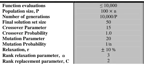
The algorithm settings provided in Table 2.2 were selected to provide meaningful
comparisons with the additional algorithm results reported in Tables 2.3 thru 2.8. The
number of function evaluations is kept at or below 10,000, which is the minimum for the
comparison algorithms considered. As some of the metrics calculated are affected by the
number of solutions, such as increased hypervolume caused by more dense non-dominated
fronts, greater SP diversity metrics caused by more distinct solutions, and the decreased
diversity in the distance-based metrics due to a more crowded DS, it is necessary to select
final solution sets from the archives maintained during the algorithm’s progression, that are
equal in size to those whose results are supplied for comparison. The methods for selecting
Table 2.1: Test Problems Characteristics and Settings
Problem Objectives
Variables Reference Point Diameter Objective Function Two-On-One [39] 2 2 (35,7) 8.4853 ( ) ( ) [ ] Omni Test [32] 2 5 (1,1)
13.4164 ( ) ∑ ( )
( ) ∑ ( ) [ ] Lame Superspheres [17] [40] 2 4 (2,2) 7.1040 ( ) ( )( ( )) ( ) ( )( ( ))
where ( ) ∑
[ ] [ ] EBN [38] 2 10 (2,2)
3.1623 ( ) (∑ | |
) ( ) (∑ | | ) [ ] Lame Scaled [17] [40] 3 7 (2,2,2) 2.6457 ( ) ( )( ( )) ( ) ( ) ( )( ( )) ( ) ( ) ( )( ( ))
where ( ) ∑
[ ] [ ] DTLZ2 [41] 3 7 (2,2,2) 2.6457 ( ) ( ( ))( ( ⁄ ) ( ⁄ )) ( ) ( ( ))( ( ⁄ ) ( ⁄ )) ( ) ( ( ))( ( ⁄ ))
where ( ) ∑ ( )
Table 2.2: DREMA settings Function evaluations Population size, P Number of generations Final solution set size Crossover Parameter Crossover Probability Mutation Parameter Mutation Probability Relaxation, r
Rank relaxation parameter, α Rank replacement parameter, C
≤ 10,000
100 n
10,000/P 50 15 1.0 20 1/n 10 %
3 2
2.5.2 Selection of Final Solution Sets
In addition to the two archives DREMA retains throughout the algorithm run, two additional
final set selection methodologies are used to trim the final number of provided solutions to
50. As some of the metrics are set size-dependent, this trimming is meant to achieve a valid
comparison with the final solution sets of size 50 obtained by the other algorithms. Best
Hypervolume Trimming (BH) selects 50 Pareto optimal solutions by eliminating excess
solutions with the smallest contribution to hypervolume. Diversity Grid Trimming (DG)
divides the range of each objective by the target set size (adjusted for possible duplication),
divided by the number of objectives. Then, for each objective increment, a solution is
selected with the highest OS or DS rank. In the case of duplicate selections, the set is then
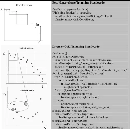
Best Hypervolume Trimming Pseudocode
finalSet = copy(totalArchives) While finalSet.size() > targetSize:
minContributor = argmin(finalSet, hypVolCont) finalSet.remove(minContributor)
Diversity Grid Trimming Pseudocode
finalSet = {}
for n in numberObjectives:
maxFitness[n] = max_fitnes_value(totalArchive) minFitness[n] = min_fitness_value(totalArchive) range[n] = maxFitness[n] – minFitness[n]
increment[n] = (range[n]/(targetSize*1.5/numberObjectives)) for i in (1,targetSize*1.5/numberObjectives):
for n in (1,numberObjectives): for x in totalArchives:
if maxFitness[n] ≥ x.fitness[n] ≥ minFitness[n]: neighbors[n].append(x)
for n in (1,numberObjectives): if length(neighbors[n]) == 1: finalSet.append(single_solution) else:
neighbors.sort(min(ranks))
finalSet.append(solution_with_best_rank) if finalSet.size() < targetSize:
while finalSet.size() < targetSize:
finalSet.append(totalArchives.min(ranks)) if finalSet.size() > targetSize:
while finalSet.size() > targetSize:
finalSet.remove(worst_ranked_ in_each_ neighborhood)
2.5.3 Results
The Distributed Evolutionary Algorithms in Python (DEAP) package, available online [42],
was used for the EMO framework, and most algorithm components not specific to DREMA.
Exceptions include hypervolume calculations, executed in C code available at
http://www.wfg.csse.uwa.edu.au/, implementing the algorithm developed by While et al.
[43]. A Python wrapper for this code was downloaded from http://www.swig.org/ [44].
DREMA results are reported for each test problem in Tables 2.3 thru 2.9, corresponding to
each metric. Algorithm performance is compared to the N-CMA [17], DIOP [35], and
NSGA-II [27] algorithms, when metric data are available from each study. Table 2.9
presents the clusters found in the Omni-Test problem, which has 243 global optima. The
number of clusters found by DREMA, DIOP, and the Omni Optimizer (as reported in [35])
are compared. For the three new diversity metrics defined in Section 2.3 (AM, MM, and
ADNO), the only data available are from the Python implementations of DREMA and
NSGA-II conducted for this study. In every table, the best average and standard deviation
for each problem are shown in bold. For the SP metric in Table 2.4 and the Omni Test
clusters found in Table 2.9, the top performer is only determined among the sets of size 50.
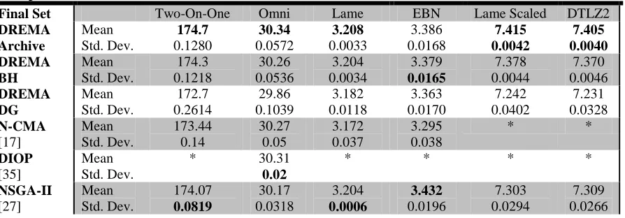
Table 2.3: Hypervolume Results; Results shown for 30 trials; Best average and standard deviation for each problem shown in bold
Final Set Two-On-One Omni Lame EBN Lame Scaled DTLZ2
DREMA Archive Mean Std. Dev. 174.7 0.1280 30.34 0.0572 3.208 0.0033 3.386 0.0168 7.415 0.0042 7.405 0.0040 DREMA BH Mean Std. Dev. 174.3 0.1218 30.26 0.0536 3.204 0.0034 3.379 0.0165 7.378 0.0044 7.370 0.0046 DREMA DG Mean Std. Dev. 172.7 0.2614 29.86 0.1039 3.182 0.0118 3.363 0.0170 7.242 0.0402 7.231 0.0328 N-CMA [17] Mean Std. Dev. 173.44 0.14 30.27 0.05 3.172 0.037 3.295 0.038 * * DIOP [35] Mean Std. Dev.
* 30.31
Table 2.4: Solow-Polasky Diversity Results; Results shown for 30 trials; Best average and standard deviation amongst the 50-solution sets for each problem shown in bold
Final Set Two-On-One Omni Lame EBN Lame Scaled DTLZ2
DREMA Archive Mean Std. Dev. 50.35 1.429 264.0 10.13 276.8 7.399 281.1 5.894 382.1 9.810 104.4 3.819 DREMA BH Mean Std. Dev. 11.78 0.2917 43.16 1.947 47.31 0.9462 48.00 0.6478 48.49 0.4237 25.51 1.061 DREMA DG Mean Std. Dev. 27.51 1.309 47.95 1.005 48.97 0.7028 48.86 0.5069 48.91 0.5232 36.58 1.516 N-CMA [17] Mean Std. Dev. * * * * * * DIOP [35] Mean Std. Dev.
* 48.7
0.90 * * * * NSGA-II [27] Mean Std. Dev. 14.48 0.5673 22.32 4.175 26.51 4.862 44.31 1.234 33.26 4.660 22.06 0.9422
Table 2.5: Shir Diversity Results; Results shown for 30 trials; Best average and standard deviation for each problem shown in bold
Final Set Two-On-One Omni Lame EBN Lame Scaled DTLZ2
DREMA Archive Mean Std. Dev. 0.1684 0.0107 0.3849 0.0110 0.4120 0.0065 0.5433 0.0083 0.3590 0.0056 0.2318 0.0043 DREMA BH Mean Std. Dev. 0.0735 0.0019 0.3697 0.0174 0.3919 0.0161 0.5440 0.0094 0.3558 0.0094 0.2293 0.0052 DREMA DG Mean Std. Dev. 0.1779 0.0122 0.3950 0.0115 0.4231 0.0120 0.5557 0.0073 0.3864 0.0092 0.2625 0.0080 N-CMA [17] Mean Std. Dev. 0.296 0.012 0.247 0.061 0.412 0.022 0.484 0.007 * * DIOP [35] Mean Std. Dev.
* 0.66
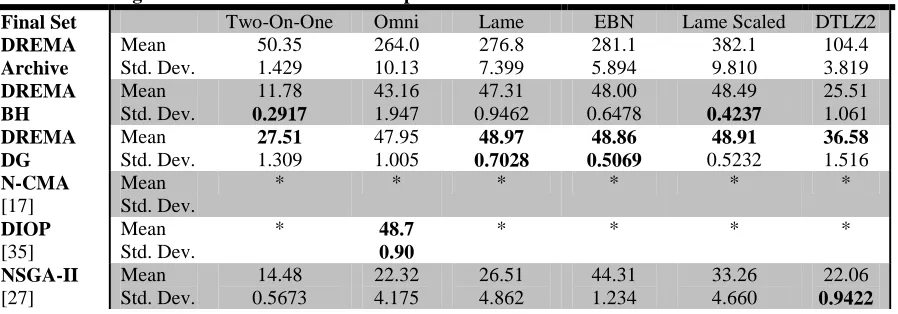
Table 2.6: Average Minimum (AM) Distance Results; Results shown for 30 trials; Best average and standard deviation for each problem shown in bold
Final Set Two-On-One Omni Lame EBN Lame Scaled DTLZ2
DREMA Archive Mean Std. Dev. 0.0342 0.0017 0.3863 0.0591 0.1842 0.0086 0.4730 0.0167 0.1884 0.0090 0.1146 0.0043 DREMA BH Mean Std. Dev. 0.0477 0.0021 1.313 0.1950 0.5844 0.0538 0.7379 0.0374 0.4929 0.0219 0.1639 0.0118 DREMA DG Mean Std. Dev. 0.1315 0.0101 1.825 0.1792 0.7408 0.0476 0.8292 0.0278 0.5489 0.0292 0.2638 0.0141 N-CMA [17] Mean Std. Dev. * * * * * * DIOP [35] Mean Std. Dev. * * * * * * NSGA-II [27] Mean Std. Dev. 0.0555 0.0050 0.1743 0.1114 0.1383 0.0437 0.6284 0.0519 0.2023 0.0363 0.1293 0.0118
Table 2.7: Minimum Minimum (MM) Distance Results; Results shown for 30 trials; Best average and standard deviation for each problem shown in bold
Final Set Two-On-One Omni Lame EBN Lame Scaled DTLZ2
Table 2.8: Average Distance to Nearest Objective (ADNO) Results; Results shown for 30 trials; Best average and standard deviation for each problem shown in bold
Final Set Two-On-One Omni Lame EBN Lame Scaled DTLZ2
DREMA Archive Mean Std. Dev. 0.4716 0.0627 4.059 0.1692 2.319 0.1047 1.297 0.0358 0.6858 0.0293 0.2019 0.0093 DREMA BH Mean Std. Dev. 0.0506 0.0030 3.808 0.3562 2.734 0.1652 1.203 0.0630 0.9168 0.0489 0.2015 0.0202 DREMA DG Mean Std. Dev. 1.207 0.2001 5.021 0.3389 3.018 0.2376 1.314 0.0480 1.032 0.0507 0.3555 0.0231 N-CMA [17] Mean Std. Dev. * * * * * * DIOP [35] Mean Std. Dev. * * * * * * NSGA-II [27] Mean Std. Dev. 0.0796 0.0160 1.384 0.6318 0.8072 0.4714 1.102 0.0753 0.3977 0.1309 0.1772 0.0178
Table 2.9: Clusters Found in Omni-Test; Results shown for 30 trials; Best average and standard deviation for each problem shown in bold
Final Set Clusters Found
DREMA Archive Mean Std. Dev. 147.5 15.05 DREMA BH Mean Std. Dev. 38.13 2.778 DREMA DG Mean Std. Dev. 39.83 2.531 DIOP [35] Mean Std. Dev. 39.9 3.7 Omni-Opt [32][35] Mean Std. Dev. 23.8 1.4
The full archive retained by DREMA found the best hypervolume of any algorithm in five
out of the six test problems, as shown in Table 2.3. This is to be expected, since the size of
the final solution set was large; however, even after final selection procedures reduced the set
size to 50 for proper comparison, DREMA’s BH and DG sets still were competitive with, or
outperformed, the other algorithms, including NSGA-II, which had only fitness pressure.
While NSGA-II sometimes achieves a smaller standard deviation of hypervolumes across the
three of the test problems. High hypervolume values with low standard deviations indicate
DREMA’s reliable OS convergence, even while seeking more diversity in the DS.
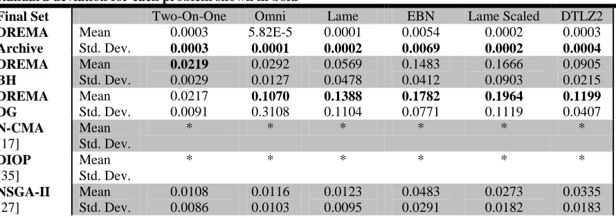
SP diversity metrics in Table 2.4 were not available for all of the algorithms. However,
DREMA achieved very nearly the highest possible value of 50 in a 50-solution set on four of
the problems, greatly exceeding NSGA-II, which serves as an example of a non-diversity
seeking algorithm. Exceptions include the Two-On-One and DTLZ2 problems, where only
DREMA’s DG set considerably surpassed NSGA-II’s SP diversity values, and the one
problem where another diversity-seeking algorithm’s performance is available: the Omni
Test problem, where DREMA’s BH and DG final solution sets are slightly outperformed by DIOP’s high SP diversity value. On four of the problems, DREMA’s BH or DG sets’ SP
values are the most robust, and on the remaining two problems, are competitive with most
robust performers (NSGAII on DTLZ2 and DIOP on Omni).
Table 2.5 shows that DREMA’s SD metrics are the top performers or competitive with the
top performers on four of the six problems (Lame, EBN, and Lame Scaled, and DTLZ2).
DREMA outperforms N-CMA and NSGA-II on the Omni Test problem, but cannot compete
with DIOP’s high SD diversity score, though DREMA’s SD values are highly robust, one of
its solution sets being the most robust of all the algorithms on five of the six problems. On
the Two-On-One problem, DREMA’s BH and DG sets are below N-CMA’s levels. This
could be attributable to the lower distinctiveness of the final solutions, as illustrated by
DREMA’s SP diversity values for that problem.
On the AM metric in Table 2.6, DREMA’s top performing solution set outperforms
NSGA-II’s by anywhere from 30 to 950 percent, with both the BH and DG sets outperforming
NSGA-II on five of the six problems. Because this metric is sensitive to the number of
solutions in the DS, comparing these sets to NSGA-II’s final set of the same size is most
meaningful; however, even DREMA’s larger full archive is competitive with NSGA-II’s AM
anywhere from 2 to 11 times, as shown in Table 2.7. Unfortunately, no data from the other
diversity-seeking algorithms are available for these metrics.
Table 2.8 shows DREMA’s ANDO measures for every solution set exceeding NSGA-II’s by
varying degrees (7 to 1816 percent) on all but one problem: Two-On-One. DREMA also has
higher precision within the 30 trials in every solution set on all but two of the problems
(Two-On-One and DTLZ2), and has the most robust solution set in every problem. The one
case where NSGA-II outperforms one of DREMA’s solution sets is the Two-On-One
problem, where the BH set has a slightly lower value than NSGA-II’s final set. With explicit
dependence on a similar measure during ranking and selection, it is no surprise that DREMA
performs consistently well on DS distance-based metrics, such as SD, AM, MM, and ADNO.
Of the 243 clusters in the Omni Test problem, Table 2.9 shows that DREMA’s BH and DG
sets (of normalized size) outperform the Omni-Optimizer in the number of global optima
found. The maximum number of clusters that could be represented in each solution set is
limited by the number of distinct solutions in the set (50). DREMA’s BH and DG sets have a
large number of their solutions falling in different clusters (an average of 38.13 and 39.83
across all trials). Although DREMA’s BH and DG sets are barely outperformed by DIOP’s
average of 39.9 clusters found, they have less variation than DIOP in the number of global
optima represented in each trial.
2.6 Observations
DREMA’s convergence to strong approximations of the Pareto front in 10,000 or fewer function evaluations is reflected in its final solution sets’ steadily high hypervolume values,
rivaling even NSGA-II, whose sole selection pressure is on objective fitness. In many cases,
gains in hypervolume tapered to near-optimal before the final generations. In fact, there is
reason to believe that DREMA’s diversity pressure also helps convergence in the OS, as side experiments showed DREMA’s hypervolumes exceeding those of a non-diversity version of
Judging from DREMA’s performance in the distance-based diversity metrics, it can be said
that the algorithm is effective in producing and retaining solutions that are diverse in the
specific ways sought by the ranking and selection systems. This is also supported by side
experiments which changed the emphasis placed on each ranking system during parent and
final selection, which subsequently increased or decreased the corresponding metrics closest
in definition to the objective, dispersion, diversity, or alternate ranking changed. This is an
intuitive result, and it shows DREMA’s promise in being adapted by users to more explicitly
foster the development of alternatives with the specific types of diversity that decision
makers seek.
When data were available, DREMA was often not the highest-performing diversity-seeking
algorithm on some of the diversity metrics. Although being outperformed by DIOP, and
occasionally N-CMA in SP and SD metrics, DREMA still showed competitive diversity
values, often much exceeding NSGA-II’s. This represents success in pursuing diversity,
while not at the expense of objective pressure. DREMA achieves highly competitive
hypervolume values, with consistently high robustness, demonstrating its usefulness as a
general purpose EA with the ability to generate high quality solutions for different test
CHAPTER 3 – SATISFYING MULTIPLE OBJECTIVES IN WASTEWATER NETWORK TREATMENT DESIGN
3.1 Introduction
Infrastructure management and planning in the water and wastewater sectors have seen a
shift during the last three decades. Traditional large-scale, supply-side investments in water
and wastewater services are now considered in competition with smaller-scale, non-structural
alternatives and technologies to meet new demand or increase service efficiency. As the
most readily exploitable water resources had already been developed and water resource
development began to shift to local governments, the economic, social, and environmental
costs of water use and expansion began to be realized by local stakeholders [12]. This shift
has increased the complexity of water resources planning, but it is also accompanied by
greater opportunity for strategy and innovation in decision-making practices. There has been
significant growth in optimization modeling and decision-making methods for water and
wastewater planning and management problems in the last three decades [13]. Despite the
advances made in these areas, no optimization model can address all decision criteria, and no
solution method has overcome all of the barriers to the adoption of optimization models as
common practice in water systems.
Barriers to effective solutions to water system optimization problems include incomplete
knowledge of systems, oversimplification or inaccuracies in defining objective functions, and
the fact that minimum cost solutions do not allow for uncertainties or for unmodeled factors
such as growth in demand or excess capacity that would be desirable in responding to
network failures [3]. Some of the technical barriers to water system optimization can be
overcome by ensuring sufficient diversity in the final solution set that enables presenting
decision makers with alternatives capable of better-satisfying modeled, unmodeled, tangible,
and intangible priorities. This chapter presents a diversity-preserving genetic algorithm
which draws from the rapidly growing foundation of evolutionary multi-objective algorithms
in water resources planning [13] [20], and the ongoing investigation of evolutionary
Modeling to Generate Alternatives (MGA) has been demonstrated using mathematical
models to solve the problem addressed in this chapter (e.g., [7] [14] [46]). As the mixed
integer linear programming (MILP) MGA-based approach used in this study establishes an
upper limit to the achievable difference of an alternative solution from its nearest
non-dominated neighbor, a meta-heuristic approach such as evolutionary algorithms (EAs) cannot
be expected to outperform the MGA/MILP approach in finding maximally different solutions
to any set of modeled objectives defined before the decision-making process, as shown by Loughlin et al. [9]. The analyses performed in this paper, however, aim to provide additional
insight into the performance of a diversity-preserving GA on a real-world wastewater
management problem, as compared to an MGA/MILP approach, under different diversity
measures and preference scenarios which could arise during the decision-making process.
The following section introduces the DuPage County, Illinois, regional wastewater example
problem, which has previously been modeled as a one-objective problem solved as a
mixed-integer linear program [7] [14] and later solved using a genetic algorithm and analyzed with
respect to an unmodeled second objective by Zechman and Ranjithan [11]. Also in Section
3.2, a second objective is defined and explained, to create a two-objective problem. In
Section 3.3, two solution methods are described: an MILP approach, and a problem-specific
solution repair operator to the new diversity preserving EA approach, Diversity Ranking
Evolutionary Multi-objective Algorithm (DREMA), described in Chapter 2. Section 3.4
compares the performance of DREMA to that of the MILP approach on the modeled
two-objective problem. Section 3.5 considers another decision priority that is not considered in
the model, and provides a comparison of the performance of DREMA and MILP solutions
with respect to an unmodeled, intangible objective. Section 3.6 supposes that another
quantifiable objective arises during the decision-making process, and provides post-analysis
comparisons of the DREMA and MILP solutions (for the dual-objective problem) with
respect to the third, unmodeled objective. Finally, the results are discussed in Section 3.7,
3.2 An Illustrative Regional Wastewater Treatment Problem
3.2.1 DuPage County Problem Formulation
A case study on the regionalization of wastewater treatment in DuPage County, Illinois, was
first presented by Nakamura and Brill in 1977 [14]. The case study area, as shown in Figure
3.1, includes 15 sites generating wastewater, of which 12 are potential treatment plant
locations, as well as 16 possible interceptor routes between sites. The mathematical
formulation of the problem has 28 binary variables indicating the construction of each
network component (ie., a treatment facility or interceptor), and 28 continuous variables
representing flow serviced by each component. Each potential treatment plant and
interceptor route has a fixed cost and a cost per unit of flow serviced (in cubic feet per
second). Constraints include maximum capacities for both treatment plants and interceptors,
as well as flow balance constraints at each site. A mathematical programming representation
of the problem (based on prior work by Nakamura and Brill [14]) is given in Equations 3.1
thru 3.5.
Minimize ∑ ∑ ∑ ∑ ∑ ∑ (3.1)
Such that ∑ ∑ (3.2)
(3.3)
(3.4)
{ } (3.5)
where FCj is the fixed cost for treatment plant j; GCij is the fixed cost for interceptor from source i to j; PCj is the unit cost of treatment at plant j; ICij is the unit cost of transport through interceptor from i to j; Yj is the binary variable indicating whether treatment plant j is
active; Zijis the binary variable indicating whether interceptor from i to j is active; PQjis the amount of water treated at plant j; IQij is the amount of water transported through interceptor
from i to j; Lj is the amount of wastewater generated at source j; Mj is the maximum treatment capacity at plant j; Nij is the maximum flow capacity through interceptor from i to j. All flow variables are in cubic feet per second (cfs).
3.2.2 Second Objective Formulation
The effective generation of alternative solutions to this problem would allow the necessary
flexibility to consider the economic, social, and environmental implications of regional
wastewater management decisions. For instance, wastewater treatment plants and
interceptors certainly experience economies of scale in their construction and operation.
Although the least-cost solution may promote a centralized design, other factors such as the
historical bias towards decentralization, or the required flexibility in localized treatment or
expansion of wastewater facilities, may cause decision makers to gravitate towards other
options. Certain environmentally sensitive areas may draw protection against construction or
development, necessitating a revision in network design plans. Out of a desire to reduce the
impact of development or to retain water resources closer to their source, communities may
considering system resilience, in that a larger treatment plant may be less vulnerable to minor
hazards but more catastrophic in the event of a large service disruption [47].
The degree of centralization, therefore, may very well be a decision priority at the outset of
the design. If decision makers wish to prioritize decentralization, then the second objective
modeled as the summation of internodal flow could be minimized, as shown in Equation 3.6.
The smaller the quantity of wastewater transported between sources, the more decentralized
the network. Decentralization also presents a direct correlation both to pumping energy used
in the case of a forced-flow network, and to the dislocation of discharges from wastewater
sources, which can be undesirable from the standpoint of low-impact development advocates,
as well as to source communities with the potential for water shortages. Figure 3.2a shows
the minimum cost solution, as found in previous studies [7] [11] [14]. Figure 3.2b is one of
the possible minimum flow solutions (trivially found by constructing all possible wastewater
treatment plants and transporting only the flow from each site without a potential WWTP).
(a) (b)
3.3 Solution Methods
3.3.1 A Mixed-Integer Linear Programming (MILP) Approach
After adding the second objective function (Equation 3.6), the non-dominated Pareto front
was found using an MILP approach. An ε-constraint approach was used to optimize one
objective function, while constraining the other objective value to a value of ε [48].
Minimize ( ) (3.7)
Subject to:
( ) (3.8)
Equations 3.2 – 3.5
To approximate the entire non-dominated front to the desired degree of precision, δ,
successively generated constraints were used to optimize internodal flow while incrementally
increasing the cost constraint by δ (USD 1000). After the Pareto front was found, the
following method was used to generate alternative designs for each Pareto optimal solution.
3.3.1.1 An MILP Modeling to Generate Alternatives (MGA) Approach
The following method is one of several possible ways to use MGA to find a diverse set of
alternative solutions within the specified relaxation from the two-objective Pareto Front
solutions [1]. Assuming a problem such as the two-objective minimization defined in
Equations 3.1 to 3.6, this MGA approach finds a desired number, n, of maximally different alternatives (X1,… Xn), for each non-dominated solution, X0. Maximum difference, D, is defined here as the number of binary variables for which an alternative solution, Xn, differs from a non-dominated solution, X0. First, X1 is found by maximizing the difference function,
D, from X0, subject to the constraints in Equations 3.2 to 3.5.
Maximize ∑ | | ∑ ∑ | | (3.9)
Subject to:
( ) ( ) for f = (1,2) (3.10)
Equations 3.2 – 3.5
where Xn (for n > 0) is the alternative solution currently being generated, and s is a defined relaxation target from the optimal function values. To find the second set of alternatives, X2, Equation 3.9 is reformulated into Equation 3.11, to find a solution X2, that maximizes the sum of the differences D from X0 and X1, still subject to the same constraints.
Maximize ∑ | | | | ∑ ∑ | | | | (3.11)
A variety of Modeling to Generate Alternatives (MGA) approaches have already been used