Developing a Mathematical Model to Predict Power Consumption in Turning of EN-24 and EN-31 under Dry and Wet Conditions

Developing a Mathematical Model to Predict

Power Consumption in Turning of EN-24 and

EN-31 under Dry and Wet Conditions

Darshan M. Katgeri

, Anand V. Kulkarni

, Sachin C. Kulkarni

1

Lecturer, Department of Mechanical Engineering, Jain College of Engineering, Belgaum, Karnataka, India

2

Assistant Professor, Department of Mechanical Engineering, KLSGIT, Belgaum, Karnataka, India

3

Assistant Professor, Department of Mechanical Engineering, KLSGIT, Belgaum, Karnataka, India

ABSTRACT: The objective of this study is to develop a better understanding of the effects of spindle speed (S), cutting feed rate (f) and depth of cut (d) on power consumption and to build a suitable mathematical model. Such an understanding can provide insight into the problems of estimating the power requirements of machined surfaces when the process parameters are adjusted to obtain a certain responses like power consumption. This paper aims at presenting the techniques that can be employed to predict the effect of speed, feed and depth-of-cut to generate information that will allow us to understand and model the relationship between the process variables and measures of the process performance

KEYWORDS: Orthogonal Array (OA), Taguchi, Regression, Power Consumption

I. INTRODUCTION

Machining is one of the most important activities in manufacturing. It is of great importance not only to the machine tool industries but also to the entire class of engineering manufacturing industries using machine tools in one form or the other. Although extensive research has been done in this field the metal cutting industries using various machine tools continue to suffer from a major drawback of not utilizing the machine tools at their full potential; in order to address this problem various parameters that affect this problem have to be analysed. One way of doing this is to carefully design an experiment that will allow us to measure the process parameters using experience and knowledge. Design of Experiments is a tool to develop an experimentation strategy that maximizes learning using a minimum of resources. Most of the standard experimental designs can be generated once the experimental objective, the number (and nature) of the design variables, the nature of the responses and the economical number of experimental runs have been defined. Generating such a design will provide the user with the list of all experiments to be performed in order to gather the required information to meet the objectives. With designed experiments there is a better possibility of testing the significance of the effects and the relevance of the whole model. The concept of using OA’s to design an experiment was first introduced by Taguchi.

The general machining problem can be described as the achievement of a predefined product quality with given equipment, cost and time constraints. This paper aims at presenting the techniques that can be employed to predict the effect of speed, feed and depth-of-cut to generate information that will allow us to understand and model the relationship between the process variables and measures of the process performance. Well-chosen experimental designs maximize the amount of information that can be obtained for a given amount of experimental effort and might lead to a more rapid solution.

interaction effect and perform Taguchi’s S/N analysis. The effect of used petrol engine oil (SAE-40) on power consumption of EN-24 and EN-31 is studied.

The predicted model mainly depends on critical parameters like spindle speed, feed rate, depth of cut and their interaction among each other. This allows for the determination of optimal machining strategies and tooling for the required machining processes. The resulting benefits will allow for the machining process to become more productive and competitive.

Bhattacharya et al [1] investigated the effects of cutting parameters on power consumption by employing Taguchi techniques. Their results showed a significant effect of cutting speed on the power consumption, while the other parameters did not substantially affect the responses. The literature survey reveals that traditional experimental design procedures are too complicated and not easy to use. A large number of experimental works have to be carried out when the number of the process parameters increases. To solve this problem, the Taguchi method uses a special design of orthogonal arrays to study the entire parameter space with only a small number of experiments [2]. Lin [3] has formulated the experimental results of surface roughness and cutting forces by regression analysis, and modeled the effects of them in his study using S5SC steel. Sood et al [4] studied the specific energy where the power of machining is one of the parameter affecting the specific energy. Faleh et al [5] have reported that the power consumption is one of the most important parameters for online monitoring of tool conditions. It is can be seen that power consumption is increased with increase in cutting speed, feed rate and depth of cut. This is quite obvious because as all this three parameters increases, the material removal rate also increase which forcing the system to spend more power.

Based on the experiment and the analysis it is observed that used petrol engine oil (SAE 40) reduces the power requirement during machining.

Paper is organized as follows. Section II describes the Methodology. Section III describes the experimentation and selection of factors, levels and OA’s. Section IV focuses on the power consumption. Section V deals elaborately with the results obtained and the mathematical equations used to predict the power consumption. The main effects plot and the interaction plot are shown in this section. Finally, Section VII presents conclusion.

II. RELATEDWORKANDMETHODOLOGY

The literature survey reveals that there is lot of scope for research and exploration in the area of power consumption. Hence power consumption is selected as the output parameter. A thorough study on machining and of Taguchi methodology was done and then the input and output parameters were selected. An L9 orthogonal array was selected though the resolution of this orthogonal array is low. The predicted values are in close match with actual values of power consumption and the results are within 90% confidence level.

The steps mentioned below are followed as guidelines to design and conduct the experiment.

1. Define the process objective.

2. Determine the design parameters affecting the process. Parameters are variables within the process that affect the performance measure such as speed, feed, depth of cut etc. that can be easily controlled.

3. Create orthogonal arrays for the parameter design indicating the number of columns and conditions for each experiment. The selection of orthogonal arrays is based on the number of parameters and the levels of variation for each parameter.

4. Conduct the experiments indicated in the completed array to collect data on the effect on the performance measure.

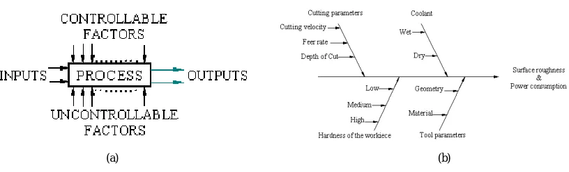
(a) (b)

Fig .1. (a) General model of process or system (b) Factors affecting Power Consumption

III.EXPERIMENTATION AND SELECTION OF FACTORS, LEVELS AND ORTHOGONAL ARRAY

In this study, work pieces of steel EN-24 and EN-31 of dimensions 20 X 70 mm are used. The machining was carried out on a Kirloskar lathe using single point carbide tool. The experiments were conducted for both dry and lubricated (wet) conditions; used petrol engine oil (SAE-40) was utilised as lubricant, sufficient oil was smeared all-round the work piece using a brush. The factors chosen for the experiments are speed (S), feed (f), and depth of cut (d). Level 1 represents low level, Level 2 is the intermediate level and Level 3 is high level; for Level 1 speed, feed and depth of cut are 630(m/min), 0.08(mm/rev) and 0.5(mm) respectively. The values for Level 2 & Level 3 are given in Table 1.

Table. 1. Table shows factors and levels used in the experiment.

S.No Cutting parameter (Factor) Level 1 Level 2 Level 3

1 RPM/Cutting velocity, rpm/(m/min) 630/40 840/50 1000/60

2 Feed rate(mm/rev) 0.08 0.11 0.16

3 Depth of Cut (mm) 0.5 1.0 1.5

To select an appropriate orthogonal array for experiments, the total degrees of freedom need to be computed. The degrees of freedom are defined as the number of comparisons between process parameters that need to be made to determine which is better and specifically how much better it is. A three level process parameter counts for two degrees of freedom. The degrees of freedom associated with interaction between two process parameters are given by the product of the degrees of freedom for two process parameters. In this study an L9 orthogonal array is used. Each cutting parameter is assigned to a column. The design matrix was generated using Minitab V14. Table 2 represents the coded values of the factors. The values 1, 2 and 3 represents low level, intermediate level and high level. These values correspond to the values given in Table 1.

Table. 2. Table shows design matrix used in the experiment.

S.No 1 2 3 4 5 6 7 8 9

Speed 1 1 1 2 2 2 3 3 3

Feed 1 2 3 1 2 3 1 2 3

Depth of Cut 1 2 3 2 3 1 3 1 2

IV.MACHININGPERFORMANCEMEASURES

V. EXPERIMENTALRESULTS

The experiments have been performed on EN-24 and EN-31 materials in accordance with the design matrix obtained earlier.The main effects and the Interaction plot have been plotted using Minitab V14. The graphical comparison of power consumption for both the materials under dry and lubricated condition is done using MS Excel.Table 3shows the tangential force F(tan), feed force F(feed), and radial force F(rad), resultant of the forces, experimental value power consumption and the predicted value of power consumption for EN-24 under non lubricated conditions.The experimental values are obtained by using the equations given below.

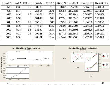
Table. 3. Values of power consumption for EN-24-dry

Speed, S Feed, f DOC, d F(tan) N F(feed) N F(rad) N Resultant Power(prdt) Power(Calc)

630 0.08 0.5 78.480 9.81 68.67 104.7421 0.065981 0.069828

630 0.11 1 255.06 78.48 176.58 319.9925 0.219591 0.213328

630 0.16 1.5 431.64 127.53 304.11 543.1941 0.363983 0.362129

840 0.08 1 284.49 98.1 107.91 319.6916 0.223952 0.213128

840 0.11 1.5 353.16 98.1 353.16 508.9868 0.324596 0.339325

840 0.16 0.5 176.58 19.62 255.06 310.8393 0.204928 0.207226

1000 0.08 1.5 382.59 78.48 421.83 574.8693 0.386128 0.383246

1000 0.11 0.5 196.21 78.48 117.72 241.8916 0.156676 0.161261

1000 0.16 1 206.01 39.24 235.44 315.2965 0.217040 0.210198

1000 840 630 0.35 0.30 0.25 0.20 0.15 0.16 0.11 0.08 1.5 1.0 0.5 0.35 0.30 0.25 0.20 0.15 Speed M e a n o f P o w e r R e s u lt a n t Feed DOC

Main Effects Plot for Power resultant(dry) Data Means

0.16 0.11

0.08 0.5 1.0 1.5

0.35 0.25 0.15 0.35 0.25 0.15 Speed F eed DO C 630 840 1000 Speed 0.08 0.11 0.16 Feed

Interaction Plot for Power resultant(dry) Data Means

(a) (b) Fig 1. (a)Main Effects plot for Power Resultant for EN-24-Dry (b) Interaction for Power Resultant for EN-24-Dry

Fig 1. (a) shows that the power consumption increases between speed range 630 to 840 and remains constant thereafter; it increases gradually with feed and DOC. Fig 1 (b) shows the interaction plot of Speed v/s Feed, Speed v/s DOC, and Feed v/s DOC. At medium and high speeds and high feed rate the power consumption is almost same. The lowest power consumption is observed at low speed and low feed as expected. It is recommended to use medium DOC to get optimum power consumption. Lowest power consumption is obtained at low speed and low DOC and highest power consumption is obtained at high speed and high DOC as expected. The power consumption is observed to increase with increase in feed and DOC, at medium DOC the power consumption is same for all feeds. It is recommended to use medium DOC to get optimum power consumption.

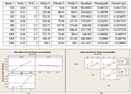
Table. 4 gives the forces, resultant and the values of power consumption obtained in turning EN-24 under lubricated (wet) condition. The resultant is the square root of the sum of squares of all the forces.

Table .4. Values of power consumption for EN-24-wet

Speed, S Feed, f DOC, d F(tan) N F(feed) N F(rad) N Resultant Power(prdt) Power(Calc)

630 0.08 0.5 78.48 9.81 58.86 98.58928 0.065726 0.0611734

630 0.11 1 235.44 68.67 68.67 254.6824 0.169788 0.1691513

630 0.16 1.5 353.16 98.1 294.3 470.0618 0.313375 0.3234978

840 0.08 1 235.44 78.48 127.53 279.0251 0.232521 0.2827232

840 0.11 1.5 323.73 107.91 274.68 438.058 0.365048 0.3379104

840 0.16 0.5 176.58 49.05 206.01 275.7291 0.229774 0.2357524

1000 0.08 1.5 372.78 78.48 392.4 546.902 0.546902 0.549374

1000 0.11 0.5 186.39 29.43 215.82 286.6804 0.28668 0.269744

1000 0.16 1 196.2 29.43 98.1 221.3237 0.221324 0.238864

1000 840 630 0.40 0.35 0.30 0.25 0.20 0.16 0.11 0.08 1.5 1.0 0.5 0.40 0.35 0.30 0.25 0.20 Speed M e a n o f P o w e r R e s u lt a n t Feed DOC

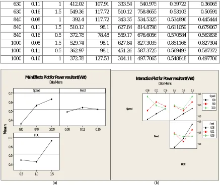
Main Effects Plot for Power resultant(Wet) Data Means

0.16 0.11

0.08 0.5 1.0 1.5

0.4 0.2 0.0 0.4 0.2 0.0 Speed Feed DO C 630 840 1000 Speed 0.08 0.11 0.16 Feed

Interaction Plot for Power resultant(Wet) Data Means

(a) (b)

Fig 2. (a) Main Effects plot for Power Resultant for EN-24-Wet (b) Interaction for Power Resultant for EN-24-Wet

Fig 2. (a) shows that the power consumption increases as speed increases; it gradually decreases as feed rate increases. There is no much change in power consumption from DOC 0.5 to 1.0 mm but then after it increases drastically. Fig 2 (b) that the unit variation of power consumption for all speeds and low feed rate is much pronounced and it is observed to decrease at medium feed rate, the unit variation is lowest at highest feed rate. At medium and high speeds and high feed rate the power consumption is almost same. The lowest power consumption is observed at low speed and low feed as expected. The power consumption is observed to increase with increase in speed and DOC, at medium DOC the power consumption is almost same for speeds 840 and 1000.At medium DOC the power consumption is same for all feeds. It is recommended to use medium DOC to get optimum power consumption. Lowest power consumption is obtained at low feed and low DOC and highest power consumption is obtained at low feed and high DOC.

Predicted regression model for power consumption is

Power (prdt) wet= -1.3635 + 0.001761S+ 13.755f-0.2683d -0.015839Sf +0.000517Sd -0.486fd +0.003864

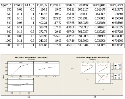
Table. 5. Experimental values of power consumptionfor EN-31-dry

Speed, S Feed, f DOC, d F(tan) N F(feed) N F(rad) N Resultant Power(prdt) Power(Calc)

630 0.08 0.5 196.2 49.05 304.11 365.2167 0.243478 0.243478

630 0.11 1 441.45 196.2 353.16 598.41 0.39894 0.39894

630 0.16 1.5 588.6 245.25 539.55 835.2914 0.556861 0.556861

840 0.08 1 402.21 117.72 637.65 763.0389 0.635866 0.635866

840 0.11 1.5 529.74 137.34 470.88 721.952 0.601627 0.601627

840 0.16 0.5 372.78 29.43 667.08 764.7397 0.637283 0.637283

1000 0.08 1.5 519.93 225.63 402.21 694.9885 0.694988 0.694988

1000 0.11 0.5 343.35 49.05 647.46 734.5063 0.734506 0.734506

1000 0.16 1 421.83 137.34 461.07 639.8346 0.639835 0.639835

1000 840 630 0.7

0.6

0.5

0.4

0.16 0.11 0.08

1.5 1.0 0.5 0.7

0.6

0.5

0.4

Speed

M

e

a

n

Feed

DOC

Main Effects Plot for Power resultant(dry) Data Means

0.16 0.11

0.08 0.5 1.0 1.5

0.6

0.4 0.2 0.6 0.4

0.2

Speed

Fee d

DOC

630 840 1000 Speed

0.08 0.11 0.16 F eed

Interaction Plot for Power resultant(dry) Data Means

(a) (b)

Fig 3. (a) Main Effects plot for Power Resultant for EN-31-Dry (b) Interaction for Power Resultant for EN-31-Dry

Fig 3. (a) shows that the power consumption increases gradually as the levels of all the factors increase. Fig 3 (b) shows interaction plots for Speed v/s Feed, Speed v/s DOC, and Feed v/s DOC for EN-31-dry. At low speed the power consumption increases with increase in feed. At medium speed the power consumption remains fairly same. At high speed the power consumption increases slightly with increase in feed from 0.08 to 0.11 and then decreases for feed range 0.11 to 0.16. At low speed the power consumption increases with increase in DOC. At medium speed the power consumption remains fairly same. At medium and low feed rate and medium DOC the power consumption is almost same. It is recommended to use mentioned feeds and DOC’s to get optimum power consumption.

Predicted regression model for power consumption is

Power (prdt) dry= -1.6981 + 0.001369S +7.716f +1.1053d -0.006394Sf -0.000953Sd -2.463fd + 0.004577

Table. 6 gives various values of forces and power consumption obtained during experimentation of EN-31 under lubricated (wet) conditions. The best value obtained at speed, feed, depth of cut of 1000, 0.08 and 1.5 respectively.

Table. 6. Experimental values of Power Consumption for EN-31-wet

Speed, S Feed, f DOC, d F(tan) N F(feed) N F(rad) N Resultant Power(prdt) Power(Calc)

630 0.11 1 412.02 107.91 333.54 540.975 0.39722 0.36065

630 0.16 1.5 549.36 117.72 510.12 758.8655 0.53103 0.50591

840 0.08 1 392.4 117.72 343.35 534.5325 0.534896 0.445444

840 0.11 1.5 510.12 98.1 627.84 814.8798 0.611059 0.679067

840 0.16 0.5 372.78 78.48 559.17 676.6056 0.570584 0.563838

1000 0.08 1.5 529.74 98.1 627.84 827.3035 0.851168 0.827304

1000 0.11 0.5 362.97 98.1 451.26 587.3725 0.569493 0.587372

1000 0.16 1 372.78 127.53 304.11 497.7065 0.548848 0.497706

1000 840 630 0.7

0.6

0.5

0.4

0.16 0.11 0.08

1.5 1.0 0.5 0.7

0.6

0.5

0.4

Speed

M

e

a

n

Feed

DOC

Main Effects Plot for Power resultant(Wet) Data Means

0.16 0.11

0.08 0.5 1.0 1.5

0.9

0.6

0.3

0.9

0.6

0.3 Speed

Feed

DOC

630 840 1000 Speed

0.08 0.11 0.16 Feed Interaction Plot for Power resultant(Wet)

Data Means

(a) (b)

Fig 4. (a) Main Effects plot for Power Resultant for EN-31-Wet(b) Interaction for Power Resultant for EN-31-Wet

Fig 4. (a) shows that the power consumption increases gradually with increase in speed. For feed rate it is fairly constant; it decreases slightly from DOC 0.5 to 1.0 and increases drastically from DOC 1.0 to 1.5 mm. Fig 4 (b) shows interaction plots for Speed v/s Feed, Speed v/s DOC, and Feed v/s DOC for EN-31-wet.At low speed the power consumption increases with increase in feed. At all speeds and high feed rates the power consumption remains fairly same. At high speed the power consumption decreases slightly with increase in feed from 0.08 to 0.11 and then decreases further for feed range 0.11 to 0.16.At low speed the power consumption increases with increase in DOC. At low and medium speed the power consumption graph shows same trend, the power consumption decreases slightly with increase in DOC and thereafter increases with increase in DOC. The unit variation in power consumption is observed to be uniform at all feeds and low and hence it is recommended to use medium DOC’s with various feed rates. Better Ra value is obtained at low speed and low DOC.

Predicted regression model for power consumption is

VI.COMPARISONOFPOWERCONSUMPTIONFOREN-24ANDEN-31

(a) (b)

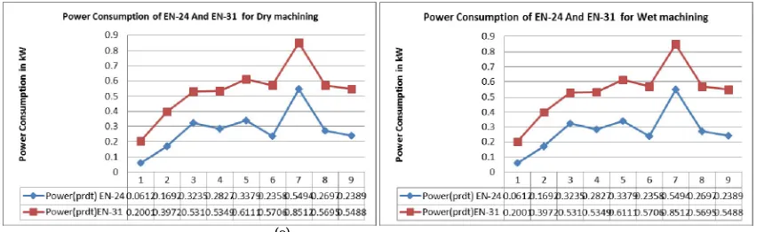
Fig 5. (a) Power Consumption of EN-24 and EN-31 for Dry machining (b) Power Consumption of EN-24and EN-31 for wet machining

Fig 5. (a) & (b) show that the results obtained are in 90% confidence level i.e. the predicted and the experimental values are close to each other. The nature of the graphs obtained by platting the results is shown in Fig 5 (a) and (b). The graphs are plotted in Microsoft Excel. The equations mentioned above can be used to predict the power consumption with good accuracy with the range. This has been confirmed by conducting conformation and validation experiments. The results may or may not yield the correct results beyond the range.

VII. CONCLUSION

The predicted values and measured values are fairly close which indicates that the developed power consumption prediction models can be effectively used to predict the power consumption from the cutting process with 90% confident intervals for both case (dry and wet). Discarded engine oil of petrol car can be used as a lubricant to reduce the power consumption as it is observed that the surface roughness of materials under consideration also improves. However, its chemical effects on the material have to be studied.

REFERENCES

1. Bhattacharya, S. Das, P. Majumder, A. Batish, Estimating the effect of cutting parameters on surface finish and power consumption during high speed machining of AISI 1045 steel using Taguchi design and ANOVA, Prod. Eng. Res. Dev. Volume 3, pages 31–40, 2009

2. E. Bagci, S. Aykut, A study of Taguchi optimization method for identifying optimum surface roughness in CNC face milling of cobalt-based alloy (stellite 6), Int. J. Adv. Manuf. Technol. Volume 29, Issue 9, pages 940–947, 2006

3. Lin W. S., Lee B. Y. Modeling the surface roughness and cutting forces during turning. Journal of Materials Processing Technology, Volume 108, pages 286-93,2001.

4. Sood R., C. Guo and S. Malkin, Turning of hardened steels. Journal of Manufacturing Processes, Volume 2, Issue 3, pages 187-193, 2000. 5. Faleh A. Al-Sulaiman, M. A. Basser, A. K. Sheakh. Use of electrical power for online monitoring of tool condition. Journal of Materials