Invalidation Analysis and Revision of Polar Format Algorithm for Dechirped Echo Signals in ISAR Imaging

(1)

Invalidation Analysis and Revision of Polar Format Algorithm

for Dechirped Echo Signals in ISAR Imaging

Yang Liu*, Na Li, Bin Yuan, and Zengping Chen

Abstract—In this paper, we present a detailed analysis on the invalidation of the polar format algorithm (PFA) for the dechirped echo signals in inverse synthetic aperture radar (ISAR) imaging. After the data-driven translational motion compensation, the polar section of the dechirped signals is often undermined, and then the PFA is invalid. A revision method by range shifting is proposed to compensate the echo signals, and the standard polar section is obtained. An improved performance was achieved on the simulated and real data experiments. The theoretical analysis and the proposed method are conﬁrmed.

1. INTRODUCTION

Inverse synthetic aperture radar (ISAR) can generate 2D images for a non-cooperative moving target in military and civilian applications. The high range resolution is proportional to the bandwidth of the transmitted signal. The high cross-range resolution is achieved using a synthetic antenna aperture generated by the rotational motion of the target [1]. The range resolutionρ_r is deﬁned asρ_r=c/(2B), where c is the light velocity, B is the signal bandwidth. The cross-range resolution ρ_a is deﬁned as ρa =λ/(2Θ), where λis the signal wavelength, and Θ is the target rotation angle within the coherent processing interval (CPI).

Generally, in a traditional ISAR imaging system, a linear frequency modulation (LFM) signal is transmitted, and the echo signals are then dechirped to decrease the receiver bandwidth. Several popular ISAR signal processing algorithms are proposed in the literatures, such as the Range-Doppler algorithm (RDA) [2], the Keystone algorithm [3, 4] and the polar format algorithm (PFA) [5–7]. The RDA is applicable when the rotation angle is small to ensure there is no significant migration through range cells (MTRC) and time-varying Doppler in the echoed signal. The Keystone algorithm is effective for the migration through range resolution cells (MTRRC) caused by the target rotation with constant velocity. However, it is invalid for the migration through cross-range resolution cells (MTCRRC). The PFA was first used to compensate the MTRC in SAR imaging [5]. It was introduced in ISAR imaging later. The PFA algorithm firstly interpolates the observed signal from polar sector support region to the Cartesian rectangular region. The fast Fourier transform (FFT) is followed to focus the ISAR image [8, 9]. Since both the range and the Doppler curve are permitted in the PFA, the maximum rotation angle is significantly wider for the PFA algorithm compared to the Keystone and the RDA.

In practical applications, the PFA requires accurate estimation of the rotation parameter to interpolate the complex data points. However, once the translational motion is compensated, the polar section of the dechirped signals is often undermined, since the rotation center (RC) is deviated from the reference range. In that case, the PFA is invalid. This paper ﬁrst analyzes the PFA algorithm and the factors causing the invalidation detailedly. Then we propose a method to revise the polar sector of the echoes. The PFA algorithm is applied to the revised signal in order to obtain a focused imaged. Experimental results were carried on both of the simulated and real data to demonstrate the accuracy of the analysis and the eﬀectiveness of the improved method.

Received 17 June 2014, Accepted 1 September 2014, Scheduled 3 September 2014

* Corresponding author: Yang Liu ([email protected]).

(2)

The rest of the paper is organized as follows. The dechirped echo signals and polar format algorithm are introduced in Section 2. Section 3 analyzes the invalidation of the PFA algorithm in ISAR imaging for dechirped signal and presents an improved PFA. Experimental results and analysis are reported in Section 4, followed by conclusions in Section 5.

2. DECHIRPED ECHO SIGNALS AND PFA ALGORITHM 2.1. Dechirped Signal Model Formulation

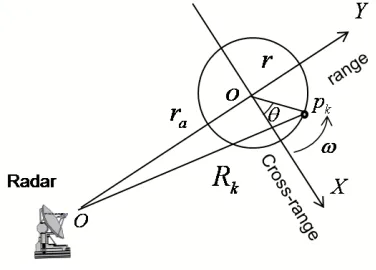
The point scatterer model is commonly used in radar imaging systems [9]. If the translational motion has been fully removed, the geometry of radar imaging is depicted in Fig. 1. The instantaneous distance from the scattering pointp_kwith position (x_k, y_k) to the radar can be approximated as:

Rk(t)ra(t) +xksinθ(t) +ykcosθ(t) (1) where r_a is the range from target RC to the radar, and θ(t) is the instantaneous rotation angel at arbitrary time.

Figure 1. Geometry of the scattering pointp.

In an ISAR imaging system, a LFM signal is often transmitted, and then the echo is dechirped to reduce the receiver bandwidth. Supposing that the target consists ofK point scatterers, the return signals can be expressed as:

sRˆt, tm = K

k=1

σkrecttˆ−(2Rk(tm)/c)/Tp

exp −j2π

fcˆt−(2R_k(t_m)/c)+1 2γ

ˆ

t−(2R_k(t_m)/c)2

(2)

whereσ_k,candf_care the backward scattering coeﬃcient, light speed and carrier frequency, respectively. γ denotes the chirp rate of the transmitted signal. Since the target motion is much lower than the speed of light, the full time t= ˆt+tm is expressed in the form of fast time ˆt and slow timetm=mTp, where mare integers andTp denotes the pulse width. Suppose that the reference point (RP) isoand its range to radar isr0(t). Then after the dechirping, the received signal is given as:

sR2

ˆ

t, tm = K

k=1

σkrectˆt−(2 (R_k(t_m)−r0(t_m))/c)/T_p

exp j4π c

fc+γˆt−2R0(tm)/cRps k(tm)

exp (jψ_k(t_m)) (3)

where

Rps k(tm) =Rk(tm)−r0(tm), ψ(tm) = 4_cπγ2 R 2

(3)

Rps k(t_m) is the instantaneous range from P_k to o, and ψ(t_m) is the residual video phase (RVP). Generally, the RVP can be removed easily, when dealing with small targets.

Let us denote f =γˆt−2r0(t_m)/c and substitute it into (3), and then one can obtain:

sR3(f, tm) = K

k=1

σkrect (f/γ)−(2 (Rk(_Ttm)−r0(tm))/c) p

exp j4π

c (fc+f)Rps k(tm)

(5)

Assume that the RP locates at the RC, i.e.,r0(t) =ra(t), then one can obtain Rps k from (1): Rps kxksinθ(t) +ykcosθ(t) (6) SinceR_k(t_m)r0(t_m) for small targets, the dechirped echo signals can be ﬁnally expressed as:

sR4(f, θ) = K

k=1

σkrect _Bf

exp j4π

c (fc+f) (xksinθ(t) +ykcosθ(t))

(7)

whereB =γT_p denotes the signal bandwidth.

2.2. Polar Format Algorithm for Dechirped Signals

Since both the range and Doppler curve are permitted in the PFA, the maximum rotation angles for the PFA algorithm are wider. Let K_R=−(4π/c)(f_c+f), then the phase term of (7) can be expressed as:

Φ(θ) =K_R(x_ksinθ+y_kcosθ) =K_xx_k+K_yy_k (8) where (θ, K_R) is the polar format of (K_x, K_y) in a Cartesian coordinate system. If the target rotation angle Θ is known, the target image can be reconstructed from 2D Fourier Transform (2D-FT). However, the FT algorithm requires a rectangular raster distribution of the data points, and the signal model can acquire a sector support region. Therefore, interpolation of the observed signal on a polar sector support region to a Cartesian rectangular system is required. As it is shown in Fig. 2, the radial wavenumber KR satisﬁes:

KR∈[KR1, KR2] = 4π

c

fc− B

2, fc+ B

2

(9)

The azimuth wavenumber is (4π/λ)·Θ.

An illustration of the PFA algorithm is shown in Fig. 3. If K_R2cos Θ ≤ KR1, the interpolation error will increase with Θ increasing, which results in a large vacant space in the wavenumber spectrum ﬁlled with stripe in the Fig. 3. Then, the maximum rotation angle for PFA is:

Θ_{P F A}= 2 cos−1 KR1 KR2

= 2 cos−1 1−0.5μ

1 + 0.5μ (10)

Figure 2. Wavenumber spectrum of echo signals after de-chirping.

(4)

(a) (b) (c) (d)

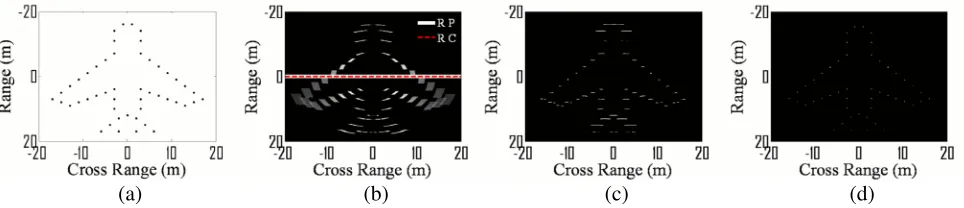
Figure 4. Imaging results of a simulated aircraft with the rotation center being the same as the reference point. (a) Scatterers model. (b) RD image. (c) Image after Keystone transform. (d) Image after PFA.

where μ=B/f_c. According to (10), Θ_{P F A} is merely a function of independent of the target size and the range resolution. Therefore, Θ_{P F A} is much larger than Θ_RD and Θ_Keystone. The ISAR images for a simulated aircraft are presented in Fig. 4. The aircraft is composed of 49 point caterers with equal reﬂectivity. The size of the aircraft shown in Fig. 4(a) is 20 m×20 m. The radar transmits LFM signals with a carried frequency of 15 GHz and a bandwidth of 2 GHz. The range resolutionρr= 0.075. In order to obtain high cross-range resolution matched with the range resolution, the target coherent rotation angel is set to Θ = 0.1 rad and the rotational velocity is set toω= 0.05 rad/s. The RC and RP are both located at (0 m,0 m) in the target coordinate system. The time of coherent processing interval is T_{CP I} = 2 s, the pulse number is M = 1024, and the pulse repetition frequency (PRF) is 1000 Hz. Meanwhile, the number of range bins in high resolution range proﬁle (HRRP) is N = 1024.

Figure 4(b) shows the ISAR image achieved by the RDA algorithm without any compensation. The blurring eﬀects caused by the MTRC can be found in both of the range cell and Doppler cell. The obtained ISAR image using the Keystone algorithm is shown in Fig. 4(c). It can be seen that the blurring in range cells caused by MTRRC is compensated, but the blur in Doppler cells still remains. Fig. 4(d) presents the ISAR image obtained by the PFA algorithm, where the target scatterers are optimally focused.

3. ANALYSIS OF PFA AND THE IMPROVED METHOD 3.1. Analysis and Simulation of the Invalidation of the PFA

According to (6) and (7), when the RC is located at the cell of the RP, the phase term of the dechirped signals can be expressed in polar format. Thus we can use the standard PFA algorithm to obtain a focused ISAR image without MTRC, as it is shown in Fig. 4. However, in practical applications, the RC is not always the same as the RP. Assume that the distance ofr0(t) andr_a(t) is Δr =r_a(t)−r0(t), (6) and (7) can be expressed as follows:

R_{ps k} Δr+x_ksinθ(t) +y_kcosθ(t) (11)

s

R4(f, θ) = K

k=1

σkrect f B

exp j4π

c (fc+f) (Δr+xksinθ(t) +ykcosθ(t))

(12)

Then, the phase term of (7) can be expressed as:

Φ(θ) =K_R(Δr+x_ksinθ+y_kcosθ) =K_RΔr+K_xx_k+K_yy_k (13)

whereKR=−(4π/c)(fc +f).

(5)

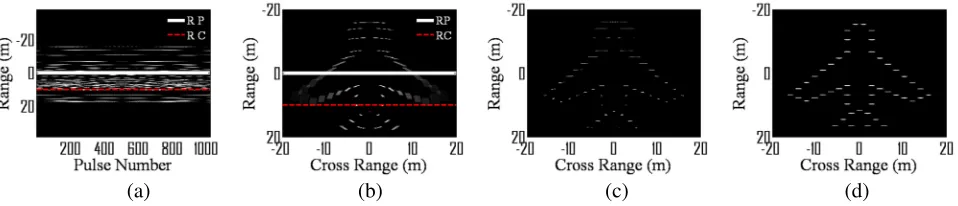
(a) (b) (c) (d)

Figure 5. Analysis of the PFA algorithm. (a) HRRPs of the simulated aircraft. (b) Image by RDA. (c) Image after Keystone transform. (d) Image by traditional PFA.

(0 m,0 m). The ISAR image achieved by the RDA is shown in Fig. 5(b) and the imaging result achieved with the PFA algorithm is shown in Fig. 5(d). Compared to the image in Fig. 4(d), the blur in Fig. 5(b) was not fully overcome by PFA.

3.2. The Improved PFA Algorithm

According to the theoretical analysis of the PFA algorithm, if the RC on slant range is not overlapped with the RP, the MTCRRC in ISAR imaging cannot be compensated using the PFA algorithm. In order to resolve this problem, the dechirped signals after translational compensation are shifted in slant range, and the RC is located at the center of the HRRP. As a result, the shifted signals follow the standard polar format.

It is known that the RP is located at the center of the HRRP. Therefore, the location of RC in HRRP is r_a(t) = Δr = ra(t)−r0(t). When the estimation value Δ˜r of Δr is obtained, s_R₄(f, θ) is shifted in the slant range, and the new dechirped signalss_R5(f, θ) can be written as:

sR5(f, θ) = s_R₄(f, θ)·exp −j4π

c (fc+f) Δ˜r

= K

k=1

σkrect _Bf

exp j4π

c (fc+f) [(Δr−Δ˜r) + (xksinθ(t) +ykcosθ(t))]

(14)

If the value of Δ˜r is equal to Δr, then Δr−Δ˜r0. The shifted signals in (14) become:

sR5(f, θ) = s_R 4(f, θ)·exp −j 4π

c (fc+f) Δ˜r

= K

k=1

σkrect _Bf

exp j4π

c (fc+f) (xksinθ(t) +ykcosθ(t))

(15)

From formula (15), the shifted signals have the same format as (7). s_R₄(f, θ) is revised to standard polar format. When the PFA algorithm is performed on the revised signals sR5(f, θ), the MTRC of s

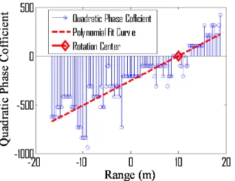
R4(f, θ) is compensated. Note that in Eq. (14), the RC should be estimated firstly. Many approaches have been proposed in the literatures for the RC estimation in ISAR imaging [10–14]. Here, we utilize the integrated cubic phase function (ICPF) to estimate rotation motion information. The ICPF extends the CPF and provides improved estimation performances of multi-component linear frequency modulated signals [11]. Fig. 6 shows the estimation coefficient of quadratic phase along the slant-range using ICPF. The RC is located at the range of 10.1 m, since the absolute value of the quadratic phase coefficient is minimized.

(6)

Figure 6. Coeﬃcient of quadratic phase estimated by ICPF method.

(a) (b)

Figure 7. The results of the revised PFA in Fig. 5. (a) HRRPs after range shift. (b) Image after revised PFA.

4. EXPERIMENT AND PERFORMANCE ANALYSIS

In the ﬁrst experiment, simulated data of aircraft (MIG-25) [1] were used. The aircraft is composed of 120 point scatterers with equal reﬂectivity. The radar transmits LFM signals with a carried frequency of 9 GHz and a bandwidth of 512 MHz. It was assumed that the aircraft had rotational motion only.

Figure 8(a) shows the image obtained by using RDA without any compensation, where the blurring eﬀects caused by the MTRC are signiﬁcant. The RC is located at −4.1 m, which is estimated by ICPF in Fig. 8(g) and highlighted by the dashed line in Fig. 8(c). Fig. 8(b) presents the ISAR image after MTRRC compensation, where the slant range migration has been corrected, and the cross range migration can still be found. As shown in Fig. 8(d), since the RC was not located at the same position as the RP, the image after PFA was still blurred. With the proposed ICPF estimation of RC, the HRRPS of shifted signals are shown in Fig. 8(e), and the image after PFA interpolating is shown in Fig. 8(f), where the MTRC was fully compensated.

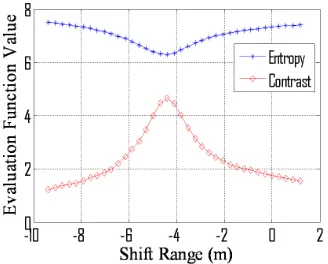
Figure 9 depicts the ISAR image entropy [15] and contrast [16] after PFA interpolating with diﬀerent shift range. The more focused the image is, the smaller the entropy is, and the larger the contrast is. The minimized entropy and the maximized contrast are achieved when the shift range is −4.1 m. It illustrates that more closed between the shift range and RC, more focused the compensated ISAR image is and consequently the more eﬃcient the PFA is.

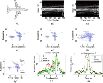
In the second experiment, the real data provided by ATR National Defense Science and Technology Key Laboratory were used. The data were collected by ground-based imaging radar. The target is a stably ﬂying airplane of Boeing 737, whose model is shown in Fig. 10(a). The carrier frequency is 10 GHz and the bandwidth is 1 GHz.

(7)

(a) (b) (c)

(d) (e) (f)

(g)

Figure 8. Simulated experiment of MIG-25. (a) RD image. (b) ISAR image after MTRRC. (c) Original HRRPs. (d) ISAR image after PFA. (e) HRRPs after range shift. (f) ISAR image of shifted signals after PFA. (g) Coeﬃcient of quadratic phase estimated by ICPF method.

Figure 9. The entropy and contrast of the image after PFA with diﬀerent shifted ranges.

(8)

(a) (b) (c)

(d) (e) (f)

(g) (h) (i)

Figure 10. Real data experiment of Boeing 737. (a) Model of Boeing 737. (b) Original HRRPs. (c) HRRPs after range shift. (d) Image after RDA. (e) Image after Keystone algorithm. (f) ISAR image after traditional PFA. (g) ISAR image after impoved PFA. (h) PSF of scatterer 1 along cross-range dimension. (i) PSF of scatterer 2 along cross-range dimension.

one utilizes PFA on the dechirped signals directly, the image is blurred in the cross-range direction. The HRRPS of shifted signals and the image after PFA interpolating are shown in Figs. 10(c) and(g), respectively. One can observe from Fig. 10(g) that more focused image was obtained by the proposed method. From Fig. 10(g), two dominant scatterers are chosen in range−19.6 m and−11.5 m. We plot the dominant scatterers corresponding to diﬀerent algorithms respectively along cross-range and range dimensions in Figs. 10(h) and (i) in order to show the improvement on the point spread function (PSF) by the use of the improve PFA. From Figs. 10(h) and (i), we note that the blur caused by MTRC both in range and cross-range dimensions was compensated by the proposed method.

Moreover, we use image entropy and contrast value to evaluate the focused images in Fig. 10, which are presented in Table 1. It is notable in Table 1 that a well focused ISAR image was obtained by using the improved PFA.

Table 1. Entropy and contrast evaluation.

RDA Keystone Traditional PFA Improved PFA

Entropy 9.23 8.92 12.3 8.37

(9)

5. CONCLUSION

The limitations of the traditional PFA algorithm for the dechirped echo signals in ISAR imaging is analyzed in this paper. The separation of RC and RP leads to the distributions of the 2-D scatterers mismatching the polar format. As a result, the image is blurred in the cross-range from PFA. In order to overcome the degradation, the RC in HIRRP is estimated by ICPF, and the dechirped signals after translational compensation are shifted in slant range accordingly. Consequently, the shifted signals follow the standard polar format. Experiments on simulated and real data show that the proposed method provides a promising performance improvement.

ACKNOWLEDGMENT

This work was supported by the National Natural Science Foundation of China (No. 61002025). The authors would like to thank Dr. Q. Q. Lin for providing the experimental data. The authors would also like to thank the editors and the anonymous reviewers for their helpful comments and suggestions.

REFERENCES

1. Chen, C. C. and H. C. Andrews, “Target motion induced radar imaging,” IEEE Trans. Aerosp. Electron. Syst., Vol. 16, No. 1, 2–14, 1980.

2. Zhou, F., X. Bai, M. Xing, and Z. Bao, “Analysis of wide-angle radar imaging,”IET Radar, Sonar and Navigation., Vol. 5, No. 4, 449–457, 2011.

3. Xing, M., R. Wu, J. Lan, and Z. Bao, “Migration through resolution cell compensation in ISAR imaging,”IEEE Geosci. Remote Sens. Lett., Vol. 1, No. 2, 141–144, Apr. 2004.

4. Wang, Y. and Y. C. Jiang, “A novel algorithm for estimating the rotation angle in ISAR imaging,” IEEE Geosci. Remote Sens. Lett., Vol. 5, No. 4, 608–609, Oct. 2008.

5. Carrara, W. G. and R. S. Goodman, Spotlight Synthetic Aperture Radar Signal Processing Algorithms, 157–189, Artech House, Boston, MA, 1995.

6. LeCaillec, J.-M., “SAR remote sensing analysis of the sea surface by polynomial ﬁltering,” IEEE Trans. Signal Process., Vol. 24, No. 4, 105–107, Jul. 2007.

7. Yu, T., M. D. Xing, and B. Zhen, “The polar format imaging algorithm based on double chirp-Z transforms,”IEEE Geosci. Remote Sens. Lett., Vol. 5, No. 4, 610–614, Oct. 2008.

8. Yang, Z. M., G. C. Sun, and M. D. Xing, “A new fast back-projection algorithm using polar format algorithm,”2013 Asia-Pacific Conference on Synthetic Aperture Radar, 373–376, 2013.

9. Mensa, D. L.,High Resolution Radar Imaging, 1224, Artech House, Dedham, MA, 1981.

10. Munoz-Ferreras, J. M. and F. P´erez-Mart´ınez, “Uniform rotational motion compensation for inverse synthetic aperture radar with non-cooperative targets,” IET Radar Sonar Navig., Vol. 2, No. 1, 25–34, Jan. 2008.

11. Zhang, W. C., Z. P. Chen, and B. Yuan, “Rotational motion compensation for wide-angle ISAR imaging based on integrated cubic phase function,” IET International Radar Conference 2013, Vol. 1, No. 5, 14–16. Apr. 2013.

12. Wang, M., A. K. Chan, and C. K. Chui, “Linear frequency-modulated signal detection using Radon-Ambiguity transform,”IEEE Trans. Signal Processing, Vol. 46, No. 3, 571–586, Mar. 1998. 13. O’Shea, P., “A new technique for estimating instantaneous frequency rate,”IEEE Signal Processing

Lett., Vol. 9, No. 8, 251–252, Aug. 2002.

14. Hu, J. M., W. Zhou, and Y. W. Fu, “Uniform rotational motion compensation for ISAR based on phase cancellation,” IEEE Geosci. Remote Sens. Lett., Vol. 8, No. 4, 636–641, Jul. 2011.

15. Wang, J., X. Liu, and Z. Zhou, “Minimum-entropy phase adjustment for ISAR,”IEE Proc. Radar Sonar Navig., Vol. 151, No. 4, 203–209, Aug. 2004.