Bistatic EM Scattering Analysis of an Object above a Rough Surface
Using a Hybrid Algorithm Accelerated with the Adaptive
Cross Approximation Method
Mohammad Kouali* and Noor Obead
Abstract—Calculating the RCS (Radar Cross Section) of two 3D scatterers needs to numerically solve a set of integral equations involving numerous unknowns. Such a 3D problem cannot be solved easily with a conventional Method of Moments (MoM) by using a direct LU inversion. Thus, hybridization between the Extended Propagation-Inside-Layer Expansion (E-PILE) and the Physical Optics approximation (PO) significantly reduces the memory requirements and CPU time. The resulting method called E-PILE+PO. In this work, we take advantage of the rank-deficient nature of the coupling matrices, corresponding to the interactions between scatterer 1 (the object) and scatterer 2 (the rough surface), to further reduce the complexity of the method by using the Adaptive Cross Approximation (ACA).
1. INTRODUCTION
In recent years, composite electromagnetic scattering from an object near a randomly rough surface has attracted considerable interest in the fields of radar surveillance, target identification, object tracking, etc.
Many methods have been proposed to solve scattering problem as a two-dimensional (2D) scattering problem [1–9]. Other methods deal with scattering problems as three-dimensional (3D) problem [10–17]. As expected, it is significant for practical applications to study the case of three dimensional problems. For large 3D problems, exact methods such as MoM are limited to the memory requirements. From that point, some methods proposed assumptions to simplify the calculations. For example, in [10] a hybrid method combines Kirchoff Approximation (KA) with MoM to study the scattering from 3D perfect electric conductor located above 2D dielectric rough surface. In [11], KA is used to derive a half-space Green function with the rough surface interface, and the MoM is applied in a complete 3D problem.
The works in [13, 14] propose assumptions to compute the coupling between the scatterers from the four-path model. In [15, 16], a proposed method called Finite-Difference Time Domain (FDTD) approach is used to discuss the scattering of a 3D object located above a 2D rough surface. An efficient numerical PILE (Propagation-Inside-Layer Expansion) method for computing the field scattered by rough layers is proposed in [4], then it is extended to solve a 3D problem called Extended-Propagation Inside Layer Expansion (E-PILE) [5].
For a large scenario, the work in [6] proposes a method that combines E-PILE with FBSA (Forward-Backward Spectral-Acceleration) method to calculate the local interaction on the rough surface and combined E-PILE with PO (Physical Optics) to compute the interaction on the object. Moreover, in [17] the forward-backward method is proposed to calculate the local interaction on the rough surface
Received 20 February 2019, Accepted 5 June 2019, Scheduled 17 June 2019
* Corresponding author: Mohammad Kouali (mkoali@staff.alquds.edu).
for a 3D problem. Furthermore, there have been other techniques to accelerate the computations like Complex Multipole Beam Approach (CMBA) as in [18], and this method uses a series of beams at the boundary instead of one beam. These beams are called Gabor functions, and this combination reduces the size of the matrix. CMBA is combined with MoM in [19]. The Impedance Matrix Localization method (IML) is introduced in [20]. This technique introduces new special basis functions and test functions that localize the significant interactions and use them, and as a result the required memory is reduced.
In [21], a proposed purely algebraic method called ACA is used to accelerate the electromagnetic computations of MoM. In [22], ACA method is combined with E-PILE and FBSA to solve a 2D problem with a huge number of unknowns.
Very recently, a bi-iteration model is proposed in [23], and the model is expressed by an outer and inner iteration. The proposed model effectively solves more complicated scattering problem from a 3D object located above a 2D rough surface.
In this paper, the ACA method is combined with the hybrid E-PILE+PO method to solve a 3D problem. To solve this problem, the E-PILE method is combined with the physical optics (PO) approximation to calculate the local interactions on both the object and the rough surface as in [25], then the ACA is applied to compress the coupling matrices to accelerate the coupling steps of E-PILE. As a result, the coupling matrices are strongly compressed without a loss of accuracy, and the memory requirement is then strongly reduced.
2. MATHEMATICAL FORMULATIONS
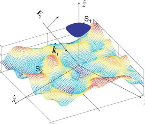
Let us consider an incident electromagnetic (EM) plane wave that illuminates the system composed of two perfect electric conductors (PEC) scatterers (object+rough surface) as shown in Fig. 1. The incident electromagnetic fields are written as
Ei(R) = ˆeieiki·R, H
i(R) = η1 0
ˆ
ki×Ei(R), (1)
where k is the wave number, ˆk a unit vector that gives the direction of the wave propagation, and η0 =
μ0\0 the intrinsic impedance of the air. Note that the time harmonic convention ejωt is assumed and suppressed throughout this paper. Solving the scattering problem is done by finding the electric surface current on the first scatterer (S1) and the second scatterer (S2).
To obtain the first coupling integral equation betweenS1 and S2, we use the boundary conditions on scatterer 1 (the object)S1,∀R ∈S1
ˆ
n1×Hi(R)+ ˆn1×−
S1
J1(R1)×∇R1G(R1,R)dS
local interactions
+ˆn1×
S2
J2(R2)×∇R2G(R2,R)dS
coupling interactions
= 1 2J1(R
), (2)
where−SdS is the principal value integral;G(R1,R) = exp(−ik0r)/4πris the free-space Green function withr the distance between the two pointsR1 and R; and J1,J2 are the electric currents on the two scatterers S1 and S2, respectively. G(R2,R) = exp(−ik0r)/4πr is the free-space Green function with r the distance between the two points R2 and R.
Using the boundary conditions on scatterer 2 (the rough surface)S2, the second coupling integral equation ∀R ∈S2 is obtained from
ˆ
n2×Hi(R)+ ˆn2×−
S2
J2(R2)×∇R2G(R2,R)dS
local interactions
+ˆn2×
S1
J1(R1)×∇R1G(R1,R)dS
coupling interactions
= 1 2J2(R
), (3)
Equations (2) and (3) can be explained as the total current on the surface. TakingS1as an example: the total current is the current from the incident wave, the surface current that occurs on the surface from local interactions, and the current that is produced as a result of the interaction occurring because of the presence of the second scatterer.
In order to solve the integral equations for two scatterers using MoM, we first discretize the two surfaces, and each surface is divided into small segments, then the surface current is calculated at each segment. The pulse function is used as the basis functions and delta functions as the test functions. The result of applying MoM is a linear system of the form ¯ZX =b, and this linear system describes the total scene. In detail, the unknown vectorX contains all the unknown surface currents for scatterer 1 and scatterer 2 in the form
X= X1
X2
(4)
where X1 is the surface current on the first scatterer, and X2 contains the surface currents for the second scatterer. X1,X2 are expanded in the form
X1= ⎡ ⎢ ⎢ ⎢ ⎢ ⎣
J1(R11) J1(R21)
.. .
J1(RN11) ⎤ ⎥ ⎥ ⎥ ⎥ ⎦ (5) and
X2= ⎡ ⎢ ⎢ ⎢ ⎣
J2(R12) J2(R22)
· · · J2(RN22)
⎤ ⎥ ⎥ ⎥
⎦ (6)
Here, N1, N2 are the numbers of unknowns in the first and second scatterer, respectively. As can be noticed, X vector has a dimension of (N1 +N2)×1. For a 3D problem, the current on each segment should represent the ˆx,yˆ,ˆz components of the current, so J1(R1) = Jx1xˆ+Jy1yˆ +Jz1zˆ and J2(R2) = Jx2ˆx+Jy2yˆ +Jz2ˆz. The column vector b which represents the incident field is equal to (b= ˆn×Hi), and it has a dimension of ((N1+N2)×1) and is described as
b= b1 b2
(7)
as a matrix of the sub-matrices in the form
¯ Z=
¯
Z1 Z¯12 ¯
Z21 Z¯2
(8)
Here ¯Z1 is the impedance matrix for the first scatterer from the local interaction on its surface as if it is alone in free space, in other words, the impedance matrix without any effects of the existence of the other scatterer. Moreover, ¯Z21 is the impedance matrix that describes the coupling between the two scatterers. In the same way, ¯Z2 is the impedance matrix of the second scatterer without any effects of the first scatterer, and ¯Z21 describes the effect of the coupling happens because of the existence of the first scatterer. To summarize, the linear system of the form ¯ZX=b is represented in the form:
¯
Z1 Z¯12 ¯
Z21 Z¯2
X1 X2
= b1 b2
(9)
The direct way to solve this system is to find ¯Z−1 and multiply it withb, thenX= ¯Z−1b. This solution is acceptable when the size of ¯Zis small, and this is limited to small (≤10λ) size of scatterers. A direct solution divides the impedance matrix into two parts called Lower and Upper (MoM-LU), then the calculations are done, and the MoM-LU will be the reference solution for our results since it is an exact solution for the system X= ¯Z−1b. The RCS from the proposed method will be tested and compared with RCS obtained from the MoM-LU.
As the size of the impedance matrix increases, the memory needed and the computational time for the inverse of ¯Z rise rapidly making it not an efficient way. Indeed, it calculates the inverse of the impedance matrix in an efficient way. E-PILE gives the surface current at the first scatterer as follows [17]
X1 =
Y10 = ¯Z−11(b1−Z¯21Z¯−21b2), p= 0 Y1(p)= ¯Mc,1Y(1p−1), p >0
(10)
where p is the order and refers to the number of interactions between the two scatterers, and ¯Mc,1 is the characteristic matrix and equals to:
¯
Mc,1= ¯Z−11Z¯21Z¯−21Z¯12, (11)
Similarly, the surface current at the second scatterer is expressed as
X2 =
Y20 = ¯Z−21(b2−Z¯12Z¯−11b1), p= 0 Y2(p)= ¯Mc,2Y(2p−1), p >0
(12)
where
¯
Mc,2= ¯Z−21Z¯12Z¯−11Z¯21, (13)
To reduce the calculations, E-PILE method is combined with PO approximation on both scatterers as in [24], and the surface current at the first scatterer (the object) is given by
Y0
1 = 2(b1−Z¯212b2), for p= 0 Y1(p)= ¯Mc,1Y(1p−1), for p >0
(14)
where ¯Mc,1 = 2 ¯Z212 ¯Z12.
Similarly, the surface current on the second scatterer (rough surface) is given by
Y20= 2(b2−Z¯122b1), for p= 0 Y2(p)= ¯Mc,2Y(2p−1), for p >0
(15)
where ¯Mc,2 = 2 ¯Z122 ¯Z21.
To summarize, after applying PO approximation at the two scatterers, the equations of the currents and the characteristic matrix are simplified significantly, and there is no need to calculate ¯Z−11and ¯Z−21. This reduces the time and memory used. In the following sections, PO1 indicates that the physical optics approximation is applied on scatterer 1, and PO2 indicates that PO is applied on scatterer 2.
3. E-PILE COMBINED WITH PO AND ACCELERATED BY ACA
In the previous section, PO approximation is combined with E-PILE to accelerate the computations of the local interactions on each scatterer (E-PILE+PO1+PO1). In this section, the ACA is used to accelerate the computations of the coupling between the two scatterers ( ¯Z21, ¯Z12) of complexity O(N1N2).
ACA is first introduced in [21], and it proposes an adaptive method to approximate matrix by multiplication of two approximated rectangular matrices. From that time, ACA was widely used for several reasons, one of them is its pure algebraic structure, that makes ACA easily used with other existing methods without any changes in the method structure. Moreover, using ACA, as will be discussed later, does not need full foreknowledge of the matrix. In other words, there is no need to compute all elements of the matrix. ACA chooses some elements to approximate the whole matrix, and these are the only elements to be calculated. To have a clear understanding about ACA, consider matrix
¯
Z with dimensions m×n. ACA approximates ¯Zm×n by a new matrix ˜Zm×n, and the approximated matrix is a multiplication of two rectangular matrices ¯V,U¯, in the form of [21]:
˜
Zm×n= ¯Um×rV¯r×n, (16)
where ¯U,V¯ are the rectangular matrices; r is the effective rank of the matrix ¯Zm×n;ui is the ith row of the matrix ¯U; and vi is the ith column of the matrix ¯V. From that equation, since the rank of the matrix is less than or equal to the minimum dimension of the matrix (r min(m, n)), the ACA takes its importance. Instead of save an impedance withm×nentities, ACA provides ((m+n)×r) elements to be saved, which is very efficient when we deal with matrices of large sizes. If we consider ¯R as the error matrix between the impedance matrix ( ¯Z) and approximated matrix ( ˜Z), then the ACA aims to achieve
R¯m×n=Z¯m×n−Z˜m×nεZ¯m×n (17)
where εis a given tolerance, and • denotes the matrix Frobenius norm, which is calculated by the square root of the sum of the absolute squares of the matrix elements. The choice of the εdepends on the application and the required accuracy of the results. After determining the value of ε, ACA starts to generate ¯Uand ¯V. The matrices ¯U and ¯V are constructed by selecting rows and columns from the
¯
Zmatrix, while ¯U and ¯V are generated, and the algorithm generates an approximate error matrix ˜R, which is equal toZ −¯ Z˜. Each time a new row or column of ¯Zis chosen, the corresponding error vector (row or column) is calculated by subtracting the actual column or row vector from the corresponding column or row vector of the approximate matrix that has been constructed in the previous iteration. The key point of choosing row or column returns to the index where the largest enter of the last computed error column or vector is located. At the end of ACA algorithm, the two matrices ¯U and ¯V are filled, and ACA is terminated when the following condition is satisfied
R¯εZ¯. (18)
Since the full knowledge of ¯Z is not necessary, ACA provides an estimation to the norm of ¯Z when computing the error matrix ¯R, and the norm of the error matrix is estimated after thekth iteration as
R(k)U
kVk, (19)
and
Z¯2
Z˜2=U¯(k)2V(k)2 =Z˜(k−1)2+ 2 k−1
j=1
uTj uk·vjvTk+uk2vk2, (20)
Recall that the equation to calculate the unknown currents on scatterer 1 by combining PO with E-PILE
is in the form
X01= 2(b1−Z¯212b2), for p= 0 X(1p)= ¯Mc,1Y(1p−1), for p >0
(21)
Similar equation to Eq. (21) can be written for scatterer 2. Once the equation ¯ZX=b is solved for X, the scattered fields are computed by using Huygens principle on the electric current densities, and the normalized Radar Cross Section (NRCS) of the two scatterers can be calculated by
NRCS = lim
R→∞4πR
2Es2
2ηPi , (22)
in which Es is the total scattered electric field in the far field region, andPi is the incident power.
4. NUMERICAL RESULTS
In this section, the ACA is applied to approximate the coupling matrices ¯Z12 and ¯Z21, then the calculations of X1,X2,M¯c,1 and ¯Mc,2 using this approximation will significantly accelerate the time needed and the memory used in the computations.
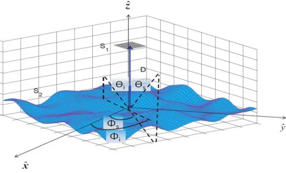
To implement the proposed method, consider that the scenario of a plate of dimension 1λ0×1λ0 is located above rough surface of dimension 8λ0×8λ0 which obeys a Gaussian process with a Gaussian height spectrum of root mean square height σz = 0.2λ0, and correlation lengths are Lcx =Lcy = 1λ0. The two scatterers are separated by distance of 5λ0, and sampling steps are Δx= Δy =λ0/10. The geometry of the problem is shown in Fig. 2. The number of unknowns: N1 = 300, N2 = 19,200.
Figure 2. Composite model of plate above a rough surface.
The surface height auto correlation function is a Gaussian type:
Cz(x, y) =σ2ze
− x2 L2cx−y
2 L2cy
, (23)
whereLcxand Lcy are the surface correlation lengths along ˆx and ˆy directions, respectively.
The proposed algorithm called (E-PILE+PO1+PO2+ACA), where PO1 stands for applying Physical Optics on scatterer 1, and PO2 stands for applying Physical Optics on scatterer 2.
In simulations, the ACA convergence threshold is chosen to be ε= 0.001 since we notice that the curves are perfectly matched when ε≤0.001.
The RCS of the proposed method (E-PILE+PO1+PO2+ACA) is compared with the RCS for the exact method MoM-LU and the E-PILE+PO1+PO2 method for three cases as follows:
Case 1: the plate is considered above a smooth surface (two parallel plates, the results are shown in Fig. 3).
Case 2: the plane wave is at normal incidence (the incident angles: θi = 0◦, φi = 0◦), the results
are shown in Fig. 4.
Case 3: the plane wave is horizontally polarized with incident anglesθi = 45◦ and φi= 0◦, and the
s
MoM-LU
E-PILE+PO1+PO2+ACA
-90 -60 -30 0 30 60 90
θ (deg) 0 30 20 10 -10 40 50
RCS (dBm )
2
Figure 3. The RCS of a two parallel
plates S1 of dimension 1λ0 × 1λ0 above S2 of dimension 8λ0×8λ0 computed by MoM-LU and the proposed method E-PILE+PO1+PO2+ACA. The two scatterers are separated by distance of 5λ0, and illuminated by a vertically polarized plane wave at an incident angle ofθi = 0◦,φi= 0◦.
MoM-LU
E-PILE+PO1+PO2
E-PILE+PO1+PO2+ACA
s
-90 -60 -30 0 30 60 90
θ (deg) 0 15 10 5 -5 20 25
RCS (dBm )
2
30 35
Figure 4. The RCS of plate above a
Gaussian rough surface computed by MoM-LU, E-PILE+PO1+PO2 and the proposed method E-PILE+PO1+PO2+ACA. The two scatterers are of dimensions of 1λ0 ×1λ0 and 8λ0 ×8λ0, separated by distance of 5λ0, and illuminated by a horizontally polarized plane wave at an incident angle ofθi = 0◦,φi = 0◦.
MoM-LU
E-PILE+PO1+PO2
E-PILE+PO1+PO2+ACA
s
-90 -60 -30 0 30 60 90
θ (deg) 0 15 10 5 20 25
RCS (dBm )
2
30 35 40
Figure 5. The RCS of plate above a
Gaussian rough surface computed by MoM-LU, E-PILE+PO1+PO2 and the proposed method E-PILE+PO1+PO2+ACA. The two scatterers are of dimensions of 1λ0 ×1λ0 and 8λ0 ×8λ0, separated by distance of 5λ0, and illuminated by a horizontally polarized plane wave at an incident angle ofθi = 45◦,φi = 0◦.
MoM-LU
E-PILE+PO1+PO2
E-PILE+PO1+PO2+ACA
s
-90 -60 -30 0 30 60 90
θ (deg) 0 15 10 5 20 25
RCS (dBm )
2 30 35 40 -10 -5
Figure 6. The RCS of plate above a
Gaussian rough surface computed by MoM-LU, PILE+PO1+PO2 and the proposed method E-PILE+PO1+PO2+ACA. The two scatterers are of dimensions of 1λ0×1λ0and 8λ0×8λ0, separated by distance of 5λ0, and illuminated by a vertically polarized plane wave at an incident angle of θi = 45◦,φi = 0◦.
Case 4: the plane wave is vertically polarized with incident angles θi = 45◦ and φi = 0◦, and the results are shown in Fig. 6.
From Fig. 2, we notice that the results of MoM-LU are almost identical to those obtained from the proposed algorithm E-PILE+PO1+PO2+ACA. Now the scenario of a plate above rough surface with Gaussian height distribution is tested. The results are shown in Figs. 4, 5, 6, for different incident angles and wave polarization.
As shown from the results, the proposed method shows almost the same RCS of the E-PILE method combined with PO applied on both scatterers for most scattering angles.
Size of the plate
Time (s)
0 100 200 300 400 500
600 MoM-LU
E-PILE+PO1+PO2 E-PILE+PO1+PO2+ACA
0 1 2 3 4 5
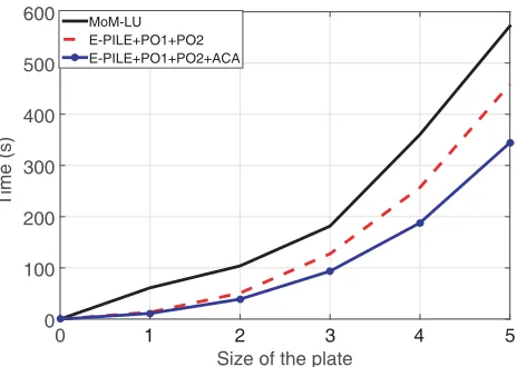
Figure 7. Comparison of time requires for the three methods, MoM-LU, E-PILE combined with PO and E-PILE combined with PO accelerated by ACA. The time is for scenario of square plate of dimensions from 1λ0×1λ0 to 5λ0×5λ0 and the rough surface is of dimension of 5λ0×5λ0.
of this paper. To verify this, we measure the time required for the MoM-LU, E-PILE+PO1+PO2, and E-PILE+PO1+PO2+ACA, and the simulations are launched several times. Then we take the average time needed. The computations are tested for a fixed size of rough surface of 5λ0×5λ0, then the size of the plate is changed from 1λ0×1λ0 to 5λ0×5λ0. Fig. 7 shows a comparison among the times required for the MoM-LU, E-PILE+PO1+PO2, and E-PILE+PO1+PO2+ACA.
From Fig. 7, we can notice that using the ACA allows us to reduce the computing time significantly. In a deeper look, at plate size of 5λ0 ACA approximately decreases the time 60 percent compared with the time MoM-LU takes. Also, the RCS from applying PO is almost the same as the RCS from PO combined with ACA, but the time used in PO combined with ACA is clearly less than the time used in PO only. The effect of ACA appears clearly for more geometry sizes where the unknowns are huge.
5. CONCLUSION
In this paper, an efficient hybrid method to study the electromagnetic scattering from a 3-D problem of two scatterers is presented. The method is based on the rigorous E-PILE method, originally developed to study the scattering for 2-D electromagnetic problems. A major advantage of the E-PILE method is that it can be combined with algorithms originally developed to solve problems of scattering from a single scatterer in free space. Consequently, the E-PILE method is combined with the PO approximation to calculate the local interactions on both the object and the rough surface. In this paper, the E-PILE+PO method is accelerated by using the ACA to accelerate the computation of the coupling matrices involved in E-PILE. As a result, the ACA method permits to strongly compress the coupling matrices without a loss of accuracy, so the memory requirement is strongly reduced.
REFERENCES
1. Guo, L.-X., A.-Q. Wang, and J. Wang, “Study on EM scattering from 2-D target above 1-D large scale rough surface with low grazing incidence by parallel MoM based on PC clusters,”Progress In Electromagnetics Research, Vol. 89, 149–166, 2009.
4. Dechamps, N., N. De Beaucoudrey, C. Bourlier, and S. Toutain, “Fast numerical method for electromagnetic scattering by rough layered interfaces: Propagation-inside-layer expansion method,”Journal of the Optical Society of America A, Vol. 23, No. 2, 359–369, 2006.
5. Kouali, M., G. Kubick, and C. Bourlier, “Electromagnetic scattering from two-scatterers using the extended propagation-inside-layer expansion method,” General Assembly and Scientific Symposium, 1–4, 2011.
6. Pino, M. R., F. Obelleiro, L. Landesa, and R. J. Burkholder, “Application of the fast multipole method to the generalized forward-backward iterative algorithm,”Microwave and Optical Technology Letters, Vol. 26, No. 2, 78–83, 2000.
7. Kubick, G. and C. Bourlier, “A fast hybrid method for scattering from a large object with dihedral effects above a large rough surface,” IEEE Transactions on Antennas and Propagation, Vol. 59, No. 2, 189–198, 2011.
8. Pino, M. R., L. Landesa, J. L. Rodriguez, F. Obelleiro, and R. J. Burkholder, “The generalized forward-backward method for analyzing the scattering from targets on ocean-like rough surfaces,” IEEE Transactions on Antennas and Propagation, Vol. 47, No. 6, 961–969, 1999.
9. Ye, H. and Y. Q. Jin, “Fast iterative approach to difference scattering from the target above a rough surface,” IEEE Transactions on Geoscience and Remote Sensing, Vol. 44, No. 1, 108–115, 2006.
10. Ye, H. and Y. Q. Jin, “A hybrid KAMoM algorithm for computation of scattering from a 3D PEC target above a dielectric rough surface,”Radio Science, Vol. 43, No. 3, 1–15, 2008.
11. Guan, B., J. F. Zhang, X. Y. Zhou, and T. J. Cui, “Electromagnetic scattering from objects above a rough surface using the method of moments with half-space Green’s function,”IEEE Transactions on Geoscience and Remote Sensing, Vol. 47, No. 10, 3399–3405, 2009.
12. Johnson, J. T., “A numerical study of scattering from an object above a rough surface,” IEEE Transactions on Antennas and Propagation, Vol. 50, No. 10, 1361–1367, 2002.
13. Johnson, J. T. and R. J. Burkholder, “Coupled canonical grid/discrete dipole approach for computing scattering from objects above or below a rough interface,” IEEE Transactions on Geoscience and Remote Sensing, Vol. 39, No. 6, 1214–1220, 2001.
14. Johnson, J. T., “A study of the four path model for scattering from an object above a half space,” Microwave and Optical Technology Letters, Vol. 20, No. 30, 130–134, 2001.
15. Guo, L. X., J. Li, and H. Zeng, “Bistatic scattering from a three-dimensional object above a two-dimensional randomly rough surface modeled with the parallel FDTD approach,”JOSA A, Vol. 26, No. 11, 2383–2392, 2009.
16. Kuang, L. and Y. Q. Jin, “Bistatic scattering from a three-dimensional object over a randomly rough surface using the FDTD algorithm,” IEEE Transactions on Antennas and Propagation, Vol. 55, No. 8, 2302–2312, 2007.
17. Kouali, M., G. Kubick, and C. Bourlier, “Extended propagation-inside-layer expansion method combined with the forward-backward method to study the scattering from an object above a rough surface,” Optics Letters, Vol. 37, No. 14, 2985–2987, 2012.
18. Boag, A. and R. Mittra, “Complex multipole beam approach to electromagnetic scattering problems,” IEEE Transactions on Antennas and Propagation, Vol. 42, No. 3, 366–372, 1994. 19. Tap, K., P. H. Pathak, and R. J. Burkholder, “Complex source beam-moment method procedure
for accelerating numerical integral equation solutions of radiation and scattering problems,”IEEE Transactions on Antennas and Propagation, Vol. 62, No. 4, 2052–2062, 2014.
20. Canning, F. X., “The impedance matrix localization (IML) method for moment-method calculations,” IEEE Antennas and Propagation Magazine, Vol. 32, No. 5, 18–30, 1990.
21. Zhao, K., M. N. Vouvakis, and J. F. Lee, “The adaptive cross approximation algorithm for accelerated method of moments computations of EMC problems,” IEEE Transactions on Electromagnetic Compatibility, Vol. 47, No. 4, 763–773, 2005.
Progress In Electromagnetics Research M, Vol. 37, 175–182, 2014.
23. Yang, W. and C. Qi, “A bi-iteration model for electromagnetic scattering from a 3D object above a 2D rough surface,”Electromagnetics, Vol. 35, No. 3, 190–204, 2015.
24. Kouali, M., G. Kubick, and C. Bourlier, “Scattering from an object above a rough surface using the extended PILE method hybridized with PO approximation,” Antennas and Propagation Society International Symposium (APSURSI), 1–2, 2012.