MAKUENI COUNTY, KENYA.
By
PIUS MWENDA BORONA Reg No. N50/25774/2011
A Thesis submitted in Partial Fulfillment of the Requirements for the award of Degree of Master of Environmental Science in the School of Environmental Studies
of Kenyatta University
Declaration
Declaration by candidate:
This thesis is my original work and has not been presented for a degree in any other University or other award
Signature...Date....8/1/2016... Pius Mwenda Borona
N50/25774/2011
Department of Environmental science Kenyatta University.
Declaration by Supervisors
We confirm that the work reported in this thesis was carried out by the student under our supervision
Signature... Date... Prof.James Biu Kung’u (PhD)
Department of Environmental Science Kenyatta University
Signature... Date... Dr.Dionysious Kiambi
Dedication
Acknowledgement
I wish to express my deepest gratitude to several persons who provided me with technical, emotional and financial support through the documentation of this work.
Notably, my first supervisor Prof.James Biu Kung’u for his guidance from proposal defense to defense of results all aiming at coming up with publishable material.
I additionally wish to mention my second supervisor Dr.Dionysious Kiambi’s invaluable technical guidance, through Africa Biodiversity Conservation and Innovations Center (ABCIC), in documentation and more so financial support throughout the research. In addition I wish to thank Bioversity International staff, for their instrumental input through the CCAFS programme.
TABLE OF CONTENTS
DECLARATION ... i
DEDICATION ... ii
ACKNOWLEDGEMENT ... iii
LIST OF TABLES ... viii
LIST OF FIGURES ... x
LIST OF PLATES ... xi
ABBREVIATIONS AND ACRONYMS ... xii
ABSTRACT...xiv
CHAPTER ONE: INTRODUCTION ... 1
1.1 Background of the study ... 1
1.2 Problem Statement ... 4
1.3 Justification ... 5
1.4 Research Questions ... 5
1.5 Objectives ... 6
1.5.1 Main Objective... 6
1.5.2 Specific Objectives ... 6
1.6 Research Hypotheses ... 6
1.7 Significance... 7
1.8 Conceptual Framework ... 8
1.9 Definition of Key Terms ... 10
1.10 Assumptions and Limitations ... 11
CHAPTER TWO LITERATURE REVIEW ... 12
2.1 Introduction ... 12
2.2 Causes of climate change and climate variability ... 12
2.3 Global, regional and local Climate change projections ... 13
2.4 Impacts of Climate variability and change on Agriculture and livelihoods ... 14
2.5 Specific impacts associated with climate change and variability in semi-arid agroecosystems and the importance of adaptations. ... 15
2.6 Climate change tolerance and the focus crops ... 17
2.8 Literature gaps on vulnerability to climate change ... 19
CHAPTER THREE: METHODOLOGY ... 21
3.1 Introduction ... 21
3.2 The study area ... 21
3.3 Description of Study Area ... 22
3.4 Sample Size and Sampling techniques ... 23
3.5 Research Instruments ... 24
3.5.1Data Collection ... 24
3.5.1.1Secondary data ... 24
3.5.1.2 Primary data ... 25
3.5.2 Data management and analysis techniques ... 26
3.5.3 Validity and Reliability ... 33
CHAPTER FOUR: RESULTS AND DISCUSSION ... 34
4.1 Introduction ... 34
4.2 Household socio economic characteristics ... 34
4.2.1 Respondents gender and Age ... 34
4.2.2 Household roles ... 36
4.2.3 Education levels ... 37
4.2.4 Household size ... 39
4.2.5 Main occupation and Income sources ... 40
4.2.6 Livestock assets ... 46
4.2.7 Land ownership ... 49
4.3 Exposure context-Indicators of climate events affecting households. ... 55
4.3.1 Key Climate Indicators ... 55
4.3.2 Perceptions on direction of change of weather and related parameters ... 62
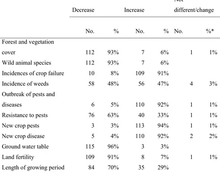
4.3.3 Patterns of selected ecosystem based variables in the last 10 years ... 67
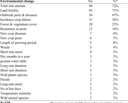
4.3.4 Significant climatic and non-climatic changes over the last ten years in Wote 70 4.3.5 Trend analysis of climate data from 1983 to 2013, for Wote ... 73
4.3.5.1 Annual temperature and precipitation trends ... 73
4.3.5.2 Seasonal trend analysis ... 75
4.4 Climate Change and variability Impacts in Wote ... 80
4.4.1 Impacts associated with drought in Wote ... 80
4.4.3 Impacts associated with erratic rains in Wote... 83
4.4.4 Impacts associated strong winds in Wote ... 86
4.4.5 Impacts associated with crop pests and diseases in Wote... 88
4.4.6 Hypotheses test results ... 90
4.5 Adaptation strategies ... 92
4.5.1 Adaptations to major calamities... 92
4.5.1.1 Adaptations to drought in Wote ... 92
4.5.2.2 Adaptation to erratic rains in Wote ... 96
4.5.2.3 Adaptations to Strong winds in Wote ... 97
4.5.2.4 Adaptations to crop pests and diseases in Wote ... 98
4.5.3 Adaptations to major changes in land and natural environment ... 101
4.5.3.1 Adaptations to changes in land fertility in Wote ... 101
4.5.3.2 Adaptations to vegetative cover changes in Wote ... 103
4.5.4 Access to weather and calamities information as an adaptation mechanism . 105 4.5.5 Selected adaptation mechanisms ... 111
4.6 Socioeconomic factors influencing adaptation in Wote ... 118
4.6.2 The relationship between adaptations and socio economic factors in Wote .. 119
4.7 Vulnerability context of Wote Households... 136
4.7.1 Vulnerability context among Wote households ... 136
4.7.2 Hypotheses test results ... 143
CHAPTER FIVE: CONCLUSIONS AND RECOMMENDATIONS ... 145
5.1 Summary ... 145
5.2 Conclusions ... 148
5.3 Recommendations ... 150
6.0 REFERENCES ... 152
7.0APPENDICES...166
Appendix 1 Household size statistics ... 166
Appendix 2 Additional monthly income statistics ... 166
Appendix 4 Food insecurity statistics ... 167
Appendix 5 Correlation Matrix for testing multicollinearity in the multiple linear regression model. ... 168
Appendix 6 Multiple regression model coefficients complete table ... 170
Appendix 7 Observation checklist ... 171
List of Tables
Table 4.1 Gender distribution of main respondent and correspondent in Wote ... 34
Table 4. 2 Age distribution statistics of the respondents ... 35
Table 4.3 Age distribution of main respondents correspondents in categories in Wote .. 36
Table 4.4 Roles of main and correspondents in Wote ... 37
Table 4.5 Education level of Respondents in Wote ... 38
Table 4.6 Household size categories ... 39
Table 4.7 Main occupation of respondents in Wote ... 41
Table 4.8 Main Household income sources among Wote Households ... 42
Table 4.9 Main Income sources among households in Wote ranked ... 44
Table 4.10 Cash Income categories among Wote Households ... 45
Table 4.11 Respondent ownership of specific livestock ... 46
Table 4.12 Plot ownership/tenure among households in Wote... 49
Table 4.13 Acreage statistics of Wote Households ... 51
Table 4.14 Test for acreage Normality of Wote households land acarage ... 51
Table 4. 15 Plot orientation of households land, Wote ... 53
Table 4. 16 Key calamities experienced by households in Wote ... 55
Table 4.17 Cross tabulation of multiple calamities experienced by households in Wote 56 Table 4. 18 Major calamities in the last fifty years at the community level ,Wote ... 58
Table 4.19 Recent occurrences of drought events in Kenya from 1980 to 2011 ... 60
Table 4.20 Ranking of Key calamities experienced by households in Wote ... 61
Table 4.21 Kendall’s coefficient of concordance for key calamities ranking ... 62
Table 4.22 Perception on selected weather parameters comparing with 10 years ago ... 63
Table 4.23 Households perception on Changes in selected weather parameters over the last 10 years in Wote ... 63
Table 4.24 Responses on changes in selected parameters over the last decade in Wote .. 67
Table 4.25 Most significant weather and related changes by count experienced by households in Wote ... 71
Table 4.26 Annual average temperature trend statistics for Wote ... 74
Table 4.27 Coefficients of variation for short and long rains for Wote ... 76
Table 4.28 MMM season statistics for Wote for the period 1977 to 2013 ... 77
Table 4.29 Statistics for OND season in Wote for the period 1977 to 2013 ... 78
Table 4.30 Key impacts experienced as a result of drought in Wote households ... 80
Table 4.31 Key impacts associated with erratic rains in Wote ... 84
Table 4.32 Impacts associated with strong winds in Wote ... 86
Table 4. 33 Impacts associated with crop diseases in Wote ... 88
Table 4.34 Impacts associated with crop pests in Wote ... 89
Table 4.35 Hypothesis summary for the relationship for the relationship between key extreme events and crop failure (Chi square test) ... 91
Table 4.37 Drought adaptation mechanisms among households in Wote ... 92
Table 4.38 Adaptations to erratic rains among households in Wote ... 96
Table 4.39 Adaptation to strong winds among households in Wote ... 98
Table 4.40 Adaptation to crop pests among households in Wote ... 99
Table 4.41 Adaptations to crop diseases among households in Wote ... 100
Table 4.42 Adaptations to land fertility loss among households in Wote ... 101
Table 4.43 Adaptation to vegetative cover change among households in Wote ... 104
Table 4.44 Households indication of weather information importance in Wote ... 106
Table 4.45 Most important weather information ranking in Wote ... 106
Table 4.46 Weather and calamities information received in the last two years in Wote 108 Table 4.47 Main weather and calamity information sources in Wote ... 109
Table 4.48 Selected adaptation mechanisms among Households in Wote ... 111
Table 4.49 Total number of adaptations to calamities experienced in Wote ... 119
Table 4.50 Regression model summary ... 120
Table 4.51 Statistics for continuous variables included in the linear regression model . 122 Table 4.52 Collinearity statistics for the multiple regression model ... 126
Table 4.53 Residual statistics for the multiple regression model ... 127
Table 4.54 Model fitting statistics summary... 131
Table 4.55 ANOVA table showing model significance ... 132
Table 4.56 Summary of the multiple regression model coefficients table ... 133
Table 4.57 Distribution of monthly food insecurity among the Wote households ... 136
Table 4.58 Distribution of monthly food shortage within a year in Wote ... 136
Table 4.59 Hypothesis summary for occupation of main respondent against food security ... 143
List of Figures
Figure 1.1 Conceptual framework...8
Figure 3.1 Map of the Study Area...23
Figure 4.1 Number of owned plots among households in Wote... 49
Figure 4.2 Quartile (Q-Q) Plot for testing acreage distribution in Wote ... 52
Figure 4. 3 Annual temperature trends-1983 to 2011 for Wote ... 74
Figure 4.4 Annual precipitation trends-1983 to 2012 for Wote ... 75
Figure 4. 5 Standardized anomaly indices for seasonal rainfall 1977 to 2013 in Wote ... 76
Figure 4. 6 Reasons and benefits for adoption of selected adaptation strategies among Households in Wote ... 112
Figure 4.7 Scatter plot of the Linear relationship between studentized residuals and unstandardized predicted value ... 121
Figure 4. 8 Linear relationship between transformed studentized residuals and unstandardized predicted value ... 123
Figure 4. 9 Partial regression plots for main respondent’s age. ... 123
Figure 4.10 Partial regression plots for household number ... 124
Figure4. 11 Partial regression plots for mean acreage ... 124
Figure 4.12 Partial regression plots for correspondent’s age ... 125
Figure 4.13 Superimposed curve for detecting normality among transformed predictors... 128
Figure 4.14 Detecting normality after transformation of predictors ... 128
Figure 4.15 Plot for checking non-violation of homogeneity of variances ... 130
List of Plates
ABBREVIATIONS AND ACRONYMS
ASALs Arid and Semi-Arid Lands
ASARECA Association for Strengthening Agricultural Research in East and Central Africa
ATPS Africa Technology and Policy Studies Network
CCAFS Climate change agriculture and food security research project (under the CGIAR consortium)
CGIAR Consultative Group for International Agricultural Research CSTI Center for Science Technology and Innovation
ENSO Elnino southern oscillation
FAO Food and Agricultural Organization FGD Focus Group Discussion
GDP Gross Domestic Product
GIS Geographical Information System
IARSAF International Association of Research Scholars and Fellows IASC International arctic science committee
ICPAC IGAD Climate Prediction and Application Center
ICRISAT International Crop Research Institute for Semi-Arid Tropics IFC International Finance Corporation
IGAD Inter-Governmental Authority on Development IISD International Institute of Sustainable Development IITA International Institute of Tropical Agriculture ILRI International Livestock Research Institute IPCC Intergovernmental Panel on Climate Change
KNBS Kenya National Bureau of Statistics LVBC Lake Victoria Basin Commission MDGs Millennium Development Goals
MoAL Ministry Of State for Development of Northern Kenya and Other Arid Lands
MoE Ministry of Environment
NIACS National Institute of Applied Climate Science
NWCPC National Water Conservation and Pipeline Corporation PANESA Pastures Network for Eastern and Southern Africa PWC Price Waterhouse Coopers
SFSU San Francisco State University SMEs Small and Medium Enterprises SSA Sub Sahara Africa
SACCO Savings and Credit Cooperative Society
UNCTAD United Nations Conference for Trade and Development UNEP United Nations Environmental Programme
ABSTRACT
Climate variability and change are some of the most pressing environmental challenges of the globe and are associated with complexity and extreme events mainly drought and floods. Among small scale farming communities in Sub-Saharan Africa including Kenya, climate variability and change have been a more tasking challenge compared to the rest of the regions. There is little understanding of the vulnerability to climate change among such households in Wote based on their socio economic backgrounds. The main objective of the study was to determine the extent of vulnerability among small scale farmers in Wote division, Makueni County by specifically determining exposure, sensitivity and adaptation mechanisms as pertains climate extremes. The study was carried out between August and September 2013. The study targeted selected farmers cultivating drought tolerant sorghum, cow peas and pigeon peas which are some of the dominant multipurpose crops in the area and are also key means of food security. Random and purposive sampling methods were applied in identifying households cultivating all the three focus crops. Data collection methods and sources included the use of focused group discussions, semi structured questionnaires and secondary climate data from the meteorological department. The collected data was entered and cleaned using CSPro program and later exported to Ms Excel and SPSS for coding and analysis. Descriptive and inferential statistics approaches included correlation, chi square, non-parametric tests and regression. Household characteristics included main respondents and correspondents, 86% and 76% respectively, engaging in farming as the main occupation with 86% of household’s main income obtained from on farm produce. Results showed that households have been exposed to calamities in form of; drought, 100%: crop pests, 93%: crop diseases, 83% and erratic rains, 59% with drought ranking highly ( =1.06,=0.28).Crop diseases significantly related to occurrence of crop failure,2=24.860,p=0.000 and Cohen’s index=0.445 showing a medium relationship.
Drought however did not show a significant relationship with crop failure,
p=0.334.Temperature data indicated an annual trend of 0.21220C (R2=0.4881) per year
CHAPTER ONE: INTRODUCTION
1.1 Background of the study
Climate change, as defined by the IPCC, refers to “statistically significant variation in either the mean state of the climate or its variability, persisting for an extended period typically decades or longer” (IPCC, 2001a). The UNFCCC distinguishes climate change and climate variability with the former being associated with anthropogenic activities such as land use change leading to alteration of the atmospheric composition: the latter is linked to natural processes (UNFCCC, 2014) including SST changes (Lyon & DeWitt, 2012) in the tropical Atlantic and Indian ocean (Johnson, 1996). In addition the WMO give a wider definition of climate variability as “variations in the mean state and other statistics of climate on temporal and spatial scales beyond individual weather events”(WMO, 2015).
Climate variability and change have been identified as major challenges facing communities at local, regional and international levels in an array of ways such as prolonged drought and flooding (LVBC, 2011). Indeed data for the last 100 years indicates that the climate over the African continent has warmed up (Hulme, et al., 2001). Hulme et al., (2001) add that this warming has severe impacts on the available water resources an effect that is anticipated regardless of significant alteration of future rainfall. High confidence IPCC projections further indicate that climate change will amplify existing stress on available and already stressed water resource catchments in Africa (Niang et al., 2014).
Effects of extreme events resulting from climate change are becoming a major area of concern and will affect the poor in developing countries in many ways (Desanker & Justice, 2001) including amplifying poverty levels (Speranza et al., 2010). High confidence projections by the IPCC in the fifth assessment outline that climate change will interact with non-climatic drivers to amplify vulnerability of agricultural systems especially in semi-arid areas (Niang, et al., 2014). Specifically, changes in rainfall and temperature are likely to lead to drop in cereal yields quantity and quality which will have severe effects on food security.
The IPCC assessment as detailed by Niang et al., (2014) indicates that climate change is likely to amplify existing health challenges in the Africa region for example highlands of East Africa could start experiencing instances of malaria including increased health risks as a consequence of insufficient safe water, poor sanitation and limited access to health care.
Vigna ungucuilata (Cowpeas), Cajanus cajan (Pigeon peas) and Sorghum bicolor
(Sorghum) (referred to as, focus crops, hereafter) are examples of drought tolerant crops and their varieties widely cultivated by small scale farmers in Wote (RoK, 2013). There are renewed efforts, including cutting edge research, to enhance cultivation of the focus crops in SSA to enhance adaptive capacity among these farmers such that they benefit from their efforts (CGIAR, 2006; IITA, 2009; ICRISAT, 2014). The focus crops farmers were the entry point of this study since understanding multiple risks posed among these farmers is going to inform appropriate and transferable adaptive capacities.
1.2 Problem Statement
There is evidently little understanding of the drivers and nature of vulnerability of such communities and households in this Semi-arid area. The need to identify indicators of vulnerability to inform on the best interventions to enhance existing adaptive capacity and even transfer and share adaptation mechanisms, informed this study.
1.3 Justification
Enhancement of adaptive capacity among Wote small scale farmers cultivating the drought tolerant focus crops is necessary to enhance resilience at the local level. This is primarily because the farmers in Wote, which is largely semi-arid, are heavily dependent on rain fed farming and are frequently exposed to instances of extreme climate events such as intermittent rainfall. Appropriate and informed crop based adaptation mechanisms and related response strategies indeed do assist small scale farmers achieve food, income and livelihood security in the face of climate variability and change. Accordingly, this research was critical in characterizing the nature and drivers of vulnerability among Wote small scale farmers, cultivating the drought tolerant focus crops, based on their socio economic profiles and acclimatization means. The study is equally essential to inform on appropriate interventions for buffering against inherent and new combinations of climate extremes.
1.4 Research Questions
1. Which are the socio-economic characteristics of the focus crops small scale farmers in the Wote area affecting their adaptation to climate change?
3. How is climate variability and change affecting livelihoods of the focus crops small scale farmers in the study area?
4. Which similar or different means of adaptation have the focus crop small scale farmers in the study area applied with regard to climate variability and change? 5. How vulnerable are the focus crop small scale farmers in the study area?
1.5 Objectives 1.5.1 Main Objective
The main objective of the study was to assess the extent to which the small scale focus crops cultivating households in Wote are vulnerable to prevailing climate variability and change conditions.
1.5.2 Specific Objectives
1. To determine the socio-economic factors that influences the focus crops small scale farmers’ adaptation to climate change and variability in Wote areas.
2. To identify local climate variability and change indicators that are affecting the focus crops small scale farmers in Wote area.
3. To examine the impacts of climate variability and change indicators on livelihoods of the focus crops small scale farmers in the study area.
4. To characterize the existing adaptation strategies among the focus crop small scale farmers in the study area.
5. To determine the extent of vulnerability among the focus crop small scale farmers in the study area.
1.6 Research Hypotheses
i) There is a significant relationship between extreme events and crop failure. ii) Key occupation of the small scale farmers significantly influences their food
security.
iii) There is a significant relationship between food insecurity (number of food short months) and the aggregated household income.
1.7 Significance
1.8 Conceptual Framework
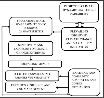
Climate change vulnerability is a relationship between exposure to climate variations, sensitivity to the stressors and adaptive capacity of the households (Schneider et al., 2001; Adger & Vincent, 2005). An example is as Sanchez (2000) state, agricultural vulnerability to climate change and variability effects can be detailed in terms of exposure to elevated temperatures, crop yield sensitivity and the ability of farmers to adapt to extremes. Figure 1.1 outlines the relationship between the discussed climate change vulnerability variables linked to specific objectives and data collection tools.
PREVAILING /OBSERVED CLIMATE CHANGE AND VARIABILITY INDICATORS SENSITIVITY AND
EXPOSURE TO CLIMATE CHANGE EXTREMES FOCUS CROPS SMALL SCALE FARMERS SOCIO
ECONOMIC CHARACTERISTICS PROJECTED CLIMATE DYNAMICS INCLUDING VARIABILITY PREVAILING IMPACTS HOUSEHOLD AND COMMUNITY ADAPTATION AND COPING MECHANISMS FOCUS CROPS SMALL SCALE
FARMERS VULNERABILITY SENSITIVITY AND EXPOSURE TO CLIMATE
CHANGE EXTREMES PREVAILING /OBSERVED CLIMATE CHANGE AND VARIABILITY INDICATORS
Figure 1.1Conceptual framework adapted from (Füssel & Klein, 2006; NIACS, 2012) showing the relationship between key variables explaining vulnerability.
The vulnerability assessment initially sought to capture selected socio economic characteristics of the focus crops small scale farmers at household levels in Wote that could influence sensitivity and adaptive capacity. Exposure sought to identify specific extreme events including droughts and strong winds that have been experienced by the small scale farmers cultivating the focus crops, including reference to available projections by the IPCC and meteorological data from the Kenya meteorological department.
Impacts include effects associated with exposure to extreme climate events that the households have experienced. Sensitivity to climate extremes is as a result of exposure to extremes and the extent is captured with reference to socio economic profiles (Heltberg et al., 2009). Adaptive capacity is captured as the various adaptation strategies that households have put in place and the availability of government and non-government agencies assistance to farmers when climate extremes strike. These adaptation mechanisms reduce the vulnerability of farmers or in other cases fail to absorb or manage experienced risks. These mechanisms are linked to the socio economic profile of the households including the level of income and the level of education.
1.9 Definition of Key Terms
Exposure-defined as the direct stressor and the extent of climate impacts either short or long term on a particular system and includes changes in climate variability and magnitude or frequency of extreme events.
Sensitivity- extent to which a natural or social system will respond to a particular change or variability in climate whether beneficial or harmful. Sensitivity can also be defined as environmental and human conditions that increase, worsen or trigger impacts.
Adaptation-defined as adjustments in practices, processes or structures to offset or accrue from climate variability and change and can be planned or autonomous.
Risk- Probability of damage, liability or injury or equivalent negative occurrence that results from either external or internal vulnerabilities.
Livelihood-array of on-farm and off-farm activities that provide that involve an array of means for making a living
Food security-refers to a state of people’s capacity to access safe, adequate and nutritious food.
Focus crops-A word used in this documentation to refer to crops of interest in this research; Sorghum, Cowpeas and Pigeon peas and hence associated households.
Respondent- In this analysis this refers to the household head involved in making of key household decisions and is the main provider of household income.
1.10 Assumptions and Limitations
It was expected that all respondents will cooperate during the data collection exercise and data collection tools would be well understood. The assumption was indeed met as an array of quality control measures were applied during the study. This included re visiting selected households, while in the field, where provided data had some inconsistencies. The weather and transport network at the proposed study time was expected to be serene. Indeed the weather was friendly hence challenges of accessing farmer’s locations/households were not experienced.
CHAPTER TWO LITERATURE REVIEW
2.1 Introduction
This chapter discusses the aspect of climate change and variability including global, regional and local climate change predictions as well as aspects of climate impacts and adaptation. Further, the chapter discusses the relationship between the focus crops of the study and climate change extremes. The chapter then presents related research on climate change vulnerability while outlining gaps in such research.
2.2 Causes of climate change and climate variability
Research indicates that key factors bringing about changes in the earth’s energy balance and subsequent climate change include; changes in the abundance of greenhouse gases, cloudiness and aerosols, alteration of the earth’s atmosphere and surface reflectivity (Forster et al., 2007; IPCC, 2007). The release of GHGs, has been shown since mid-18th century; tended to significantly bring about a warming effect on the earth as a result of alteration of the abundance and properties of GHGs in the atmosphere (Baede et al., 2001). Agriculture contributes about 13.5% of global GHGs emissions mainly methane and nitrous oxide, representing 47% and 58% of the total CH4 and N2O respectively: such
2.3 Global, regional and local Climate change projections
Climate change projections by computer models foresee a global average temperature increase of 0.10C per decade with global mean surface temperature increase of between 1.50C and 5.80C by the year 2100 (Folland et al., 2001; IPCC, 2007; Chidumayo, et al., 2011).
Generally with such temperature rises projections indicate occurrence of key extreme events such as; more frequent heat waves, decrease in (diurnal) temperature range, fewer frost days(in north and central Europe), decrease in frequency of cold air outbreaks, summer dryness/dry extremes and winter wetness-or both at the same place, intense precipitation (due to warmer atmosphere) (Folland, et al., 2001; FAO, 2012).
The most important elements of climate change in Africa include variations in precipitation, occurrence of extreme events as well as CO2 enrichment (Downing et al.,
Projections for Kenya to the 2030’s indicate a temperature increase trend of a maximum of about 30C with regions extending from Lake Victoria to the east of Kenya’s central highlands expecting increases in rainfall with maximums at 20% (MoE, 2002).
2.4 Impacts of Climate variability and change on Agriculture and livelihoods
Significant impacts of climate variability and change on agriculture include raising the water demand, limiting crop productivity and reducing water availability where irrigation is needed, increased pest attacks and reduced soil fertility (Chidumayo, et al., 2011; FAO, 2012). In the mid to higher latitudes, a rise in temperature of between 2-30C and higher CO2 levels is likely to benefit- with adaptation-due to lengthening of the growing season
(Stern, 2006; Easterling et al., 2007; FAO, 2012) . High confidence projections for Africa by the IPCC indeed indicate ecosystems including species shifts, amplification of water stress, reduced cereal production and increased diseases prevalence (Niang, et al., 2014). These impacts are expected to lead to other devastating effects including effects on fisheries, slowed economic development due to water scarcity and food insecurity and high infant mortality coupled with malnutrition. Niang et al., (2014) emphasize that semi-arid regions are likely to experience severer impacts due to additional influence by non-climatic drivers and stressors and these effects will largely alter agricultural ecosystems subsequently leading to food shortage. This shortage includes aspects of food security such as availability, access, utilization and price stability (Porter et al., 2014).
These key impacts are largely associated with changes and variations in temperature and precipitation. An estimate of economic costs by Heinrich-Boll-Stiftung (2013) indicates annual losses of about $0.5billion annually from continued extreme climate events in Kenya. Wote area being classified as semi-arid is similarly vulnerable to more frequent severe droughts which are mainly characterized by long dry spells and water shortage (MoE, 2002; Rao, et al., 2011; RoK, 2013).
2.5 Specific impacts associated with climate change and variability in semi-arid agroecosystems and the importance of adaptations.
Climate change and variability are mainly associated with instances of dry spells and droughts which principally result from highly variable rainfall and high temperatures. Dry spells are lengthy instances of absence of rainfall during the growing period which grow into droughts when this length is about 40 days (Mkandawire, 2014) . As such dry spells play a role in shortening of the growing season by bring about a delayed or false onset of the season. Subsequently, there is a high likelihood of crop failure as well as inter-annual yield variability especially for moisture dependent cereals such as maize (Kambire et al., 2010). Instances of dry spells in arid environments indeed largely influence soil-moisture availability (Kisaka et al., 2015) and subsequently contribute to crop-water deficit during key crop growth stages (Igbadun et al., 2005).
Vulnerability assessments in other areas have indeed noted the importance of livestock as a key income generating activity (IGA) where such livestock is traded in markets (LVBC, 2011; Recha, 2011). Being a key livelihood sources, including provision of nutrition, livestock loss due to extreme climate events could greatly increase the vulnerability of small holder households.
In the event of climate change and variability impacts as well as changes in socio economic conditions, farming communities at individual level employ adjustments or adaptations to manage associated impacts. These practices also aim at taking advantage of new opportunities. These adjustments can reduce the unforeseen damage resulting from extreme weather risks and are important in Africa where there is higher vulnerability coupled with lower adaptive capacity (Hassan & Nhemachena, 2008). These adaptations assist small holder households achieve their food, livelihood and income security in the face of climate risks and non-climatic drivers such as market fluctuations (Kandlikar & Risbey, 2000). Adger et al., (2003) in their review outline that many adaptation efforts in developing countries will be informed by past experiences and will be further autonomous and facilitated by their own social capital and resource base.
This implies certain socio economic factors influence the nature and choice of adaptation mechanisms that a household employs (Deressa et al., 2009) with certain adaption mechanisms proving beneficial in addressing climate impacts while others fail (Porter, et al., 2014). Adger et al., (2009) in their detailed review emphasize that a wide range of factors including knowledge on future climate, ethics and their manifestation as well as the value given to places and cultures equally influence climate notwithstanding physical and ecological barriers. This aspect is further reiterated by Kandlikar & Risbey, (2000) who indicate that infrastructure, information systems as well as research for development equally play a role in enhancing adaptation. Absence of these mechanisms in developing countries amplifies their vulnerability.
As such while adaptation mechanisms remain the key drivers of addressing climate induced risks among many households in rural areas of SSA, there are combinations of forces that hinder these resilience efforts, subsequently increasing household’s vulnerability. These forces range from those occurring at the household and community level to those manifested at the national and regional stage.
2.6 Climate change tolerance and the focus crops
Cowpeas is the most grown grain in the dry areas of Africa producing (5.2 million tons) since the legume tolerates drought and performs in a wide array of soils (IITA, 2009). The cereal is preferred because of its adaptation to marginal climate and suitability for intercropping systems and fast maturity (Infonet-Biovision, 2015a). Pigeon pea is an important crop in Kenya and is grown for home consumption and export and is also rain fed (ICRISAT, 2014). It is an important grain legume in the rain fed farming of semi-arid tropics and yields well in drier conditions with poor soil quality while offering high protein content (Cook et al., 2005; ICRISAT, 2014) . The legume is also used for other purposes such as livestock feed as well as firewood as well as wind control (Cook, et al., 2005).
Sorghum is the fifth most important multipurpose cereal grown in 105 African countries with sweet sorghum providing food, feed, fuel and fodder without significant tradeoffs in grain production (ICRISAT, 2014). Sorghum has a wide adaptability, has a high levels of iron and zinc and is drought hardy than maize but is affected by sustained flooding and numerous diseases (ICRISAT, 2014). Other than tolerating drought conditions the crop also tolerates a wide range of soil types including poor soils where other crops fail (Infonet-Biovision, 2015b).
2.7 Climate change vulnerability assessment
Recent research on effects of climate variability and change has led to development of the concept of vulnerability to climate change. This refers to the probability to which a natural, social system or wellbeing is susceptible to adapt to or recover from effects resulting from climate change (Kelly & Adger, 2000; Schneider, et al., 2001). Further, three important components are applied in understanding the concept of vulnerability in sectors such as agriculture including: sensitivity, exposure and adaptive capacity (Schneider, et al., 2001; Adger & Vincent, 2005; Easterling, et al., 2007; Heltberg, et al., 2009).
Assessing or rather assessment of vulnerability to climate variability and change seeks to understand which socioeconomic groups or regions are at risk, how and why they are susceptible (Ribot, 1996). Vulnerability assessments present a useful tool for comprehending and responding via appropriate adjustments at national and community levels though there exists challenges such as scarcity of data, crosscutting stressors (non-climate linked) and limited capacity especially in Africa (Adger & Vincent, 2005; Nzeh & Eboh, 2011).
2.8 Literature gaps on vulnerability to climate change
In addition this study emphasizes on the identified gaps in understanding vulnerability based on socio-economic dimensions at household level as several of reviewed studies on vulnerability emphasize. For example this study looks at vulnerability from a multidimensional point of view by use of socio-economic data and meteorological data. The study additionally involves research at local levels to capture specific social dimensions of climate change. Further the study addresses the gap in understanding vulnerability by emphasizing on socio-economic profiles unlike the use of secondary data. This brings out the local focus in understanding vulnerability.
CHAPTER THREE: METHODOLOGY
3.1 Introduction
This chapter includes a description of the study areas geography, population, climate and administrative location. The chapter also discusses the selection of the study area in relation to the continuing project linked to this study. In addition the details on the sampling strategy, research instruments and data analysis are discussed.
3.2 The study area
The study was part of an ongoing project (CCAFS) which cut across the CGIAR consortium, also reported by other studies within the project (Rufino et al., 2013a). The criterion for selection of the study area: heavily applied GIS and remote sensing (high resolution images) and ground truthing techniques to identify dominant production systems -while relying on secondary and primary data: has been detailed below (CGIAR-CCAFS, 2011; Rufino et al., 2013b).
The larger sites (regions), e.g. East Africa in this case, were selected referring to the factors; “There is poverty and high degree of vulnerability to climate; significant but contrasting climate related problems and opportunities for intervention; security, governance, institutional capacity that favour likelihood of generating transferable results; complementary climatic contexts and reflecting different temporal and spatial scales of climate variability and predictability”.
The blocks are within larger sites (regions) and are chosen where the site listed selection criteria are met which include exhibiting variation with blocks in other regions. Further, benchmark sites or blocks identified within the regions are areas experiencing drier and wetter areas or are at high risk of climate change effects; Wote is associated with severe drought (CGIAR-CCAFS, 2013). The benchmark sites are also focal locations that are expected to generate results that can be applied and adapted to other regions worldwide since these sites are also broad areas including several adjacent districts.
3.3 Description of Study Area
The Wote site (Plate 3.1) lies in Makueni constituency/sub county (RoK, 2013) which has a population of about 243,219 and about 50,203 households and lies within Makueni County in lower eastern Kenya (KNBS, 2011). The coordinates of the specific sampling block are: 370.378E, 10.657S; 370.298E, 10.702S; 370.244E, 10.624S; 370.326E, 10.581S as shown in the map (Figure 3.1) (Wiebke et al., 2011).
Figure 3.1 Map of the study area
The mean temperature range is between 20.20C and 24.60C and is characterized by extreme rainfall variability which affects farming. Hilly areas receive about 800-1200mm per annum while the rest of the areas receive about 500mm per annum. The existing community practices mainly small scale rain fed Agriculture and livestock rearing.
3.4 Sample Size and Sampling techniques
In the ILRI-CCAFS sample, 10 villages were randomly selected within each of the two systems and subsequent random selection of ten households in each of the sampled villages. In the listing of villages and households, local leaders notably elders and chiefs were involved mainly in identification of persons and boundaries.
Households cultivating all the three focus crops, were selected by purposive sampling., A total of 120 households cultivating all the three focus crops (sorghum,cowpeas and pigeonpeas) were purposively selected from the ILRI-CCAFS sample.
3.5 Research Instruments
3.5.1Data Collection
A one week pretesting of the research instruments was carried out in the month of July 2013. Both primary and secondary data were collected between the months of August and September 2013.
3.5.1.1Secondary data
3.5.1.2 Primary data 1. Questionnaires
This included use of pretested questionnaires (Appendix 9) which were semi structured and coded and targeted household respondents for quantitative and qualitative data.
The questionnaire also included measures such as Likert scales. The likert scale was chosen since it has an array of merits and is one of the most common attitude or level of agreement to statement scales (Monette et al., 2013). Merits of likert scales include; possibility of identifying differences among respondents and gives respondents an array of choices and further provides ordinal data that can be analyzed using powerful statistics than nominal data (Kothari, 2011; Monette, et al., 2013). The aim was to capture socio economic data, adaptation strategies, climate impacts and perceptions on climate change.
2. Focus group discussion(FGD)
These targeted knowledgeable focus crops farmers in the study areas focusing on vulnerability to climate variability and change at the community level and sought quantitative data to supplement survey data.
These tool captured aspects such as perceptions on climate change and adaptation at community level. The Focus Group Discussions (Appendix 10) selected men and women from across the villages. The listed villages in the study area were randomly selected and knowledgeable and active farmers nominated from sampled villages with the assistance of local leaders.
3. Observation
Direct field observations and photography were applied to identify adaptation strategies and GPS readings of all households were recorded. This was to mainly capture photographic records of specific indicators of socio economic profile and adaptation strategies. An observation checklist (Appendix 7) was applied in this study.
3.5.2 Data management and analysis techniques
Air temperature and precipitation are principle elements of the weather systems and examining of their characteristics is vital in comprehending climate variability. As such the parameters monthly maximum and minimum temperatures as well as monthly precipitation totals were applied in computing of annual averages. The formulas applied in computing temperature averages are presented below as shown by in equation 3.1 and 3.2 (Ackerman & Knox, 2007).
....Equation 3. 1
..Equation 3. 2
The mean annual rainfall, an average of the monthly rainfall totals for respective year dividend by the number of months as presented in equation 3.3 below (Fedstats, 2009).
Equation 3. 3
A linear regression approach was run to detect trends of annual average precipitation and temperature over the years. Using a linear regression model the rate of change is defined by the slope of the respective regression line (Karabulut et al., 2008).
The Kendall’s coefficient of concordance (Kendall’s W) which is used on ordinal data and is a non-parametric statistic similar to spearman correlation (Kraska-Miller, 2013) used on three or more sets of ranks (Asthana & Bhushan, 2007). The formula adopted from Kraska-Miller, (2013) is shown in the equation 3.4.
... Equation 3. 4
Where W is Kendall’s coefficient of concordance, S is the sum of squared deviations of the ranks from the mean rank, m is the number of measures and n is the number of objects.
The other non-parametric technique is the Mann-Kendall trend test. Annual average temperature values were subjected to non-parametric tests to identify significant variation. The Mann Kendall statistic was applied to test for monotonic and/or increasing and decreasing trends and change points as well as significance level of annual average temperature values (El-Shaarawi & Piegorsch, 2001; Karabulut, et al., 2008; Mustapha, 2013). The Sen’s slope estimator was computed to indicate the magnitude of the significant trend found in the Man Kendall test(Mustapha, 2013).
The Man Kendall’s statistic assumes a null hypothesis (Ho) that there is no trend in a series of data (XLStat, 2014).The non-parametric tests were chosen since they are not affected by outliers and do not rely on the traditional assumption that the data is normally distributed and are further easier to apply than their parametric alternatives (Weber & Stewart, 2004; Afzal et al., 2011; Hollander et al., 2013).
)
... Equation 3.5 Where S is the Mann-Kendall test value, xj and xk are the sequential values and j, k and ndenote the length of the data.
Equation 3.6 shows an indicator function that takes the values 1, 0 or -1 as per the sign of
.
...Equation 3. 6
The variance (2) of the Mann Kendall statistic, VAR(S) as discussed by Mustapha
(2013) and Karmeshu (2012) was computed using equation 3. 7.
...Equation 3. 7
Where n denotes the number of points, g denotes the number of tied groups while tp
denotes the number of points in the pth group. The summation term was only used since
there were tied values in the data series or in the equation (Karmeshu, 2012).
As discussed by Mustapha (2013) where the length of the data exceeds 10 in this case years the standard normal variate is calculated to determine the trend in the set. The normalized test statistic noted as Z is computed as shown in equation 3.8 adapted from Douglas et al. (2000) in their floods trend analysis.
Where Z is the normalized test statistic, S is Mann-Kendall’s statistic and VAR(S) is the variance of the Mann-Kendall test.
The Sen’s slope (Q) estimates for the annual temperature averages was computed using the method shown in equation 3.9 as discussed by (Gilbert, 1987).
...Equation 3. 9 Where Q is the Sen’s slope estimator: xj and xk are data values at periods/time j and k.
When there are n values of the xj in the time series or periods, the Sen’s slope estimator is
equal to the median of n (n-1)/2 pair wise ranked slopes, the Sen’s slope can be hence computed using the equation 3.10 or 3.11 shown below (Gilbert, 1987) and as reported by (Mustapha, 2013);
...Equation 3. 10
...Equation 3. 11
The coefficient of variation was computed by division of the average annual rainfall by the standard deviation multiplied by 100 and is usually used to measure how points vary about a mean(Mustapha, 2013; SFSU, 2013). This is presented in equation 3.12.
Equation 3. 12
The higher the coefficient of variation the more variable the rainfall of a place is and more so the COV of yearly precipitation is an index of climatic risk noting the likelihood of drops in crop yield (Shulze, 2001).
In addition the standardized anomaly index, an approach of examining presence of climatic fluctuations was used on seasonal rainfall data .This is to study trends and enable identification of instances wet and dry periods or annual variability as discussed by (Lázaro et al., 2001; Tilahun, 2006; Karabulut, et al., 2008). The standardized anomaly index was applied in this study to indicate wetter and drier years as shown in equation 3.13. This approach was applied in this study for the years, running from 1983 to 2012.
Equation 3. 13
The equation is adopted from Hadgu et al.,(2013) where Z is the SAI, x, is the respective year annual precipitation, µ and δ represent the mean precipitation and standard deviation for the time series.
Such significance was noted by denoting a value of one (1) on the respective aspect in this study by the respective household.
To test hypothesis (i) using categorical dependent and independent variables, the Pearson Chi square, a non-parametric statistical technique (Pallant, 2013) was used . The Chi square tests an alternative hypothesis that there is a significant relationship between two categorical variables with a threshold value/significance level/p-value of 0.05 (Huizingh, 2007).
Since the chi square does not specify the nature of the relationship between two variables, additional statistics were computed and in this case Cramer’s V which denotes the strength of the correlation between two nominal variables (David & Sutton, 2004; Huizingh, 2007) as has been applied in other studies to identify the strength of association (von Below et al., 2008). As discussed by Gray and Kinnear (2012) to further evaluate and interpret Cramer’s V index the values were transformed into an equivalent Cohen’s index of effect size, with the formula presented in equation 3.14 and 3.15. ... Equation 3. 14 ...Equation 3. 15
Other techniques used in hypothesis (ii) and (iii) testing included the Mann Whitney test and spearman correlation. The Mann-Whitney U test which is a non-parametric alternative to independent samples T-test (Pallant, 2013). The spearman correlation is a similar approach applied by Adebayo et al.(2011), in their climate change adaptation studies in Nigeria. Further, Pearson correlation was chosen due to the continuous nature of the variables (2007) and to accommodate for non-normal distribution of the variables (Pallant, 2013).
The wide range of inferential statistics were mainly computed with the aid of SPSS and XLStat, a powerful extension of Microsoft excel. This tool was used in trend analysis and runs independently but relies on Microsoft excel for input and output. Results are presented and discussed in detail in the next section. Tables and Figures were developed from SPSS output using Microsoft excel because of the software’s strength in presentation.
3.5.3 Validity and Reliability
CHAPTER FOUR: RESULTS AND DISCUSSION
4.1 Introduction
This section is the core of the research presenting results of analysed secondary and primary data and relying on related work to justify such results. Initially discussed are selected socio economic characteristics of the selected households in Wote which are at the end related to instances of food insecurity. Socio-economic characteristics are applied in reaching of objective 1 and 4 of the study. This is followed by the exposure context outlining the specific calamities that have affected them and associated impacts and a detailed discussion of the means of adaptation against impacts and relationship between adaptation and household characteristics.
4.2 Household socio economic characteristics 4.2.1 Respondents gender and Age
The tabulation in Table 4.1 presents the gender distribution of key respondents and correspondent’s by gender which shows that demographic representativeness was achieved. The lesser number of correspondents was a result of cases where the spouse was unavailable or the household head was bereaved.
Table 4.1 Gender distribution of main respondent and correspondent in Wote
Main respodent Correspondent
No. % No %
Male 69 58% 38 36%
Female 51 43% 68 64%
Total 120 106
From the tabulations it is apparent that more than half, 58%, of the main respondents were male while female constituted 43%. On the other hand in the correspondents group the female respondents were more at 64% while males were 36%. The age statistics of respondents as presented in Table 4.2 indicate that the average ages of the respondent were 49 years ( =49.87, =18.069) and 42 years ( =42.63, =16.099) for the main respondents and correspondents respectively.
Table 4. 2 Age distribution statistics of the respondents
Main respondent age Correspondent age
Mean 49.87 42.63
Mode 45 30
Std. Deviation 18.069 16.099
Minimum 21 17
Maximum 95 95
N 120 106
Table 4.3 Age distribution of main respondents and main correspondents in categories in Wote
Respondent Correspondent
Age category Count % Age category Count %
21-30 16 13% 17-26 14 13%
31-40 29 24% 27-36 27 25%
41-50 24 20% 37-46 29 27%
51-60 20 17% 47-56 13 12%
61-70 14 12% 57-66 15 14%
71-80 9 8% 67-76 3 3%
81-90 4 3% 77-86 4 4%
91-100 4 3% 87-96 1 1%
Total 120 106
Since the study aimed at identifying exposure and adaptation to climate change the larger number of experienced farmers is better at” distinguishing climate change and inter-annual variation” Maddison (2007) as well as exhibiting farming experience (Deressa, et al., 2009). Other studies have reported that age and gender influences the capacity of an individual, household or community to cope with climate impacts as well as contributing to adaptive capacity to curb climate vulnerability (Gabrielsson et al., 2013). The age categories distribution for both main respondents and correspondents indicated that more than half of the respondents were experienced farmers who were in a position to adequately detail their experiences with climate dynamics at Wote (Table 4.3).
4.2.2 Household roles
Table 4.4 Roles of main and correspondents in Wote House hold he ad S
pouse Child
P are nt S ibl ing H ouse he lp Othe r
No. % No. % No. % No. % No % No % No. %
Main respo
nde
nt
75 63% 36 30% 5 4% 1 1% 1 1% 2 2%
C or re spon de nt
23 22% 53 50% 17 16% 3 3% 2 2% 10 9%
N=120
The findings represent a typical African rural farming household where the key decisions are made by the household head and in their absence the spouses are responsible, as noted by (Tabola & Amponsah, 2012).
In other cases, notably contemporary times, both the household head and spouse consult among themselves on farming and business decisions in the household notably where women are of powerful and wealthy backgrounds (Tabola and Amponsah, (2012). Additionally the 16% representing the children included elder sons and daughters who are old enough to make household decisions in the absence of their parents.
4.2.3 Education levels
The numbers educated at secondary were almost the same for both the respondents and correspondents at 20.8% and 19% respectively (Table 4.5). There was low percentage of respondents who had pursued education past the secondary level with main respondents at 3% and co respondents at 1% while 19% and 16% of the same having no formal or informal education (Table 4.5).
Table 4.5 Education level of Respondents in Wote
none Adul
t
educa
tio
n
P
rimar
y
S
ec
onda
ry
Above
se
conda
ry
Tota
l
No % No % No % No % No %
Main respondent 23 19% 23 19.2% 66 55% 25 20.8% 3 3% 120 Correspondent 17 16% 2 2% 65 62% 20 19% 1 1% 100
Such minimal education level is likely to reduce the capacity of the respondents to adapt to extreme events and more so the capacity to improve their livelihoods. The low literacy levels involving large number of primary level educated respondents in rural small scale households has been similarly noted in other vulnerability studies in semi-arid areas in Kenya Recha (2011) and parts of Southern Africa (Notenbaert, et al., 2013). Education has been identified as a key avenue for gaining employment and subsequent alternative income for providing resources in rural households and hence a key endowment to enable households deal with poverty (Verma, 2001; Christensen, et al., 2007).
The study further found that education informs on proactive adaptation means such as sleeping under nets to avert mosquitoes as an impact associated with climate extremes. In other studies better health and improved physical well-being, both that reduce climate vulnerability, have indeed been linked to better education levels (Striessnig et al., 2013).
Other studies have identified access to education as a means of enhancing access to early warnings such as drought predictions, which contributes in reduced vulnerability to climate risks (Patt et al., 2005; Thornton et al., 2006; Striessnig, et al., 2013).
4.2.4 Household size
The average household size in the area was six members ( =6.08, =2.38) (Appendix 1) with most households consisting of five members (Mo=5) which does not differ from the county average of 6 (RoK, 2013) and national average of 5 as noted by (UNFPA, 2009). Table 4.6 Household size categories
Household number range No. %
2-6 78 66%
7-11 38 32%
12-17 3 2%
Total 119
This implied that such variable should be analysed using non parametric tests (Morgan & Griego,(1998). Larger households with more than six members which is the county average are likely to face challenges in achieving food security during extreme weather events while they could also benefit from the households adequate labour.
From the results in Table 4.6 these households were about 34%. This relationship between household size and household vulnerability has indeed been noted in related studies. Recha (2011) in his vulnerability assessment in semi-arid Kenya indicates that large households with as many as 8 or 9 members and above are likely to have problems during climate related events such as famine notably resource limited ones.
Recha (2011) however adds that large households will benefit from distribution of on farm labour. This number can however be influenced by the age of the household members. Higher number of dependants has additionally been shown to contribute to shifting of a household from low to high vulnerability to climate change effects in other related studies since there are more mouths to feed than pair of hands to work (Leary, 2008; Nkondze et al., 2013). A related vulnerability study in rural Ghana found a trend where household size tended to increase vulnerability to climate change extremes (Leal Filho, 2013).
4.2.5 Main occupation and Income sources
Table 4.7 Main occupation of respondents in Wote
S
mall
B
usiness Casual labour
F
arming Formal
empl
oyment
Inf
or
mal
Empl
oyment
Tota
l
No % No % No % No % No %
Main respondent 4 3% 2 2% 103 86% 1 1% 6 5% 116 Correspondent 1 1% 3 3% 91 91% 3 3% 2 2% 100
A small number of main respondents (5%) indicated that they were engaged in informal employment while a slightly lower percentage, 2%, of correspondents engaged in the same (Table 4.7). The results indicated that majority of the households in the area were indeed engaged in farming as a major occupation as reported by 86% and 76% of respondents and correspondents respectively (Table 4.7).
This concurs with government reports on Makueni county (RoK, 2013). This has also been noted in related studies in semi-arid parts of Kenya (Recha, 2011) as well as future projections for other parts of sub Saharan Africa (Cooper et al., 2008) and more so the drier parts (Mertz et al., 2009). Alternative off farm activities such as small businesses, 3% for main respondents and 1% for correspondents, account for alternative sources of income. Examples of small businesses included kiosks established adjacent to the household mainly at the gate and involved selling of household goods such as cooking fat, bar soap and sugar.
Table 4.8 Main Household income sources among Wote Households
Income source %* No
On farm produce 86% 103
Small business 61% 73
Animal products 50% 60
Remittances 32% 38
Casual labour 28% 33
On farm products 25% 30
Selling natural products 15% 18
CBO loan 9% 11
Renting out land 8% 9
Renting out machinery 8% 9
Selling natural resources 8% 10
Salary 7% 8
Pension or aid 6% 7
Gifts 5% 6
N=120 *Percentages sum exceed 100% because these are multiple responses.
Farm based sources of income included on farm produce (86%), on farm products, (25%), natural products (15%), and animal products, (50%), which represented a big proportion of the sources of income (Table 4.8). In the study, on farm produce were categorized as crops, fruits, vegetables and fodder. On farm products on the other hand included timber, fuel wood, charcoal, compost, honey and carvings. The results gave evidence that since the major occupation was farming, by 86% and 91% of main and correspondents, the households highly relied on farm output. However, such dependence on agricultural based income is at risk when climate extremes strike.
It is notable that more than half of the households, 61%, were engaged in small business to supplement their income sources. In addition other households, 28%, engaged in casual labour as a means of obtaining additional income (Table 4.8). Another income source was remittances as indicated by 32% of the households who received income from household members working in other parts (Table 4.8).
The sale of natural resources and natural products ,as noted by 8% and 15%, of the households included resources outside their own farms, for example resources obtained from community land (Table 4.8). In this category natural resources included cutting of trees as well as rock and or sand harvesting. Further, natural products included honey, charcoal and handicrafts. Households further indicated obtaining income from renting out of resources such as land, 8% as well as farm machinery, 8%. Households with membership in CBOs, 9%, indicated obtaining income from CBO loans (Table 4.8).
Table 4.9 Main Income sources among households in Wote ranked Income Source Number of
responses
Mean Median( ) St Dev
On farm produce 114 1.27 1 .599
Animal products 89 2.40 2 .686
Casual labor 45 2.02 2 .812
Pension or aid 4 3.25 3 .500
Small business 33 2.30 2 .770
Salary 9 2.22 2 .833
Remittances 22 3.32 3 .945
CBO loan 6 4.17 4 1.169
N=120
Several other sources of income follow including animal products ( =2), casual labor ( =2), small business ( =2).The ranks mean further demonstrate that the households rely heavily on agricultural based income with sources such as on farm produce and animal products ranking highly. Alternative sources of income still appear to have importance in a large number of the households income bracket with small business ( =2) and casual labor ( =2) ranking highly.
These ranks indicate that the households rely heavily on agriculture as a source of livelihood and value such sources highly compared to other sources of income hence effects on such sources of income could affect their livelihoods negatively. The median was chosen to average the ranks due to the ordinal nature of the rank data (Ho, 2006; Huizingh, 2007).
This is because it has been noted that heavy dependence on land based activities such as farming increases the risk associated with climate variability and change (IPCC, 1998). Other than farming other engagements such as formal employment and informal employment are applied to ensure the households have a fallback position when climate extremes affect their main income sources (Ndulo, 2011).
Ndulo (2011) add that while such alternatives help adapt to low agricultural prices they may increase vulnerability when influenced by prevailing economic conditions. In addition, sources of alternative income such as casual labor could be linked to farming given that farming is the most prevalent casual employer in the area.
Households further indicated the aggregate cash income from an array of sources including remittances, employment, savings and small business. The amounts were denoted by households as whether such income was monthly and annual basis. Such amounts were then computed to monthly level and then grouped as shown in Table 4.10. Table 4.10 Cash Income categories among Wote Households
Monthly Income categories(Kes) No. % Statistics
350-5349 60 50% Mean=8371.5960
5350-10349 26 22% St dev=8545.89062
10350-15349 16 13% Skewness=1.961
15350-20349 7 6%
20350-25349 5 4%
25350-30349 1 1%
30350-35349 1 1%
35350-40349 3 3%
40350-45349 1 1%