Compensation of Phase Errors for Compressed Sensing Based ISAR
Imagery Using Inadequate Pulses
Qingkai Hou*, Lijie Fan, Shaoying Su, and Zengping Chen
Abstract—Due to the inaccuracies in radar’s measurement, autofocus including range alignment and
phase compensation is always essential in inverse synthetic aperture radar (ISAR) imagery. Compressed sensing (CS) based ISAR imagery suggests that the image of target can be reconstructed from much fewer random pulses. Because the number of pulses is inadequate and the pulse intervals are nonuniform, conventional phase compensating algorithms can’t work in CS imaging. In this paper, an iterative algorithm is proposed to compensate the phase errors and reconstruct high-resolution focused image from limited pulses. In each iteration, the image of target is reconstructed by CS method, and then the estimation of phase errors is updated based on the reconstructed image. By cycling these steps, well-focused image can be obtained. The smoothed 0 algorithm is used to reconstruct the image, and
the idea of minimum entropy optimization is used to estimate the phase errors. Besides, a method of extracting range bins in range profile based on amplitude information is proposed, which can reduce the computational complexity and improve the speed of convergence considerably. Both simulation and experiment results from real radar data demonstrate the effectiveness and feasibility of our method.
1. INTRODUCTION
Inverse synthetic aperture radar (ISAR) can provide high-resolution electromagnetic image of targets, and it plays an irreplaceable role in many military and civilian applications, such as target recognition and space surveillance. ISAR radar usually transmits waveform with broad bandwidth to obtain high range resolution. And the cross-range resolution is determined by coherent processing and the Doppler analysis of multi echoes of target [1]. Based on this, range-Doppler (RD) is one of the most common ISAR imaging methods. In ISAR imaging, the target is moving with respect to radar and the relative movement generates the necessary rotation angle for imaging. So, conventional range-Doppler ISAR imaging requires that the rotation angle of target is wide enough and the coherent processing interval (CPI) is long enough [2, 3]. Due to the non-cooperative motion of target and the imperfection of radar system, errors and inaccuracies in measurements are always inevitable, which will cause defocuing and bluring in images. So, autofocus is an indispensable procedure in practical applications of ISAR, which usually consists of range alignment and phase compensation.
In conventional RD ISAR imaging, many studies have been presented on this problem. Generally, the phase compensation algorithms include but not limited to two kinds. The first is based on the extraction of dominant scattering centers, such as dominant-scatter algorithm (DSA) [4] and phase gradient autofocus algorithm (PGA) [5.] The second kind is global optimization algorithm, which takes into account the contributions of all scattering centers and directly estimates the phase errors from the image quality evaluation, such as maximum contrast method [6, 7], and minimum entropy method (MEM) [8]. In practical application, it is usually difficult to find several isolated dominant scattering
Received 4 December 2014, Accepted 15 February 2015, Scheduled 27 February 2015
* Corresponding author: Qingkai Hou ([email protected]).
centers. So, the global optimization algorithms usually perform better and lead to better images than DSA and PGA, but also need more complicated computation.
Compressed sensing (CS) is an emerging hot spot in data acquisition and processing recently. It suggests that the signal can be measured at sub-Nyquist rate and reconstructed almost perfectly, based on the promise that the signal is sparse or compressive in some basis or transform domain [9, 10]. In ISAR imaging, the targets often show sparse reflections and most targets occupy only a few pixels in the imaging result. The inherent sparsity of target promises huge potential of CS application in ISAR. Some CS based ISAR imaging methods have been proposed, which prove that the image can be reconstructed
using much fewer random-transmitted pulses than conventional RD method [11–14]. Nevertheless,
autofocusing for CS ISAR imaging is still an open problem. Different from the RD imaging, the number of pulses in CS ISAR is inadequate and the CPIs are nonuniform. Besides, the CS reconstruction is a typical inverse problem which can’t be solved directly except using some optimal algorithms. The autofocusing of CS ISAR becomes even more difficult than that in conventional RD ISAR.
Conventional autofocusing can be generally divided into range alignment and phase compensation. Range alignment is usually done before phase compensation and can be treated as coarse compensation of errors, while phase compensation is more accurate. The alignment can be done using only amplitude envelop of profiles, which are not affected by random undersampling. Therefore, the range alignment is relatively easier to realize and most of the conventional algorithms still work in CS ISAR imaging with fewer pulses [15, 16]. However, the traditional phase compensation algorithms in RD imaging are not effective anymore in CS imaging. Most of these methods are based on the assumption that the echoes are sampled uniformly in azimuth and the sampling rate satisfies the Nyquist rate. Those requirements are not satisfied in randomly compressive measurement of CS ISAR imaging.
In this paper, we focus on the compensation of the unknown phase errors in CS ISAR imaging. We modify the existing phase compensating techniques based on image entropy minimization. Iterative algorithm is used to eliminate the unknown phase errors and improve the focusing performance step by step. During each iteration, the regularization method is used to reconstruct image of target, and the phase errors are evaluated by optimization of image entropy minimization. To accelerate the convergence speed, a prior estimation of energy for range bins is done before iterative and some range bins with higher amplitude are extracted. By extracting range bins from full range profiles, the size of matrices in CS reconstruction can be reduced and the computational speed can be improved greatly.
The following of this paper is organized as follows. In Section 2, the geometry and signal model for ISAR imaging are described, along with the model of conventional method for phase compensation. In Section 3, the model of CS-based ISAR imaging method is presented, and an iterative algorithm for phase error compensation is proposed using limited randomly sampled pulses. The results of simulations and experiments are provided in Section 4 and conclusion is presented in Section 5.
2. RANGE-DOPPLER ISAR IMAGING MODEL
2.1. Signal Model and Range-Doppler Imaging Algorithm
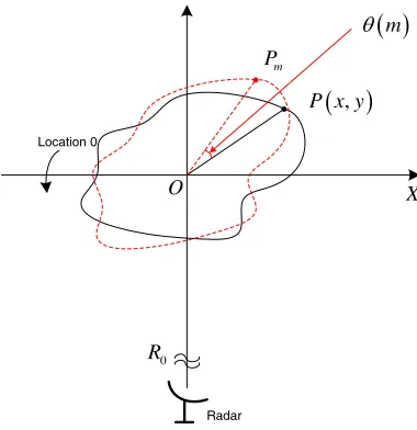
Figure 1 shows the geometry of ISAR imaging, where the translational motion of target has been
compensated, and the target can be viewed to be rotating around the center O. Linear frequency
modulated (LFM) signal, namely chirp signal, is one of the most used waveform in ISAR radar. Suppose the transmitted chirp signal is
sT (t) =rect
t Tp
exp
j2π
fct+ 1 2γt
2
(1)
where rect(u) =
1|u| ≤1/2
0|u|>1/2 . fc represents the center frequency,Tp the pulse width,γ the slope of the frequency modulation, and tthe fast time.
For the scattering point which locates at P(x, y) originally, after pulse compression by matched filtering, the echo of themth pulse reflected byP(x, y) can be written as:
sR(t, m) =psinc
Tpγ
t−2Rc(m)
exp
−j4πR(m)
λ
Location 0
)
,P x y
( )
mθ
X
0 R
Radar
O
m
P
(
Figure 1. Model of ISAR imaging.
wherep is the reflectivity coefficient of P(x, y) and λthe wavelength of signal. Let us define R(m) as the instantaneous range from P(x, y) to radar, and it can be denoted as
R(m) =R0+ycosθ(m) +xsinθ(m), (3)
whereθ(m) is the instantaneous rotation angle of themth pulse. And considering the angle is usually very small in ISAR, theR(m) can be approximated as
R(m)≈Ro+y+xθ(m) (4)
Andθ(m) can be approximated by Taylor expansion as
θ(m)≈ωtm+ 0.5αt2m+σt2m (5) wheretm is the slow time, andω andα are rotation velocity and acceleration, respectively. Therefore, the reflected signal can be approximated as
sR(t, m)≈psinc
Tpγ
t−2 (Ro+y) c
exp
−j4π
Ro+y+x
ωtm+ 0.5αt2m
λ
(6)
Suppose that there are K scatters in the mth range cell and the correspond range of which is
r(t) = 2 (Ro+ym)/c. The rotational motion is assumed to be stationary. After neglecting some constant term and high-order term, the signal ofmth range cell can be denoted as
sR(m)≈ K
k=1
pkexp
−j2π
2xkω
λ
m
(7)
where pk denotes thekth scattering point’s intensity. Let fk = 2xkωλ denote the Doppler frequency of the kth scatter. The cross-range compression is achieved by applying Fourier transform in each range cell. For themth range cell, we can get the compression result as
sR(fd) = K
k=1
pkδ(fd−fk) (8)
Considering the sampling window in the cross-range domain, the δ(·) function will be substituted by
sinc(·).
We build a dictionary Ψ, and the ith element of Ψ is ψi = exp [−j2πfd(i)m]. Let matrix SR denote the coherent integrated echoes for one image, where each row of SR is one profile of target and all the profiles are aligned by every range bin. The measurement ofSR can be presented as
where n is the measuring noise and P the 2D ISAR image of target, which denotes the scatters distribution in range and cross-range dimensions. Therefore, the ISAR imaging can be viewed as the inverse problem of (9). In conventional RD imaging, the sampling in cross-range dimension is uniform according to the Nyquist theory. The number of echoes is adequate for the Doppler analysis in cross-range dimension, which means the matrix Ψ in (9) is full rank and invertible. Assuming the measuring errors can be ignored or compensated, the RD imaging algorithm can be denoted simplified as
P=ΨSR (10)
where Ψ is the inverse of matrix Ψ. In RD imaging, applying Fourier transform in azimuth direction is the method of cross-range focal. So, the matrix Ψ in (10) is the inverse Fourier matrix.
2.2. Compensation of Phase Errors in ISAR Imaging
The model in (10) is the idealized model without errors, which is impossible in practical applications. Because only rotational motion of target contributes to the Doppler spectrum in ISAR imaging, the translational motion is undesirable and needs to be eliminated before applying cross-range focusing. Theoretically, it can be compensated based on the measured parameters of motion, such
as speed and trajectory of target [17]. However, due to the uncooperative motion of target and
the imprecision of radar system, there are always errors in the measurements. So, more accurately estimation and compensation is needed. The compensation of motion error usually consists of range alignment and phase compensation. Range alignment is relatively easier to realize based on maximum autocorrelation [18] or minimum-entropy of profiles [19]. Suppose the envelop of profiles are aligned and we focus on the phase error of ISAR observation in this paper.
Phase error is usually different for different echoes, and the influence of phase errors in the measurement can be expressed as
Y=ESR=EΨP. (11)
where E is a diagonal matrix diag{e1,e2· · ·eM}, and em = exp (jαm) is the phase error for the mth range profile.
In conventional ISAR imaging, there have been a lot of methods available to estimate the phase errors and compensate them. MEM algorithm attempts to estimate the phase errors by minimizing the image entropy with respect to em fori= 1,2,3,· · · , M and is proved to be effective [8]. To reduce the enormous amount of computation when applying MEM, an algorithm of fast minimum entropy phase compensation (FMEPC) was proposed in [20], which has both good autofocusing effect and computation efficiency. The advantages of FMEPC algorithm have been demonstrated by processing all kinds of ISAR imaging and is one of the most used algorithm in practical applications.
3. COMPENSATION OF PHASE ERROR WITH LIMITED PULSES IN CS ISAR IMAGING
3.1. CS ISAR Imaging
In the aforementioned section, the models of RD ISAR measuring process and conventional phase compensation have been built. In most cases of ISAR, there are only a few strong scattering points in one range bin, and the count of scattering centers is much smaller than measurements. As depicted in (10), the matrix of image P is sparse, and every column of P is also sparse. So, we can say that the echoes of target is compressive in the cross-range dimension, and Ψ is the sparse dictionary.
The theory of CS suggests that the compressive measurement can be applied and the signal can be reconstructed, as long as the signal is sparse itself or compressive in some dictionary, and the measurement matrix satisfies the restricted isometry property condition. Based on this, CS ISAR imaging has been a hot spot of research in recent years. It has been proposed in [21] that ISAR image can be reconstructed using much fewer pulses than needed by RD algorithm, and the pulses are sampled with random pulse repetition interval (PRI). Let Y denote the measurement of limited pulses and the observation can be viewed as selecting a few echoes from uniform sampled echoes SR, which can be denoted as
The dimension of measuring matrix Φ isL×M and L < M, where M is the number of whole pulses in uniform observation. Φcan be obtained by selecting someLrows fromM×M identical matrixIM.
And the image can be reconstructed by solving the problem as
P= arg min
P {λY−ΦΨP2+βP1} (13)
whereλandβ are the regularization parameters, which specify the strengths of the contribution of the reconstruction error and target regularization term, respectively.
As we can see, this model only takes into account the additive noise in measurement, and it assumes the range profiles are aligned perfectly and the target is consistent with the model of rotational platform in Fig. 1. Unfortunately, this assumption is way too idealized, while most of the real ISAR radars can’t satisfy this requirement. The phase errors in real data are so serious that sometimes we can’t even obtain any focused image without compensation.
A simple simulation is provided to prove the importance of phase compensation in CS ISAR
imaging. The scattering point model of target is given in Fig. 2(a), and the pulses of radar are
transmitted randomly with only 50% of the PRF in RD imaging. The number of pulses is inadequate for RD imaging, thus CS algorithm is utilized to reconstruct the image of target from limited echoes.
Firstly, no phase noise is added in echoes and the the CS imaging algorithm in [21] is applied to reconstruct the image of target. The result is shown in Fig. 2(a). The CS reconstruction can obtain focused image using much fewer pulses. Secondly, some random phase noises are added in the simulated echoes and the image is reconstructed using the same method. As shown in Fig. 2(b), the image is contaminate seriously by the phase errors.
Moreover, we try to compensate the phase error using conventional method. We choose FMEPC method, which is one of the most common and effective algorithm in RD imaging, to deal with the phase errors in inadequate pulses. However, as shown in Fig. 2(c), the effect of compensation is quite poor and the shadowing in cross-range is still very serious. It proves that the FMEPC is not working well in these pulses with non-uniform PRI.
The non-uniform PRI and inadequate pulses are the main reason why conventional method fails in CS ISAR imaging. In the processing of FMEPC, Fourier transform is very important to generate ISAR image in every iteration. However, the Fourier transform is invalid when pulses are inadequate and non-uniformly sampled. Actually, this is also the main reason why other conventional phase compensating algorithms fail in CS ISAR imaging. The phase compensating method has to be proposed considering the particularity of CS measurement, which is the aim of this paper.
Cross range (m)
Range (m)
-30 -20 -10 0 10 20 30 -30
-20
-10
0
10
20
30-Cross range (m)
Range (m)
-30 -20 -10 0 10 20 30 -20
-10
0
10
20
Cross range (m)
Range (m)
-30 -20 -10 0 10 20 30 -20
-10
0
10
20
Cross range (m)
Range (m)
-30 -20 -10 0 10 20 30 - 20
-10
0
10
20
(a) (b) (c) (d)
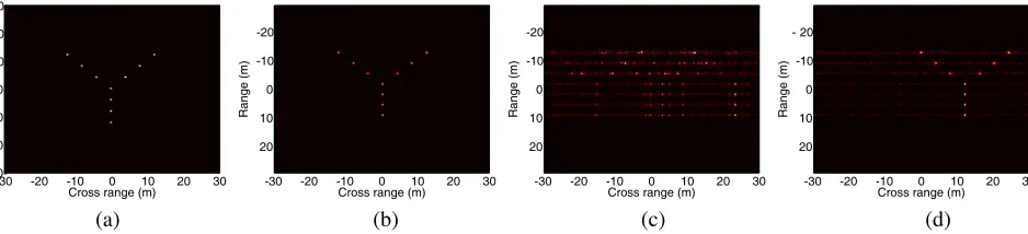
Figure 2. CS reconstructed image of a simulated target using random selecting pulses with phase
errors. (a) The model of target. (b) The reconstructed result when there is no phase errors in the echoes. (c) Phase error is added and the image is reconstructed without any phase compensation. (d) The phase error is compensated using conventional FMEPC algorithm before CS reconstruction.
3.2. Compensation of Phase Error in CS ISAR
we change the observation model (12) to
Y=ΦESR=ΦEΨP+n. (14)
whereE is a diagonal matrix and the diagonal elements are unknown phase errors. To reconstruct the image P, we need to estimate the phase errors at compensate them. So, we pose the problem of joint target reconstruction and phase error estimation as the minimum cost solution of the following cost function
T(P,E) =λY−ΦEΨP2+βP1+ηE(P) (15) where whereλ,β andηare regularization parameters, andE(P) is the entropy of reconstructed image.
E(P) can be obtained as
E(P) =− N
n=1
M
m=1
(D(n, m) ln (D(n, m))) (16)
where theD(n, m) denotes the density of scattering intensity and is calculated as
D(n, m) = P(n, m)
2
N
n=1
M
m=1
P(n, m)2
(17)
Both the image and the phase errors can be obtained by solving (15). To solve this problem, we propose an iterative algorithm, which cycles the steps of image reconstruction and phase error estimation. First, we assume a set of initialized phase errors, and the cost function is changed into the same with conventional CS ISAR problem as (13). After solving that, an image is reconstructed, and we turn to evaluate the phase errors by minimizing the entropy of image. Before next iteration, the measuring matrix is updated using the newly estimated phase errors. The flow of our algorithm is outlined as follows:
Step 1: Initialize the iterative counter asl= 1, the vector of phase errorel=0, and Pl =P; Step 2: Update the measuring matrix as Ml = ΦElΨ, where El = diag (exp (−jel)), and reconstruct the image by solving Pl+1= arg min
P {λY−MlP2+βP1};
Step 3: Ifl > 1, calculate δ =Pl+1−Pl22
Pl22, and terminate the iteration if δ is less than preset threshold, else continue;
Step 4: Estimate the phase errors by solving el+1 = arg min
e {E(Pl+1)};
Step 5: Letl=l+ 1 and return to step 2.
In the iteration, the steps 2 and 3 are the key steps. For Step 2, it can be seen as an standard form of CS ISAR imaging problem, which can be solved by existing CS methods, such as orthogonal matching pursuit (OMP) [22], basis pursuit (BP) [23], and smoothed0 (SL0) [24]. Among those methods, BP is
usually more stable but computational complex. SL0 has been proved to have a good trade-off between accuracy and complexity, and does not need prior knowledge about sparsity level of original signal [25]. We choose SL0 to reconstruct the image of target in our algorithm.
For Step 3, we use the the similar method as FMEPC to estimate the phase errors in pulses. The phase error of the mth echo can be estimated as
exp (je(m)) = ω
∗(m)
ω(m)2 (18)
And
ω(m) = N
n=1
S(n, m) L
q=1
ln (P(n, q)2)P∗(n, q) exp
−j2π(k−L1) (q−1)
(19)
where S is the range profiles after range alignment, L is the number of pulses and N is the number of range bins in one pulse.
preset. The iterative structure of our proposed method is similar with the algorithm proposed in [26, 27], the convergence of such iteration has been proved in [26, 27]. So the convergence of this algorithm is guaranteed and will be proven in the following experiments.
3.3. Fast Compensation by Extracting Target Area
As we know, the reconstruction of image in Step 2 of our algorithm is the most complex processing. The computational complexity of CS reconstruction has always been the bottle-neck of CS application, because it has a lot of matrix multiplication to process, which is very time-consuming. Reducing the dimension of matrix is the best and direct method to reduce the computation complexity.
In CS ISAR imaging, the dimension of measuring matrix isL×N, whereLis the count of selected pulses andN is the number of range bins in one pulse. As we know, the target usually occupies only a few range bins and the other bins are only noise. When doing phase compensation, the range bins with target scatters contribute much more than others with noise. So, we propose to extract the target area before compensating the phase errors. The aim of target extraction is selecting some range bins with strong scattering intensity and forming a smaller profile image to represent the whole image. And then the phase compensation can be done using the extracted profiles.
To extract the target range bins more accurately, we use the average range bins to determine the threshold of extraction. After alignment of range envelop, we calculate the average range profile using non-coherent accumulation. Assume the noise in complex profiles is Gauss-distributing with the standard deviation of σ, thus the amplitude distribution of noisy range bins is Rayleigh distribution.
The standard deviation of noise σ can be determined from the measurements without target and can
be treated as prior information in the extraction. According to the probability distribution of Rayleigh distribution, the threshold of amplitude can be obtained as
κ=
−2σ2ln (P
f) (20)
wherePf is the false-alarm probability.
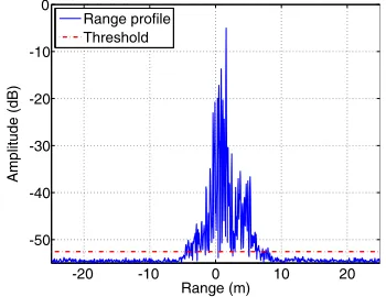
It is easy to calculate the threshold κwhen we determine a demanded false-alarm probability. We choose Pf = 95% as the default probability, and it is proved to be able to extract most of the range bins with scattering points in most cases. We use the algorithm in real radar data and the result is shown in Fig. 3. The range profile in this figure is the average range profile of an flying aircraft, which is sampled by an experimental radar. The threshold determined by (20) can help us extract the range bins with scattering points.
-20 -10 0 10 20 -50
-40 -30 -20 -10 0
Range (m)
Amplitude (dB)
Range profile Threshold
Figure 3. Extract range bins with target scattering points from the whole range profile.
By extraction, the range bins with higher average amplitude are kept and others are discarded
temporarily. The extracted profiles form a new smaller matrix SR and is processed by our proposed
As can be seen, the extraction can reduce the size of measurements sharply. In Fig. 3, the length of original range profile is 1000 bins, and it reduces to 215 after extraction. The reduction of matrix size makes the computation of CS reconstruct really faster, which is very convenient for iteration processing. We will demonstrate it in the following experiments.
4. SIMULATION AND EXPERIMENT RESULTS
In this section, the proposed method is applied in a number of scenarios with both simulated data and experimental data. The results are presented to show the effectiveness of the proposed method.
4.1. Simulation Resutls
Table 1. Parameters for the imaging radar in simulation.
Center frequency 10 GHz
Bandwidth 300 MHz
Pulse duration 50µs
Chirp rate 6×10¹²Hz/s
Number of range bins 384
Number of pulses in CPI 256
Pulse repeat frequency 1000 Hz
To evaluate the performance of proposed method, the echo data of a LFM radar is generated with parameters given in Table 1. The model of scattering points for simulated target is presented in Fig. 4. To simulate the compressive measurement with limited pulses, we randomly select part of echoes from the M = 256 original pulses with nonuniform PRIs. The number of selected pulses are set to be
L=M×δ, where δ <1 is the compressed ratio.
Cross range (m)
Range (m)
-30 -20 -10 0 10 20 30 -30
-20
-10
0
10
20
30
Figure 4. The reflectivity distribution of simulated target.
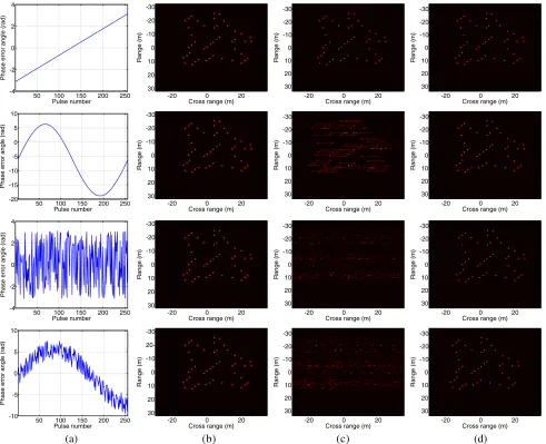
First, we do some simulations to test the feasibility of our proposed algorithm. We divide the phase errors of echoes into four types, namely low-order, high-order, random and combined errors. The combined error consists of the other three types and is more consistent with the actual radar applications. Four types of phase error are all tested in our simulations, and the reconstructed images are shown in Fig. 5 respectively. The compressed ratios in four figures are all set to be 50%.
50 100 150 200 250 -4 -2 0 2 4 Pulse number
Phase error angle (rad)
Cross range (m)
Range (m)
-20 0 20
-30 -20 -10 0 10 20 30
Cross range (m)
Range (m)
-20 0 20
-30 -20 -10 0 10 20 30
Cross range (m)
Range (m)
-20 0 20
-30 -20 -10 0 10 20 30
50 100 150 200 250 -20 -15 -10 -5 0 5 10 Pulse number
Phase error angle (rad)
Cross range (m)
Range (m)
-20 0 20
-30 -20 -10 0 10 20 30
Cross range (m)
Range (m)
-20 0 20
-30 -20 -10 0 10 20 30
Cross range (m)
Range (m)
-20 0 20
-30 -20 -10 0 10 20 30
50 100 150 200 250 -4 -2 0 2 4 Pulse number
Phase error angle (rad)
Cross range (m)
Range (m)
-20 0 20
-30 -20 -10 0 10 20 30
Cross range (m)
Range (m)
-20 0 20
-30 -20 -10 0 10 20 30
Cross range (m)
Range (m)
-20 0 20
-30 -20 -10 0 10 20 30
50 100 150 200 250 -10 -5 0 5 10 Pulse number
Phase error angle (rad)
Cross range (m)
Range (m)
-20 0 20
-30 -10 0 10 20 30
Cross range (m)
Range (m)
-20 0 20
-30 -20 -10 0 10 20 30
Cross range (m)
Range (m)
-20 0 20
-30 -20 -10 0 10 20 30
(a) (b) (c) (d)
Figure 5. Imaging results under different types of phase errors. The phase errors in four rows are
lower-order errors, high-order errors, random errors and combined errors, respectively. The figures in column (a) are the plotted phase errors in pulses; (b) are the imaging results of RD algorithm using whole pulses; (c) are CS reconstructed images with 50% pulses without compensation of phase errors; (d) are images reconstructed with 50% pulses and the phase errors are compensated using proposed algorithm.
fails to obtain focused image under the last three types of phase errors. It is shown that the proposed algorithm in this paper performs well in all types of phase errors, which improves the imaging quality remarkably. Because the combined error is the most common in practical applications, only this kind of error is taken into account in the following simulations.
Cross range (m)
Range (m)
-20 0 20
-30
-20
-10
0
10
20
30
Cross range (m)
Range (m)
-20 0 20
-30
-20
-10
0
10
20
30
Cross range (m)
Range (m)
-20 0 20
-30
-20
-10
0
10
20
30
(a) (b) (c)
Cross range (m)
Range (m)
-20 0 20
-30
-20
-10
0
10
20
30
Cross range (m)
Range (m)
-20 0 20
-30
-20
-10
0
10
20
30
Cross range (m)
Range (m)
-20 0 20
-30
-20
-10
0
10
20
30
(d) (e) (f)
Figure 6. The setting of simulated data and results of reconstruction using proposed algorithm. (a)–(c)
are reconstructed images when no target extraction is done before iterations, and the compressed ratios of random pulse-selection are 75%, 50% and 25%, respectively. (d)–(f) are reconstructed images using proposed target extracting method before iterations, with the compressed ratios 75%, 50% and 25%, respectively.
Then, the extraction of target is carried out before reconstructing iterations. The reconstructed images under different compressed ratios are shown in Figs. 6(d)–(f), and other results such as running time are also presented in Table 2.
Table 2. Comparison of reconstructing results using simulated data.
Using extraction Without extraction
Compressed ratio 75% 50% 25% 75% 50% 25%
Average image entropy 5.526 5.955 6.289 5.508 5.963 6.255
Average running time 25.510 s 20.220 s 7.969 s 123.235 s 85.435 s 32.501 s
Average iterations 9.4 9.8 9.4 11.4 10.2 10
The results of simulation prove that our iterative algorithm performs stably well in different compressed ratios. As the compressed ratio becomes smaller, the quality of reconstruction is reduced, while the computational cost reduces. This is an inherent problem of CS, and best tradeoff between quality and computation cost must be made by selecting the compressed ratio according to the actual need. Imaging quality has to be sacrificed relatively to obtain faster reconstruction, and vice versa.
4.2. Experiment Results
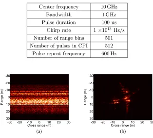
The proposed imaging method is also tested using real radar data. In this experiment, the echo data is generated by an real experimental LFM ISAR imaging radar, the parameters of which is presented in Table 3. LFM waveform is used by the radar. The target is a flying civilian aircraft and distance is about 10 km. The fully sampled data is acquired using an experimental digital receiver, which is still in progress of building and testing. Due to the imperfection of radar system, the signal to noise ratio of echo data is not quite high and the phase errors of echo data are so serious that no focal image can be obtained without effective phase compensation. The RD imaging result without phase compensation is shown in Fig. 7(a). This is quite an appropriate opportunity to test our compensating method in practical application. After compensating the phase errors using FMEPC algorithm, a well-focused image can be obtained, as is shown in Fig. 7(b).
Table 3. Parameters for the real experimental radar.
Center frequency 10 GHz
Bandwidth 1 GHz
Pulse duration 100 us
Chirp rate 1 ×10¹³ Hz/s
Number of range bins 501
Number of pulses in CPI 512
Pulse repeat frequency 600 Hz
Cross range (m)
Range (m)
-30 -20 -10 0 10 20 30 -30
-20
-10
0
10
20
30
Cross range (m)
Range (m)
-30 -20 -10 0 10 20 30 -30
-20
-10
0
10
20
30
(a) (b)
Figure 7. Imaging result of aircraft using full original data and range-Doppler imaging method. (a) The
image is obtained without any compensation of phase errors. (b) MEM method is used to compensate the phase errors of pulses.
Then we apply random pulse selection by setting the compressed ratio to be Δs = 75%, 50% and 25%, respectively. Fig. 8 shows the reconstructed images using our method. It can be seen that the image is well focused. The focusing quality reduces slightly as the compressed ratio becomes smaller, which is consistent with the results of simulation in Section 4.1. When the ratio is 25%, there appears obvious noise and some defocusing effect in the reconstructed image, but the outline of aircraft still can be recognized. In this experiment, the number of pulses and the number of range bins are both relatively larger than simulation, so the computational time is longer. When compressed ratio is 50%, the average running time of the proposed iterative algorithm is 283.060 s and the average number of iterations is 27.5.
Cross range (m)
Range (m)
-20 -10 0 10 20 -30 -20 -10 0 10 20 30
Cross range (m)
Range (m)
-20 -10 0 10 20 -30 -20 -10 0 10 20 30
Cross range (m)
Range (m)
-20 -10 0 10 20 -30 -20 -10 0 10 20 30
(a) (b) (c)
Cross range (m)
Range (m)
-20 -10 0 10 20 -30 -20 -10 0 10 20 30
Cross range (m)
Range (m)
-20 -10 0 10 20 -30 -20 -10 0 10 20 30
Cross range (m)
Range (m)
-20 -10 0 10 20 -30 -20 -10 0 10 20 30
(d) (e) (f)
Figure 8. The reconstructed images using proposed reconstructing and phase compensating method.
(a)–(c) are reconstructed images when no target extraction is done before iterations, and the compressed ratios of random pulse-selection are 75%, 50% and 25%, respectively. (d)–(f) are reconstructed images using proposed target extracting method before iterations, and the compressed ratios is the same with those above.
Cross range (m)
Range (m)
-20 -10 0 10 20 -30 -20 -10 0 10 20 30
Cross range (m)
Range (m)
-20 -10 0 10 20 -30 -20 -10 0 10 20 30
Cross range (m)
Range (m)
-20 -10 0 10 20 -30 -20 -10 0 10 20 30
(a) (b) (c)
Figure 9. The imaging results which are obtained after phase compensation using conventional
FMEPC algorithm. In (a)–(c) the compressed ratios of random pulse-selection are 75%, 50% and 25%, respectively.
5. CONCLUSION
This paper has proposed a method to compensate the phase errors in CS ISAR imaging with limited pulses. The proposed method can jointly reconstruct the images and estimate the phase errors using an iterative algorithm. The steps of target reconstruction and phase error estimation are cycled in the iteration, and the reconstructed quality improved as the phase errors are compensated step by step. In the step of target reconstruction, a standard CS reconstruction algorithm is implemented using SL0 algorithm. In the step of phase error estimation, a minimum entropy optimization algorithm is used. A method of target extraction from range profiles is also introduced, where the dimension of measured matrix can be reduced sharply. The computation load of CS reconstruction of image during the iteration is reduced obviously after the extraction is done in advance. Both simulation and experiment results from ISAR radar have been presented to show the effectiveness of the proposed method.
ACKNOWLEDGMENT
This work was supported by the National Natural Science Foundation of China (No. 61471373). The authors would like to thank the editors and the anonymous reviewers for their helpful comments to improve the paper quality.
REFERENCES
1. Ozdemir, C., Inverse Synthetic Aperture Radar Imaging With MATLAB Algorithms, John Wiley
and Sons, INC., Hoboken, New Jersey, 2012.
2. Zhou, F., X. Bai, M. Xing, and Z. Bao, “Analysis of wide-angle radar imaging,”IET Radar, Sonar and Navigation, Vol. 5, No. 4, 449–457, 2011.
3. Liu, Y., J. Zou, S. Xu, and Z. Chen, “Nonparametric rotational motion compensation technique for high-resolution isar imaging via golden section search,”Progress In Electromagnetics Research M, Vol. 36, 67–76, 2014.
4. Chen, C.-C. and H. C. Andrews, “Target-motion-induced radar imaging,” IEEE Transactions on
Aerospace and Electronic Systems, Vol. 16, No. 1, 2–14, 1980.
5. Wahl, D. E., P. H. Eichel, D. C. Ghiglia, and C. V. Jakowatz, Jr., “Phase gradient autofocusa robust tool for high resolution sar phase correction,” IEEE Transactions on Aerospace and Electronic Systems, Vol. 30, No. 3, 827–835, 1994.
6. Martorella, M., F. Berizzi, and B. Haywood, “Contrast maximisation based technique for 2-d isar autofocusing,”Sonar and Navigation IEE Proceedings-Radar, Vol. 152, No. 4, 253–262, 2005. 7. Berizzi, F., M. Martorella, A. Cacciamano, and A. Capria, “A contrast-based algorithm for
synthetic range-profile motion compensation,” IEEE Transactions on Geoscience and Remote
Sensing, Vol. 46, No. 10, 3053–3062, 2008.
8. Xi, L., L. Guosui, and J. Ni, “Autofocusing of isar images based on entropy minimization,” IEEE Transactions on Aerospace and Electronic Systems, Vol. 35, No. 4, 1240–1252, 1999.
9. Donoho, D. L., “Compressed sensing,” IEEE Transactions on Information Theory, Vol. 52, No. 4, 1289–1306, 2006.
10. Cand Es, E. J., J. Romberg, and T. Tao, “Robust uncertainty principles: Exact signal
reconstruction from highly incomplete frequency information,”IEEE Transactions on Information Theory, Vol. 52, 489–509, 2006.
11. Herman, M. A. and T. Strohmer, “High-resolution radar via compressed sensing,” IEEE
Transactions on Signal Processing, Vol. 57, 2275–2284, 2009.
12. Ender, J., “On compressive sensing applied to radar,”Signal Processing, Vol. 90, 1402–1414, 2010.
13. Amin, M. G. and F. Ahmad, “Compressive sensing for through-the-wall radar imaging,” Journal
of Electronic Imaging, Vol. 22, 030901, 2013.
15. Daiyin, Z., Y. Xiang, and Z. Zhaoda, “Algorithms for compressed isar autofocusing,” IEEE CIE International Conference on Radar, 533–536, IEEE, Chengdu, 2011.
16. Zhu, D., Y. Li, X. Yu, W. Zhang, and Z. Zhu, “Compressed isar autofocusing: Experimental
results,” 2012 IEEE Radar Conference (RADAR), 425–430, 2012.
17. Lin, Q., Z. Chen, Y. Zhang, and J. Lin, “Coherent phase compensation method based on direct if sampling in wideband radar,”Progress In Electromagnetics Research, Vol. 136, 753–764, 2013. 18. Wang, J. and X. Liu, “Improved global range alignment for isar,”IEEE Transactions on Aerospace
and Electronic Systems, Vol. 43, No. 3, 1070–1075, 2007.
19. Zhu, D., L. Wang, Y. Yu, Q. Tao, and Z. Zhu, “Robust isar range alignment via minimizing the entropy of the average range profile,”IEEE Geoscience and Remote Sensing Letters, Vol. 6, No. 2, 204–208, 2009.
20. Xiaohui, Q., H. W. C. Alice, and Y. S. Yam, “Fast minimum entpy phase compensation for isar imaging,”Journal of Electronics and Information Technology, Vol. 26, No. 10, 1656–1661, 2004. 21. Zhang, L., M. Xing, C.-W. Qiu, J. Li, and Z. Bao, “Achieving higher resolution isar imaging with
limited pulses via compressed sampling,” IEEE Geoscience and Remote Sensing Letters, Vol. 6, 567–571, 2009.
22. Tropp, J. A. and A. C. Gilbert, “Signal recovery from random measurements via orthogonal matching pursuit,” IEEE Transactions on Information Theory, Vol. 53, 2007.
23. Chen, S. S., D. L. Donoho, and M. A. Saunders, “Key words. overcomplete signal representation, denoising, time-frequency analysis, time-scale,” Society for Industrial and Applied Mathematics, Vol. 20, No. 1, 33–61, 1998.
24. Mohimani, G. H., M. Babaie-Zadeh, and C. Jutten, “A fast approach for overcomplete sparse
decomposition based on smoothed l0 norm,” IEEE Transactions on Signal Processing, Vol. 57,
289–301, 2007.
25. Liu, J., S. Xu, X. Gao, and X. Li, “Compressive radar imaging methods based on fast smoothed l0 algorithm,” 2012 International Workshop on Information and Electronics Engineering, Vol. 29, 2209–2213, Elsevier Ltd., 2012.
26. Samadi, S., M. C¸ etin, and M. A. Masnadi-Shirazi, “Sparse representation-based synthetic aperture radar imaging,”IET Radar, Sonar & Navigation, Vol. 5, No. 2, 182–193, 2011.
27. Yang, J., X. Huang, J. Thompson, T. Jin, and Z. Zhou, “Compressed sensing radar imaging
with compensation of observation position error,” IEEE Transactions on Geoscience and Remote