[NORMAL] Improvement of Computational Performance of Implicit Finite Difference Time Domain Method

(1)

Improvement of Computational Performance of Implicit Finite

Diﬀerence Time Domain Method

Hasan K. Rouf*

Abstract—Diﬀerent solution techniques, computational aspects and the ways to improve the

performance of 3D frequency dependent Crank Nicolson finite difference time domain (FD-CN-FDTD) method are extensively studied here. FD-CN-FDTD is an implicit unconditionally stable method allowing time discretization beyond the Courant-Friedrichs-Lewy (CFL) limit. For the solution of the method both direct and iterative solver approaches have been studied in detail in terms of computational time, memory requirements and the number of iteration requirements for convergence with different CFL numbers (CFLN). It is found that at higher CFLN more iterations are required to converge resulting in increased number of matrix-vector multiplications. Since matrix-vector multiplications account for the most significant part of the computations their efficient implementation has been studied in order to improve the overall efficiency. Also the scheme has been parallelized in shared memory architecture using OpenMP and the resulted improvement of performance at different CFLN is presented. It is found that better speed-up due to parallelization always comes at higherCFLN implying that the use of FD-CN-FDTD method is more appropriate while parallelized.

1. INTRODUCTION

In the finite difference time domain (FDTD) method, the size of time discretization is limited by the smallest spatial step due to the CFL stability condition [1]. To overcome this drawback of explicit FDTD method recently researchers have focused on developing alternative unconditionally stable schemes which can overcome the upper bound on the time discretization and thereby reduce the total simulation time. Crank Nicolson FDTD (CN–FDTD) [2] is an unconditionally stable method and in this work we deal with the frequency dependent version of it (FD-CN-FDTD method) [3, 4]. Since Crank Nicolson based schemes require the solution of computationally expensive large sparse matrices, extensive studies on different computational aspects are essential to make them a promising affordable alternative to the explicit FDTD method.

In this paper we studied different computational aspects of 3D frequency dependent CN–FDTD (FD-CN-FDTD) method [3]. For the solution of the method both direct and iterative solver approaches have been studied in detail in terms of computational time and memory requirements. Furthermore, two best-known iterative methods, Bi-Conjugate Gradient Stabilised (BiCGStab) and Generalised Minimal Residual (GMRES), were compared in terms of the number of iteration requirements for convergence with different CFLN, CPU-time and memory requirements. Here CFLN ≡ Δt/Δt_CFL with Δt being the time discretization used in the simulation and Δt_CFL denoting the maximum time discretization allowed by the CFL stability condition. As in each time step of the FD-CN-FDTD method, matrix-vector multiplication needs to be performed a number of times, it has a significant contribution in the overall computational performance. This is because matrix-vector multiplications are performed

Received 24 May 2015, Accepted 1 July 2015, Scheduled 8 July 2015 * Corresponding author: Hasan Khaled Rouf (hasan [email protected]).

(2)

repeatedly until the solution converges. Also it is found that more iterations are required to converge at higher CFLN resulting in increased number of matrix-vector multiplications. Therefore, eﬃcient implementation of matrix-vector multiplications have been studied. We also performed parallelization by using OpenMP in a shared memory architecture and studied the resulted speed-up of performance at diﬀerent CFLN. The resulted operations from the increased number of iteration to converge at higher CFLN are more suitable for parallelization. Therefore, better speed-up by parallelization is seen at higherCFLN which indicates that the use of FD-CN-FDTD method is more appropriate while parallelized.

The paper is organized as follows: Section 2 brieﬂy describes the FD-CN-FDTD method. Performance of Gaussian elimination based direct methods is presented in Section 3 while Section 4 presents that of iterative methods. How the computational eﬃciency of FD-CN-FDTD method can be further improved is discussed in Section 5.

2. FREQUENCY DEPENDENT CN-FDTD METHOD

In FD-CN-FDTD scheme [3] frequency dependence of single-pole Debye media has been incorporated by auxiliary diﬀerential equation method [5]. In material independent form, Maxwell’s curl equations are:

∇ ×E=−∂B

∂t and∇ ×H= ∂D

∂t , where E,H,D and B are the electric field, magnetic field, electric flux density and magnetic flux density, respectively. In frequency domain, the constitutive relationships for isotropic, linear, non-magnetic, single-pole Debye electrically-dispersive media are: B = μ0H and

D=0(∞+

S−∞

1 +jωτD−j

σ ω0

)E, where0 andμ0 are the free-space permittivity and permeability, and

Sis the static permittivity,∞the optical permittivity,τDthe relaxation time,σthe static conductivity

and ω the angular frequency. The previous equation can be re-written as

(jω)2τDD+jωD= (jω)20∞τDE+jω(0S+στD)E+σE (1)

Mapping frequency domain (jω)minto time domain _∂t∂mm Eq. (1) can be written as a diﬀerential equation

in time domain:

τD∂ 2_D

∂t2 +

∂D

∂t =0∞τD∂ 2_E

∂t2 + (0S+στD)

∂E

∂t +σE (2)

Crank-Nicolson method [6] is applied to Maxwell’s curl equations, the constitutive relationships and Eq. (2). Algebraic manipulation of the resultant equations yields an equation with only electric ﬁeldEn+1 terms:

Exn+1−ξ_ξ1 4 Δt 2 2 ₁ μ ∂2_E

xn+1

∂y2 +

ξ1 ξ4 Δt 2 2 ₁ μ ∂2_E

yn+1

∂x∂y + ξ1 ξ4 Δt 2 2 ₁ μ ∂2_E

zn+1

∂z∂x − ξ1 ξ4 Δt 2 2 ₁ μ ∂2_E

xn+1

∂z2

=ξ1 ξ4

Dxn+ξ1 ξ4

Δt 2

∂Hzn

∂y + ξ1 ξ4 Δt 2 2 1 μ

∂2_E xn

∂y2 −

ξ1 ξ4 Δt 2 2 1 μ

∂2_E yn ∂x∂y − ξ1 ξ4 Δt 2

∂Hyn

∂z − ξ1 ξ4 Δt 2 2 1 μ

∂2_E zn

∂z∂x

+ξ1 ξ4 Δt 2 2 1 μ

∂2_E xn

∂z2 +

ξ1 ξ4 Δt 2 2_∂H zn ∂y − ξ1 ξ4 Δt 2 2 _∂H yn ∂z + ξ2

ξ4Dx n₊ξ3

ξ4Dx

n−1₋ξ5

ξ4Ex n₋ξ6

ξ4Ex

n−1 ₍₃₎

Here ξ1, ξ2, ξ3, ξ4, ξ5, ξ6 are space dependent and functions of the Debye parameters and time

discretization Δt as defined in [3]. Cyclic permutation of x, y and z in Eq. (3) yields the remaining two E-field equations. By applying them to each grid position in the computational space a system of linear equations ofAu=c is set up. Ais very large and highly sparse coefficient matrix,urepresents a vector with the electric field components to be solved, andcis the excitation vector. When the problem space is homogeneous,A is symmetric and otherwise asymmetric. The system of equations Au=c is solved to find theE field. ThenD and Hfields are calculated in an explicit manner from theE field.

3. SOLUTION BY DIRECT METHODS

(3)

Initialization

Form the sparse matrix & do LU decomposition

t= 0

Update [c] and use the same LU factors at each iteration to solve for E by forward/ backward substitution

H field Calculation

D field Calculation

t<t ?

Yes

End simulation No

t=t+1

Initialization

Form the sparse matrix

t=0

Update [c] and solve the

sparse matrix system Au=c by an iterative method to get E

H field Calculation

D field Calculation

Yes

End simulation No

t=t+1

Direct Solver Approach: Iterative Solver Approach:

max t<t ?max

Figure 1. Flowchart of the FD-CN-FDTD

method.

Figure 2. Observations from explicit FDTD and

FD-CN-FDTD schemes.

algorithm, a new vectorcis calculated for the right hand side, whileAis ﬁxed. Direct solvers factorizes

A (which dominates the computational time) only once before the beginning of the FDTD iteration. Once factorized, the same factors are repeatedly used at each time step to obtain u. For this reason, this method showed the potential to become more computationally eﬃcient than the iterative methods when a large number of FDTD iterations are needed, since at each time step only forward and backward solutions are required.

Numerical tests were performed with the direct solver using sparse Gaussian elimination in the FD-CN-FDTD method. A cubic computational region of size (30×30×30) cells was considered. Half of it was ﬁlled with medium 1 (S = 71.66, ∞= 34.58, σ = 0.49 S/m and τD= 5.65 ps) and the other

half with medium 2 (S = 87.34,∞= 49.13, σ= 0.69 S/m andτD= 26.89 ps). Az-directed dipole was

placed at (10, 15, 15) in medium 1, with a time evolution of a modulated Gaussian pulse centered at 3 GHz. Signals were recorded 10 cells away at (20, 15, 15) in medium 2. A uniform spatial sampling was taken (Δx= Δy = Δz= 10−3m). The first 600 time steps of theE_z field component at the observation point are shown in Figure 2 computed both with standard explicit frequency dependent (FD-)FDTD withCFLN = 1, and with FD-CN-FDTD withCFLN = 1, 3, 5. Good agreement between the signals from the unconditionally stable FD-CN-FDTD method beyond the CFL limit (CFLN >1) and explicit FD-FDTD was observed. For this numerical problem, CPU time required for LU decomposition was 633 minutes and average CPU time per iteration was 6.489 seconds when CFLN = 1 on dual AMD Opteron 280 with 8GB of memory. When the FDTD space was filled with homogeneous material of media 1 or when CFLN >1 there were no significant differences in these values.

Although direct solvers are robust and reliable, they are computationally more expensive than iterative solvers, unless parallelized, and require excessively large memory. For example, a 303 cells computational space (like the one described in the previous numerical test) solved by the direct solver in double precision using sparse Gaussian elimination requires 2.4 GB of memory whereas iterative solvers like BiCGStab and GMRES require only 62 MB and 65 MB, respectively. Thus for practical problems iterative solvers should be used.

4. SOLUTION BY ITERATIVE METHODS

(4)

Is the matrix Symmetric?

Is the matrix Symmetric positive-definite?

Are the extremal Eigenvalues Known? y CG n MinRES Or CG QMR CGS or BiCGStab Is the transpose

available? n

n

Is storage at a premium?

GMRES with long restart

Chebyshev or CG

MinRES: Minimal Residual method

CGS: Conjugate Gradient Squared method QMR: Quasi-Minimal Residual method CG: Conjugate Gradient method n

y y

n

y _y

Figure 3. Choosing an eﬀective iterative method.

Medium 2 Medium 1 x y z 15 80 80 80 Medium 4 Medium 3 Medium 5 20 24 91 2 Medium 2 Medium 1 Medium 4 Medium 3 Medium 5 s

Medium τ (ps) σ (S/m) 71.66 34.58 5.65 0.021

3.5

6.2 39.0 0.029 4.2

9.5 77.0 0.037 87.3449.1326.89 0.045

2.8 7.0 4.8 0.053

∋

8

∋

Figure 4. Computational environment for

numerical tests.

BiCGStab (inhomogeneous media) GMRES (inhomogeneous media) BiCGStab (homogeneous media) GMRES (homogeneous media)

Threshold of residual error

Number of iteration

100 200

10 -3

10 -6

10 -9

10 -12

50 150 250

Figure 5. Residual error versus number of

average iteration required by BiCGStab and GMRES for homogeneous and inhomogeneous cases (CFLN = 20).

0

CFLN

4 8 12 16 20

0

Average number of iteration

100 200

50 250

150

Figure 6. Average number of iterations required

for diﬀerent CFLN with residual error = 10−13_.

We compare the performances of BiCGStab and GMRES for two cases. The first one consists of an inhomogeneous medium, in a cubic space of size 803 cells, with 5 different media as shown in Figure 4. The second one involves the same cubic space of the previous case, now filled with a homogeneous medium with Debye parameters S = 6.2, ∞ = 3.5, σ = 0.029 S/m and τD = 39.0 ps. In both cases

a z-directed dipole hard source with a time variation given by a Gaussian pulse centered at 6.9 GHz, with 4.94 GHz bandwidth (−3 dB decay) was placed at the centre of the computational space. Spatial sampling was uniform: Δx = Δy = Δz = Δ = 10−3m. The time step is taken equal or above the CFL stability condition of the explicit FDTD. The level of accuracy in waveform compared with explicit frequency-dependent FDTD is the same as the one presented in Figure 2. Figure 5 shows the convergence pattern for CFLN = 20, plotting the residual error as a function of the average number of iterations required to achieve a speciﬁed accuracy. For example, to make the residual error lower than 10−8 _{BiCGStab requires about 45 iterations whereas GMRES requires about 97 iterations in both}

(5)

Figure 6 shows how the average number of iterations, required by BiCGStab and GMRES to converge, increases with the CFL number. Stopping criteria in this case was 10−13 _{and the reason for}

selecting this small value of convergence tolerance is, in FD-CN-FDTD, unlike frequency-independent CN-FDTD, D = E is used and therefore D can have a value of such small order because of (permitivitty). GMRES stagnates when convergence tolerance is below 10−13while BiCGStab can work even at a lower convergence tolerance. Both solvers require more iterations to converge as CFLN goes up but the rate of increase of iteration numbers with CFLN is higher for GMRES than for BiCGStab. Homogeneity does not aﬀect signiﬁcantly this rate, particularly, for BiCGStab. The change of iteration number withCFLN for convergence tolerance values from 10−12to 10−3 can be assumed from Figure 5. In FD-CN-FDTD, the total number of iterations required to complete the simulation decreases with

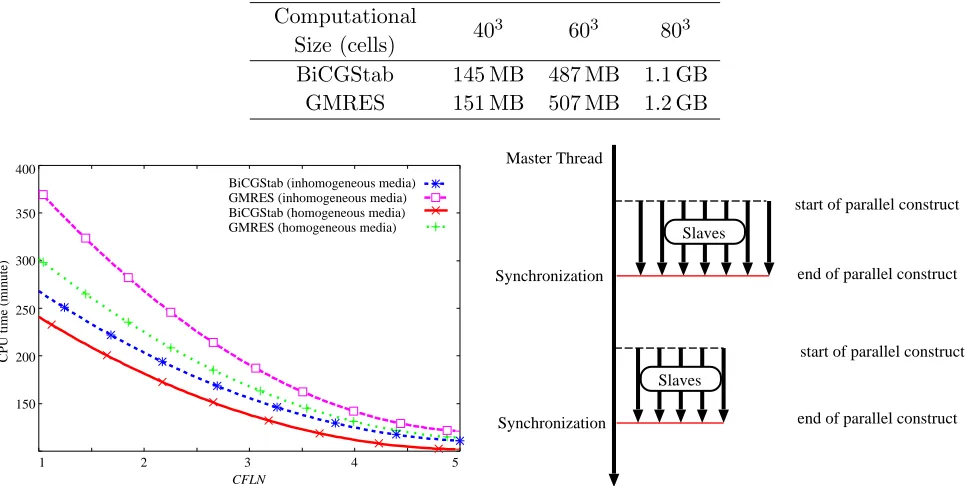
CFLN, but the increase of computational costs per iteration with CFLN, as shown in Figure 6, can undermine this positive effect unless the solution is very efficient. Figure 7 plots the CPU time required by BiCGStab and GMRES as a function ofCFLN. The case of stopping criterion of 10−13was employed and simulated to reach a fixed time instant by letting the code run for 1200/CFLN time steps on a dual AMD Opteron 280 with 8 GB of memory. Observe that the CPU-time decreases with CFLN, for both solvers, although GMRES requires more CPU time than BiCGStab. It should be noted that for a much smaller problem (of size 303 _{cells), as mentioned in Section 3, the direct solver requires 633 minutes}

for LU decomposition. Therefore, BiCGStab and GMRES are far more eﬃcient than the direct solver. Table 1 presents the memory required by the two solvers for three diﬀerent computational space sizes. GMRES always requires more memory than BiCGStab.

From all the above, we can conclude that BiCGStab outperforms GMRES in computational efficiency. This finding is in contrary to that of [10] which reports that GMRES is the fastest for the frequency-independent CN-FDTD scheme presented there. The work of [10] is based on Maxwell’s curl equations in material-independent form while FD-CN-FDTD additionally involves Eq. (2) which has 2nd order time derivative terms. The FD-CN-FDTD involves nine field components in place of six for CN-FDTD, and the sparsity pattern of the former has more bands than the latter. Apart from this, the concerned problem of simulation, implementation, optimization and parameters tuning have an obvious influence in concluding which solver is the most efficient.

Table 1. Memory required by BiCGStab and GMRES for diﬀerent computational spaces.

Computational

Size (cells) 40

3 ₆₀3 ₈₀3

BiCGStab 145 MB 487 MB 1.1 GB GMRES 151 MB 507 MB 1.2 GB

CFLN

2 4

1 3 5

150 200 250 300 350 400

CPU time (minute)

Figure 7. CPU time required by BiCGStab and

GMRES for diﬀerentCFLN.

Slaves

Slaves Synchronization

Synchronization Master Thread

start of parallel construct

start of parallel construct end of parallel construct

end of parallel construct

(6)

5. IMPROVEMENT OF COMPUTATIONAL EFFICIENCY

Repetitive matrix-vector multiplications are required in each simulation step before getting the solution and such multiplications account for the most significant portion of the computations during the solution by iterative methods. Therefore, we need to opt for an efficient matrix-vector multiplication technique in order to improve the overall efficiency. To solve the sparse system,Au=cwe used Harwell Subroutine Library (HSL) packages [11] which use their own routine _mc-65 for matrix-vector multiplications. For efficient implementation we further studied other sparse matrix-vector multiplication subroutines, for example, _amux from SPARSEKIT [12] and observed improved performance. For the numerical tests described in Section 4 (Figure 4), when the simulation is run for 1200 time steps with CFLN = 1 using Intel Fortran Compiler on AMD Athlon 64 X2 4200+ Dual Core Processor, the performance of matrix-vector multiplication subroutines,mc-65andamuxare shown in Table 2. In Table 2, the performance is shown in terms of the percentage of total CPU time used by a particular subroutine and total CPU time required by the whole FD-CN-FDTD code. amux accounted for 42.4% of the total time spent to run the code in comparison to 47.8% for mc-65. Depending on the choice of matrix-vector multiplication subroutine, the percentage of time used by the BiCGStab solver subroutine, mi26ad, is also affected. The most noticeable observation in Table 2 is the reduction of total CPU time whenamuxis used instead ofmc-65. amuxfurther simplifies the implementation as it can do the matrix-vector multiplication when the sparse matrix is stored in usual compressed sparse row (CSR) format, whilemc-65further requires the matrix in HSL’s own format (HSL_ZD11).

Figure 6 shows that in solving the sparse matrix system, more iterations are required to converge at higherCFLN. This means that the number of matrix-vector multiplications would increase at higher

CFLN. For the same numerical test mentioned above, the performance of_amuxand_mi26adsubroutines at diﬀerentCFLN is shown in Table 3. These two are the most computationally expensive subroutines used in the implementation of the FD-CN-FDTD method. Table 3 shows that with the increase of

CFLN, the percentage of total CPU time used by both of the subroutines increases. Since these routines consume much of the CPU time, while doing parallelization (in the next paragraph) they should be adeptly taken care of. As preconditioners are usually used by matrix-vector multiplication, this study is also relevant if a suitable preconditioner is used during the solution.

By doing parallelization, the requirements of large memory and long CPU time by the FD-CN-FDTD method can be tackled eﬃciently. We performed parallelization using OpenMP in a shared

Table 2. Performance with matrix-vector multiplication subroutinesmc-65 and amux(CFLN = 1).

Subroutine

% of total CPU time used by the subroutine

Total CPU time

mc-65 47.8 84 min 31 sec

mi26ad 18.5

amux 42.4 70 min 49 sec

mi26ad 25.3

Table 3. Performance of the two most computationally expensive subroutines at diﬀerentCFLN.

CFLN % of total CPU time

amux mi26ad

(7)

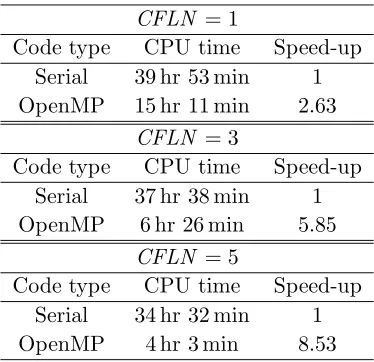
Table 4. Speed-up by the OpenMP code on 32 cores at diﬀerent CFLN.

CFLN = 1

Code type CPU time Speed-up Serial 39 hr 53 min 1 OpenMP 15 hr 11 min 2.63

CFLN = 3

CFLN = 5

memory architecture. In the parallel execution of the code, OpenMP uses the fork-join model as shown in Figure 8. An OpenMP programme begins as a single thread of execution. When it encounters a parallel construct, it creates (‘forks’) the required number of threads and becomes the master thread of all the threads. Programme statements within the parallel construct are executed in parallel by each thread of the team of threads. At the end of the parallel construct, threads synchronize back (‘join’) and only the master thread continues the execution. There can be any number of parallel regions and diﬀerent number of threads in each parallel region, as shown in Figure 8.

Numerical modelling of the human body in the FD-CN-FDTD method, as described in [13, 14], was implemented in OpenMP for the cases ofCFLN = 1, 3 and 5. The geometrical features of the human body were read from a 2-mm resolution male voxel model and for each voxel (representing a certain tissue) the corresponding single–pole Debye parameters were mapped. As the section above the upper chest was modelled, the size of the FD-CN-FDTD computational space was 320×160×220 voxels from the top of the head. The source excitation was z-directed modulated Gaussian pulse centred at 3 GHz. Table 4 shows the achieved improvement by the OpenMP parallelization over the serial code when it was run for 1050/CF LN time steps. With the OpenMP code, the CPU time has been greatly reduced when CFLN = 1 and as expected, the most signiﬁcant reduction in CPU time has been achieved when

CFLN is higher. However, the scaling is not perfect for the number of threads (32) the code uses because in OpenMP, usually, it is hard to obtain perfect speed-ups even when the parallelization is done correctly [15]. Understanding the details of underlaying hardware and using vendor-supplied parallel mathematical operation libraries may improve the performance to some extent.

An interesting observation in Table 4 is the increase of speed-up by OpenMP parallelization at higher CFLN. From the speed-up by OpenMP for CFLN = 1, 3 and 5 are 2.63, 5.85 and 8.53, respectively, it is found that better speed-up always comes at higherCFLN, indicating that the use of the FD-CN-FDTD method is more appropriate while parallelized. This may be resulted from the fact that the operations involved in the increased iteration numbers to converge at higherCFLN, as shown in Figure 6, are possibly more suitable for parallelization.

6. CONCLUSION

(8)

excessively large memory. Therefore, two best-known iterative methods, GMRES and BiCGStab, were studied in terms of the number of iteration requirements for convergence with different CFLN, CPU-time and memory requirements. As in each CPU-time step of the FD-CN-FDTD method, matrix-vector multiplications need to be done repeatedly until the solution converges, it has a significant contribution in the overall computational performance. Also it is found that more iterations are required to converge at higherCFLN which results in increased number of matrix-vector multiplications. Therefore, efficient implementation of matrix-vector multiplications has been studied in order to improve the overall efficiency. FD-CN-FDTD code was parallelized by using OpenMP in shared memory architecture and it was found that better speed-up always comes at higherCFLN indicating that the use of the FD-CN-FDTD method is more appropriate while parallelized.

REFERENCES

1. Taﬂove, A. and S. Hagness, Computational Electrodynamics: The Finite-diﬀerence Time-domain Method, 3rd Edition, Artech House, Boston, MA, 2005.

2. Yang, Y., R. Chen, and E. Yung, “The unconditionally stable Crank Nicolson FDTD method for three-dimensional Maxwell’s equations,” Microwave and Optical Technology Letters, Vol. 48, 1619–1622, 2006.

3. Rouf, H. K., F. Costen, and S. G. Garcia, “3-D Crank-Nicolson ﬁnite diﬀerence time domain method for dispersive media,”Electronics Letters, Vol. 45, No. 19, 961–962, 2009.

4. Rouf, H. K., F. Costen, S. G. Garcia, and S. Fujino, “On the solution of 3-D frequency dependent Crank-Nicolson FDTD scheme,” Journal of Electromagnetic Waves and Applications, Vol. 23, No. 16, 2163–2175, 2009.

5. Joseph, R., S. Hagness, and A. Taﬂove, “Direct time integration of Maxwell’s equations in linear dispersive media with absorption for scattering and propagation of femtosecond electromagnetic pulses,”Optics Letters, Vol. 16, No. 18, 1412–1414, 1991.

6. Crank, J. and P. Nicolson, “A practical method for numerical evaluation of solutions of partial diﬀerential equations of the heat-conduction type,” Mathematical Proceedings of the Cambridge Philosophical Society, Vol. 43, 50–67, 1947.

7. Barrett, R., M. Berry, et al., Templates for the Solution of Linear Systems: Building Blocks for Iterative Methods, SIAM Press, Philadelphia, 1993.

8. Saad, Y. and M. H. Schultz, “GMRES: A generalized minimal residual method for solving nonsymmetric linear systems,”SIAM Journal on Scientiﬁc and Statistical Computing, Vol. 7, 856– 869, 1986.

9. Van der Vorst, H., “BiCGSTAB: A fast and smoothly converging variant of BiCG for the solution of nonsymmetric linear systems,” SIAM Journal on Scientiﬁc and Statistical Computing, Vol. 13, 631–644, 1992.

10. Yang, Y., R. Chen, et al., “Application of iterative solvers in 3D Crank-Nicolson FDTD method for simulating resonant frequencies of the dielectric cavity,” Asia-Paciﬁc Microwave Conference, 1–4, 2007.

11. Numerical Analysis Group, Rutherford Appleton Laboratory Harwell Subroutine Library, (HSL), 2007 for Researchers, http://www.hsl.rl.ac.uk/hsl2007/hsl20074researchers.html.

12. Saad, Y., “SPARSKIT: A basic toolkit for sparse matrix computations (Version 2),” Research Institute for Advanced Computer Science, NASA Ames Research Center, 1994, http://www-users.cs.umn.edu/ saad/software/SPARSKIT/sparskit.html.

13. Rouf, H. K., “Unconditionally stable ﬁnite diﬀerence time domain methods for frequency dependent media,” Ph.D. Thesis, The University of Manchester, UK, 2010.

14. Rouf, H. K., F. Costen, and M. Fujii, “Modelling EM wave interactions with human body in frequency dependent Crank Nicolson method,”Journal of Electromagnetic Waves and Applications, Vol. 25, Nos. 17–18, 2429–2441, 2011.