Western University Western University
Scholarship@Western
Scholarship@Western
Electronic Thesis and Dissertation Repository
1-21-2015 12:00 AM
Development And Study Of Measurement Methods For Jets And
Development And Study Of Measurement Methods For Jets And
Bogging In A Fluidized Bed
Bogging In A Fluidized Bed
Majid Hamidi
The University of Western Ontario
Supervisor Dr. Cedric Briens
The University of Western Ontario Joint Supervisor Dr. Franco Berruti
The University of Western Ontario
Graduate Program in Chemical and Biochemical Engineering
A thesis submitted in partial fulfillment of the requirements for the degree in Doctor of Philosophy
© Majid Hamidi 2015
Follow this and additional works at: https://ir.lib.uwo.ca/etd
Part of the Process Control and Systems Commons
Recommended Citation Recommended Citation
Hamidi, Majid, "Development And Study Of Measurement Methods For Jets And Bogging In A Fluidized Bed" (2015). Electronic Thesis and Dissertation Repository. 2679.
https://ir.lib.uwo.ca/etd/2679
This Dissertation/Thesis is brought to you for free and open access by Scholarship@Western. It has been accepted for inclusion in Electronic Thesis and Dissertation Repository by an authorized administrator of
i
DEVELOPMENT AND STUDY OF MEASUREMENT METHODS FOR JETS
AND BOGGING IN A FLUIDIZED BED
(Thesis Format: Integrated Article)
by
Majid Hamidi
Graduate Program
In
Engineering Science
Department of Mechanical and Materials Engineering
A thesis submitted in partial fulfillment of the requirements for the degree of
Doctor of Philosophy
The School of Graduate and Postdoctoral Studies
The University of Western Ontario
London, Ontario Canada
ii
ABSTRACT
In gas-fluidized processes such as Fluid CokingTM and Fluid Catalytic Cracking, heavy
hydrocarbons are converted to lighter products. In the Fluid Coking process, heavy oil
feed is contacted with hot fluidized coke particles, heats up and undergoes thermal
cracking. If the local concentration of liquid is very high, particles may stick together
which can eventually result in process upset because of poor fluidization or even
defluidization, a condition commonly known in industry as "bogging".
Coke particles in a Fluid Coker have a high dielectric constant and can concentrate an
electric field within themselves. Using a capacitance sensor, the void distribution in a bed
of coke particles can be visualized based on the difference in dielectric constant between
coke particles and the fluidization gas. The voidage fluctuations caused by gas bubbles
have been shown to change dramatically as the bed becomes bogged. Therefore,
capacitance sensors are capable of predicting the bogging condition in fluid cokers.
However, they should be properly designed to account for the bed geometry, the position
of sensors, the temperature and the degree of electromagnetic noise in the area. This was
the primary research objective for this thesis.
The first part of the thesis research focused on designing noiseless capacitance sensors
that can be used to measure the liquid concentration in a fluidized bed as well as bubble
properties and the length of jet cavities. The effect of bogging on the distribution of a
liquid sprayed into fluidized bed was then investigated by determining the impact of
bogging on the breakage rate of the liquid-solid agglomerates that are formed when a
liquid is sprayed into a fluidized bed. Bubble rise velocity and frequency was measured at
different locations of the fluidized bed to understand and predict early bogging.
Pressure measurements are easier to perform in industrial units than capacitance
measurements. The knowledge acquired with capacitance measurements was then
applied to the design of early bogging detection methods from pressure measurements. A
bogging index was proposed; it uses a Kolmogorov-Smirnov test of the wavelet
coefficients of pressure fluctuations and was optimised using a genetic algorithm to
iii
Detection of bogging with acoustic measurements is discussed in the next section. The
speed of sound was measured at different levels of particles cohesiveness and fluidization
velocities. Experimental data was compared with the results of simulations with the
COMSOL acoustic toolbox.
The last part of the thesis applies the new capacitance sensors to the measurement of jet
cavity fluctuations in fluidized beds. Two types of jets were investigated: the supersonic
gas jets used for particle attrition in fluidized beds and the jets formed when liquid is
atomized with a gas into a fluidized bed. Jet fluctuations can cause the erosion of fluidized
bed internals and must be known when designing a fluidized bed. A new correlation was
developed to predict the fluctuations of the jet penetration in fluidized beds. The effect of
bogging on jet fluctuations was also investigated. The results of these experiments were
interpreted with the previously developed correlations.
Keywords:
Fluidized bed, bogging detection, capacitance measurements, agglomerate breakage,
iv
CO-AUTHORSHIP
Chapter 2
Article Title:
A novel Ac-based capacitance sensor with differential noise cancelling
Authors:
Majid Hamidi, Cedric Briens, Franco Berruti, Jennifer McMillan
Article Status:
Unpublished
Chapter 3
Article Title:
Effect of fluidized bed bogging on distribution of sprayed liquid on fluidized particles
Authors:
Majid Hamidi, Cedric Briens, Franco Berruti, Jennifer McMillan
Article Status:
Published
Contributions:
Majid Hamidi conducted all experimental work, data analysis and writing. Cedric
Briens, Franco Berruti and Jennifer McMillan provided guidance, supervision and
revised drafts of the work.
Chapter 4
Article Title:
Early detection of defluidization using wavelet analysis of pressure fluctuations
Authors:
Majid Hamidi, Cedric Briens, Franco Berruti, Jennifer McMillan
v Unpublished
Contributions:
Majid Hamidi conducted all experimental work, data analysis and writing. Cedric
Briens, Franco Berruti and Jennifer McMillan provided guidance, supervision and
revised drafts of the work.
Chapter 5
Article Title:
Early detection of defluidization from measured speed of sound
Authors:
Majid Hamidi, Cedric Briens, Franco Berruti, Jennifer McMillan
Article Status:
Unpublished
Contributions:
Majid Hamidi conducted all experimental work, data analysis and writing. Cedric
Briens, Franco Berruti and Jennifer McMillan provided guidance, supervision and
revised drafts of the work.
Chapter 6
Article Title:
Study of supersonic gas jets fluctuations in a gas-solid fluidized bed with capacitance
sensors
Authors:
Majid Hamidi, Cedric Briens, Franco Berruti, Jennifer McMillan
Article Status:
Unpublished
vi
Majid Hamidi conducted all experimental work, data analysis and writing. Cedric
Briens, Franco Berruti and Jennifer McMillan provided guidance, supervision and
revised drafts of the work.
Chapter 7
Article Title:
Effect of bogging on gas and gas-liquid jet fluctuations
Authors:
Majid Hamidi, Cedric Briens, Franco Berruti, Jennifer McMillan
Article Status:
Unpublished
Contributions:
Majid Hamidi conducted all experimental work, data analysis and writing. Cedric
Briens, Franco Berruti and Jennifer McMillan provided guidance, supervision and
revised drafts of the work.
Contributions:
Majid Hamidi conducted all experimental work, data analysis and writing. Cedric
Briens, Franco Berruti and Jennifer McMillan provided guidance, supervision and
vii
ACKNOWLEDGEMENTS
First, I would like to express my gratitude to my supervisors Dr. Cedric Briens
and Dr. Franco Berruti from the Institute of Chemicals and Fuels from Alternative
Resources (ICFAR) at the University of Western Ontario, for their guidance and support
throughout the completion of my thesis work. Dr. Briens and Dr. Berruti kindly shared
their knowledge and expertise to help on my research work, I am truly thankful for all of
that. I would like to thank Dr. Jennifer McMillan, of Syncrude Canada, for providing me
with valuable feedback and ensuring that my research was industrially relevant. Special
thanks to Rob Taylor for his help on my experimental equipment. I also wish to
acknowledge all my colleagues from ICFAR. It was great to know you all and thank you
for all your help in my research work.
At last, my deepest gratitude goes to my wife, Maryam Mohagheghi Dar ranji, for
her unconditional support and love. I would not have been able to pursue my education in
Canada and complete my PhD degree if you had not always believed in me. I would like
viii
Table of Contents
Abstract ...ii
Co-Authorship ...iv
Acknowledgements ... vii
List of Tables ...xi
List of Figures ... xii
Nomenclature ... xvii
Chapter 1: Introduction ... 1
1.1. Present Thesis Work ... 1
1.2. Fluid Coking Process ... 1
1.3. Problem statement ... 3
2. Choice of measurement techniques and analysis methods ... 4
2.1.a. Electrical Capacitance Tomography ... 4
2.1.b. Pressure measurement ... 6
2.1.c. Acoustic emission ... 9
2.1.d. Temperature measurement ... 10
3. Research Objectives ... 11
4. References ... 12
Chapter 2: A Novel AC-based Impedance Meter to Reduce Capacitive and Inductive Coupling Noise ... 16
2.3. Proposed impedance meter ... 20
2.3.1. Circuit Design ... 20
2.3.2. Effect of capacitive coupling ... 21
2.4. Effect of inductive coupling ... 21
2.5. Disscussion and experimental results ... 23
2.6. Conclusions ... 24
2.7. References ... 25
Chapter3: Effect of Fluidized Bed Bogging On The Distribution of Sprayed Liquid On Fluidized Particles ... 26
3.1. Introduction ... 26
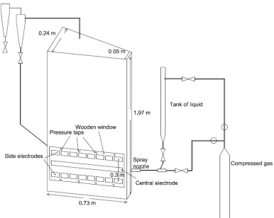
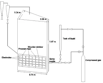
3.2. Experimental Set up ... 27
3.2.1. Equipment and Materials ... 27
3.2.2. Origin of bogging ... 29
ix
3.3. Results And Discussion ... 34
3.3.1. Bogging Condition in the Fluidized Bed ... 34
3.3.2. Effect of Bogging on Bubble Properties ... 35
3.3.3. Results of Experiments with Coke Particles ... 36
3.3.4. Results of Experiments with Sand Particles ... 38
3.4. Conclusions ... 39
3.5. References ... 40
Chapter4: Early detection of defluidization using wavelet analysis of pressure fluctuations ... 42
4.1. Introduction ... 42
4.2. Experimental ... 44
4.2.1. Experimental Setup ... 44
4.2.2. Measuring methods ... 46
4.3. Kinetics of agglomerate breakage ... 46
4.4. Results of previous methods ... 47
4.5. Wavelet analysis of pressure fluctuations ... 51
4.5.1. Wavelet transform ... 51
4.5.2. Optimized bogging index based on wavelet coefficients ... 52
4.6. Results and discussion ... 54
4.7. Comparison of new KS test with other bogging detection methods ... 58
4.8. Effect of bogging on the frequency spectrum of pressure fluctuations .. 60
4.9. Conclusion ... 64
4.10. References ... 64
Chapter 5: Early detection of defluidization from the measured speed of sound 67 5.1. Introduction ... 67
5.2. Speed of sound in the fluidized bed... 68
5.3. Experimental ... 69
5.3.1 Experimental set up ... 69
5.3.2. Measuring the speed of sound ... 71
5.3.3. Measuring the bubble geometry and bubble distance from the wall .. 72
5.4. Results: Measured Speed of Sound ... 75
Interpretation of Results ... 77
5.3.1. The Simulation Approach ... 77
5.3.2. The Wave-Equation For Sound Propagation ... 79
x
Conclusion ... 85
References ... 86
Chapter 6: Study of Supersonic Gas Jets Fluctuations in a Gas-Solid Fluidized Bed with Capacitance Sensors ... 88
6.1. Introduction ... 88
6.2. Experimental ... 90
6.2.1. Experimental Setup ... 90
6.2.2. Measurement of Local Voidage ... 92
6.2.3. Pre-Test Imaging Experiments ... 93
6.2.4. Measurement of Jet Length ... 93
6.2.5. Measurement of Bubble Velocity ... 94
6.3. Results and Discussion ... 95
6.3.1. Study of Supersonic Jet Penetration Length ... 95
6.3.2. Study of fluctuations of the supersonic jet length... 100
6.3.3. Empirical correlation for supersonic jet fluctuations ... 106
6.4. Conclusions ... 107
6.5. References ... 108
Chapter 7: Effect of bogging on gas and gas-liquid jet fluctuations ... 110
7.1. Introduction ... 110
7.2. Experimental ... 111
7.2.1. Experimental set up ... 111
7.2.2. Measurement of Local Voidage ... 114
7.2.3. Measurement of jet length ... 114
7.3. Distribution of Jet length ... 115
7.4. Results and Discussion ... 116
7.4.1. Effect of Bogging on Gas Jet Length ... 116
7.4.2. Effect of Bogging on Gas-Liquid Jet Length ... 121
7.4.3. Effect of Bogging on the Frequency of Jet Fluctuations ... 125
7.5. Conclusion ... 127
7.6. References ... 127
Chapter 8: CONCLUSIONS AND RECOMMENDATIONS ... 129
8.1. Conclusions ... 129
8.2. Recommendations ... 130
Appendix A ... 131
xi
VITAE ... 134
LIST OF TABLES
Table 4.1: Exponents of wavelet coefficients at each octave calculated with Genetic algorithm ... 54Table 4.2: Exponents of wavelet coefficients at dominant octaves calculated with Genetic algorithm ... 54
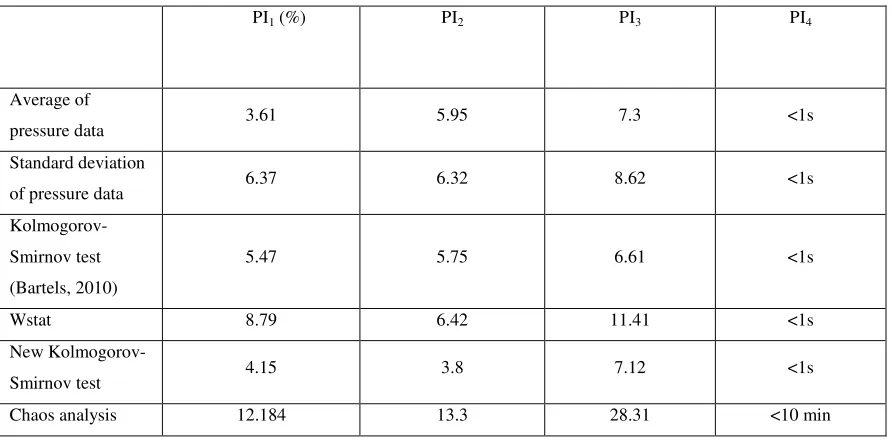
Table 4.3: Comparison of bogging detection methods ... 60
Table 5.1: Speed of sound calculated with different assumptions ... 69
xii
LIST OF FIGURES
Figure 1.1: The fluid coking process (adapted from House, 2007) ... 2 Figure 2.1: Auto balancing bridge circuit... 17 Figure 2.2: Capacitive coupling between a conductor and ... 18 Figure 2.3: Inductive coupling between a conductor and auto balancing bridge circuit ... 18 Figure 2.4: Equivalent circuit for the inductive coupling ... 19 Figure 2.5: Proposed impedance meter... 20
Figure 2.6: Capacitive coupling between a conductor and Proposed impedance meter ... 21
Figure 2.7: Inductive coupling between a conductor and
Proposed impedance meter ... 22 Figure 2.8: Equivalent circuit for Inductive coupling between a conductor and... 22 Proposed impedance meter ... 22 Figure 2.9: Power spectrum of output signal of a- auto balancing bridge b- novel impedance meter ... 23 Figure 2.10: Theoretical and experimental values for a) amplitude of the
impedance versus frequency b)phase of the impedance versus frequency ... 24 Figure 3.1: Schematic of experimental set up ... 27 Figure 3.2: Average pressure gradient measured between two taps at heights 0.05 m and 0.45 m above the gas distributor versus mass fraction of Glycerol and Voltesso oil ... 30 Figure 3.3: Calibration curve ... 32 Figure 3.4: The mass of total Varsol freed from agglomerate versus time ... 33 Figure 3.5: Effects of Voltesso oil mass fraction on natural frequency of
agglomerate breakage for various fluidization velocities during liquid injection .. 34 Figure 3.6: a) bubble crosses the electric field of three electrodes b) The effect of crossing on capacitance signals – calculation of bubble rise time ... 36 Figure 3.7: Effects of fluidization velocity and oil mass fraction on average bubble velocity ... 37 Figure 3.8: Effects of fluidization velocity and oil mass fraction on standard
xiii
Figure 4.2: Differential pressure data measured between two vertically separated
pressure tapes at a) Normal operation b) Initial point of bogging ... 47
Figure 4.3: Average and standard deviation of measured pressure versus oil mass fraction and fluidization velocity ... 48
Figure 4.4: Kolmogorov-Smirnov statistic (Bartels, 2010) of measured pressure versus oil mass fraction and fluidization velocity after injection ... 49
Figure 4.5: Wstat of measured pressure versus oil mass fraction and fluidization velocity ... 49
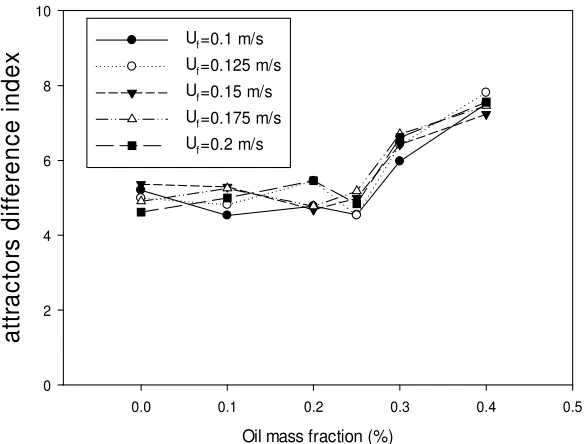
Figure 4.6: Attractors difference index versus oil mass fraction and fluidization velocity (measured pressure at dry bed is the reference ... 50
Figure 4.7: New ideal bogging index ... 53
Figure 4.8: New Kolmogorov-Smirnov statistic versus oil mass fraction and fluidization velocity ... 55
Figure 4.9: New Kolmogorov-Smirnov statistic versus oil mass fraction a) at different length of data (Uf=0.1 m/s) b) at different fluidization velocities for 2 minutes of pressure data ... 55
Figure 4.10: Kolmogorov-Smirnov statistic (Bartels, 2010) of measured pressure versus oil mass fraction a) at different length of data (Uf=0.1 m/s) b) at different fluidization velocities for 2 minutes of pressure data ... 56
Figure 4.11: Wstat of measured pressure versus oil mass fraction a) at different length of data (Uf=0.1 m/s) b) at different fluidization velocities for 2 minutes of pressure data ... 57
Figure 4.12: Attractors difference index versus oil mass fraction at different length of data (Uf=0.1 m/s) ... 57
Figure 4.13: New Kolmogorov-Smirnov statistic versus oil mass fraction and fluidization velocity a) The reference data measured at 0.1% oil fraction b) The reference data measured at 0.2% oil fraction ... 58
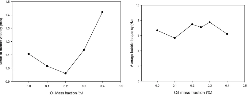
Figure 4.14: Average bubble velocity and frequency at different Voltesso oil mass fractions (Uf=0.1 m/s) ... 61
Figure 4.15: Measured acoustic intensity generated by subwoofer in air ... 62
Figure 4.16: Measured acoustic intensity generated by subwoofer in a fluidized bed of dry or wet coke particles ... 62
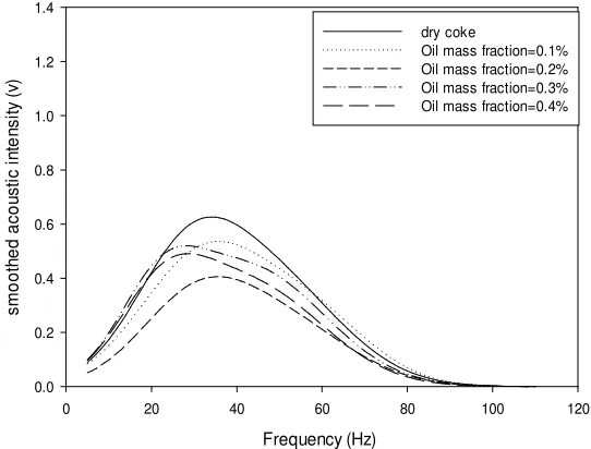
Figure 4.17: Smoothed acoustic intensity generated by subwoofer in a fluidized bed of dry or wet coke particles ... 63
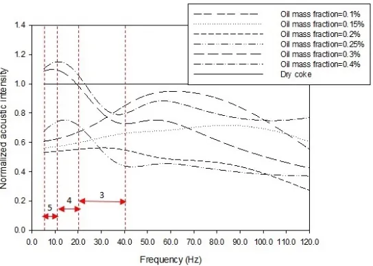
Figure 4.18: Normalized acoustic intensity generated by subwoofer in a fluidized bed of dry or wet coke particles (Octaves 3,4 and 5 are labeled) ... 64
Figure 5.1: Schematic diagram of experimental set up ... 71
Figure 5.2: 250 Hz train pulses of sound generated by speaker ... 71
xiv
Figure 5.4: Time series of simulated normalized capacitance at different bubble height when the bubble frontal diameter is 8 cm and the bubble distance from the
wall ranges from 4 cm to 6 cm ... 73
Figure 5.5: a) Normalized capacitance in amplitude b) Normalized capacitance in amplitude and time, showing the 18 points used as input to the neural network 74 Figure 5.6: Outputs of neural networks versus targets for all the simulated data ... Show dashed lines e.g. + 10 % and – 10% ... 74
Figure 5.7: Measured speed of sound at different superficial gas velocities measured at four horizontally separated locations ... 76
Figure 5.8: Measured speed of sound at different oil mass fractions and fluidization velocities measured at four horizontally separated locations ... 76
Figure 5.9: a) Effect of fluidization velocity on the bubble frequency b) Effect of fluidization velocity on the bubble frontal diameter c) Effect of fluidization velocity on the bubble aspect ratio ... 77
Figure 5.10: a) Effect of oil mass fraction on the bubble frequency b) Effect of oil mass fraction on the bubble frontal diameter c) Effect of oil mass fraction on the bubble aspect ratio ... 78
Figure 5.11: Local acceleration of particles at microphone location simulated with COMSOL using a bubble with a height of 8 cm and a frontal diameter of 6 cm, located 5 cm far from the wall ... 81
Figure 5.12: Simulated speed of sound versus bubble distance from the wall ... 82
Figure 5.13: Simulated speed of sound versus bubble height and bubble frontal diameter ... 82
Figure 5.14: Measured speed of sound versus predicted speed of sound from the model Remove error bars, add dashed curve ... 84
Figure 5.15: Normalized simulated capacitance versus normalized time- Dash line when a bubble with frontal diameter of 6 cm and height of 8 cm is passing- Continuous line when another bubble with frontal diameter of 6 cm and height of 4 cm is passing beside the first bubble ... 85
Figure 6.1: Experimental set up ... 90
Figure 6.2: Laval type nozzle, dth =2.4 mm ... 91
Figure 6.3: Laval type nozzle, dth =2.8 mm ... 91
Figure 6.4: configuration of electrodes ... 91
Figure 6.5: Average normalized capacitance of 30 electrodes versus the average bed voidage measured with pressure transducers ... 93
Figure 6.6: Image of the void tube acquired with capacitance sensors ... 93
xv
Figure 6.8: Comparison between measured supersonic jet penetration depth and
correlations ... 96
Figure 6.9: Jet penetration length versus gas mass flux for different nozzle diameters ... 96
Figure 6.10: Jet penetration length versus gas mass flux for different gas densities ... 97
Figure 6.11: Jet penetration length versus gas mass flux ... 98
for different fluidization velocities ... 98
Figure 12: Jet penetration length versus gas ... 98
Figure 6.13: Comparison between values predicted with Benjelloun’s correlation and all measured horizontal supersonic jet lengths at different nozzle sizes, nozzle mass flowrates and nozzle gas densities ... 99
Figure 6.15: q-q plot of jet penetration length distribution at constant nozzle mass flowrate :(1), (2), (3) with horizontal nozzle and Uf = 0.1, 0.2, 0.3 m/s and (4), (5) with inclined nozzle α=15o,-150 while Uf = 0.1m/s ... 101
Figure 6.16: Cross correlation between voidages of horizontal supersonic jet and voidages measured with electrodes below the jet with different horizontal distance ... 102
Figure 6.17: Maximum cross correlation between voidages of horizontal supersonic jet and voidages measured with electrodes below the jet versus horizontal distance from nozzle tip (Uf = 0.1 m/s; Nitrogen injected with horizontal nozzle with do = 2.4 mm) ... 103
Figure 6.18: Coefficient of variation of supersonic jet length versus nozzle thrust and nozzle inclination angle ... 104
Figure 6.19: Coefficient of variation of horizontal supersonic jet length versus fluidization velocity and nozzle thrust ... 105
Figure 6.20: Bubble velocity with 95% confidence interval versus fluidization velocity ... 106
Figure 6.21: Coefficient of variation of supersonic jet length versus nozzle thrust with different injection gases and nozzle diameters ... 106
Figure 6.22: Predicted CV of supersonic jet versus measured CV of supersonic jet at different nozzle thrust, nozzle inclination angles and fluidization velocities ... 107
Figure 7.1: Experimental set up ... 112
Figure 7.2: Laval type nozzle, dth =2.4 mm ... 112
Figure 7.3: Laval type nozzle, dth =2.8 mm ... 113
Figure 7.4: Schematic of Spray nozzle ... 113
xvi
Figure 7.6: Average length of gas jet versus mass fraction of Voltesso oil at different fluidization velocities ... 116 Figure 7.7: Particle bulk density versus mass fraction of Voltesso oil at different fluidization velocities ... 117 Figure 7.8: Comparison of measured and expected average gas jet length at different fluidization velocities ... 118 Figure 7.9: CV of gas jet length versus mass fraction of Voltesso oil at different fluidization velocities ... 119 Figure 7.10: Bed pressure drop versus superficial gas velocity at different
concentrations of Voltesso oil ... 119 Figure 7.11: Complete and minimum fluidization velocity at different
concentrations of Voltesso oil ... 120
Figure 7.12: Comparison of measured and expected CV of gas jet length at different fluidization velocities ... 121
Figure 7.13: Gas-liquid jet length versus time at different concentrations of
Voltesso oil (Uf=0.1 m/s) ... 122
Figure 7.14: Average length of gas-liquid jet versus mass fraction of Voltesso oil at different fluidization velocities ... 123 Figure 7.15: Measured mass of free injected Varsol liquid versus mass fraction of Voltesso oil at different fluidization velocities ... 123 Figure 7.16: CV of length of liquid-gas jet versus mass fraction of Voltesso oil at different fluidization velocities ... 124 Figure 7.17: Comparison of measured and expected CV of liquid-gas jet length at different fluidization velocities ... 125 Figure 7.18: Frequency of fluctuations of gas jet and gas-liquid jet length at
different Voltesso oil mass fractions (Uf=0.1 m/s) ... 126
xvii
NOMENCLATURE
A Approximation wavelet component
A Wavelet scale
A Cross section area of nozzle exit (m2)
a Particle acceleration, m/s2
a Characteristic dimension, m
B Bogging index
c Speed of sound, m/s
Cij Capacitance (F)
D Effective electric field length, m
D Bed hydraulic diameter (m)
D Detail wavelet component
d Bubble distance from the wall, cm
d Distance between two sources, m
d Particle Sauter mean diameter (m)
d Nozzle exit diameter (m)
d Nozzle throat diameter (m)
F Thrust of the nozzle (N)
g Normalized total free liquid GLR Gas-to-liquid ratio, wt% H Static bed height (m)
xviii
In Electrical current (A)
M Total mass, kg
m Level of oil mass fraction
m0 Nozzle mass flowrate (kg/s)
n Level of fluidization velocity
nw Number of wavelet octaves
p Pressure at nozzle throat (Pa)
p Pressure at nozzle exit (Pa)
Q Monopole acoustic source, N/m.kg
R Gas constant, J/mol.K
Rx Electrical resistance (Ω)
SNRout Signal to noise ratio at output
T Temperature, K
t Time, s
Us Speed of sound in particles, m/s
U0 Speed of sound in ideal gas, m/s
U3 Fluidization velocity (superficial gas velocity), m/s
U3 Fluidization velocity (m/s)
U43 Minimum fluidization velocity (m/s)
U Gas velocity at nozzle exit (m/s)
V Source voltage (V)
V Output voltage (V)
xix
X Mass concentration of free liquid on a dry solids basis, wt%
z Height from gas distributor (m)
Z Specific acoustic impedance, Ns/m3
Z8 Electrical impedance (Ω)
α Natural frequency of agglomerate breakage, Hz
α: Nozzle inclination angle (degree)
γ Ratio of specific heat constants
γ Power of wavelet octave
ϵ Voidage
v Particle velocity, m/s
ξ Particle displacement, m
ρ Density, kg/m3
ρ Gas density at nozzle exit (kg/m3)
ρ3 Fluidization gas density (kg/m3)
ρ? Gas density, kg/m3
ρ Particle density, kg/m3
Ψ Mother wavelet function
xx
SUBSCRIPTS
br breakage
cal calculated
L injected liquid
S dry coke
1
CHAPTER 1: INTRODUCTION
1.1. Present Thesis Work
Fluidized beds have been in use for decades and have been applied to numerous
industries due to their excellent gases and solids mixing, and rapid mass and heat transfer.
Fluid Coking as an application of fluidized beds is a continuous process for heavy oil
upgrading. The main objective of the thesis is to develop a method to detect early
bogging in the Fluid Coking process, using non-invasive methods that can be used in
industrial fluidized bed. Analysis of the effect of bogging on jet penetration and its
fluctuations is the other objective of the thesis.
After a general introduction to the Fluid Coking process, this chapter reviews
published, experimental studies on bogging detection in fluidized beds. The research
objectives of this thesis are then presented.
1.2. Fluid Coking Process
Canada has the third largest oil reserves in the world behind Saudi Arabia and
Venezuela. Out of the total oil reserves, 170 billion barrels are bitumen from the oil sands,
which are currently recoverable and are located in Alberta (Syncrude Canada, 2011). Oil
sands contain a mix of clay material, water and a form of heavy oil called bitumen.
Bitumen, in its raw form is a dark-colored, asphalt-like oil, that requires upgrading to
enable its transportation by pipeline and to be used by conventional refineries.
Heavy oil such as bitumen can be upgraded into synthetic crude oil using Fluid
CokingTM which is a thermal, non-catalytic conversion process. Fluid Coking is prefered
for upgrading bitumen because of its high flexibility, reliability, continuous operation and
low greenhouse gas emissions. Syncrude Canada Ltd. has the three largest Fluid Cokers
in the world and is one of the largest producers of crude oil in Canada (Syncrude Canada,
2
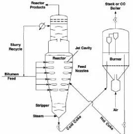
The Fluid Coker that is used by Syncrude Canada is a two vessels system,
including a fluidized bed burner and a fluidized bed reactor, as shown in Figure 1.1
(House, 2007).
Figure 1.1: The fluid coking process (adapted from House, 2007)
During the process, the fluidized bed burner heats up coke particles to temperatures
ranging from 600 to 680 °C while they are transported to the top of the reactor section
where they are contacted with bitumen feed, at a temperature ranging from 300 to 400°C.
The coker reactor as the primary equipment in the bitumen upgrading can be divided into
three sections: stripper section, reaction section and scrubber section. There are some
liquid-gas nozzles in the reaction section to atomize the bitumen and to quickly and
uniformly spray it over the individual particles for a stable reaction rate. In the Syncrude
fluid coker, these spray nozzles use 600 psig steam to atomize and spray the bitumen into
the reactor dense coke bed. Bitumen then thermally cracks on the surface of the hot coke
particles, at a temperature ranging from 510 to 550 °C. Vapours released from the
3
to remove the entrained coke particles which are sent back to the dense bed into the
stripper section. The average superficial velocity of the rising gases is ranging from 0.3
m/s to 1.0 m/s depending upon the coke size to maintain fluidization (Pfeiffer,
1959).After passing the cyclones, the released vapours flow through the condenser to be
processed into the shipping section downstream. Coke particles losing heat in the
cracking process move down the reactor and circulate back to the reactor after reheating
in the burner.
1.3. Problem statement
Industrial fluidized beds are often used for continuous operation, with particles added to
or removed from the fluidized bed continuously. In a continuously operating fluidized
bed, alteration of hydrodynamic behaviour may occur over time due to imposed or
unwanted changes. Changes in fluidization velocity or particle size distribution are
examples of imposed changes. Unwanted changes are usually due to formation of
cohesive particles, agglomeration or sintering of particles. Formation of cohesive
particles can be a serious problem in processes such as thermal cracking of bitumen to
naphtha, drying of freshly produced polymers or food and coating of particles for
pharmaceutical use. The problem can be worse if the liquid feed rate is sufficiently high
that it can result in process upset and defluidization, a condition commonly known in
industry as bogging. In Fluid Cokers, bogging can lead to complete unit shut down and
clean-out. Therefore, it is important to detect early bogging to prevent unit upset and shut
down.
Bogging is a gradual phenomenon. In a wet bed, the minimum liquid concentration above
which bed bogging occurs depends on each practical application. The distribution of
injected liquid on fluidized coke particles is critical to the operation of commercial Fluid
Cokers (Briens, 2003). It is important to determine how bogging can impact this
distribution. Therefore, the characterization of early bogging by directly investigating its
impact on the breakage kinetics of the wet agglomerates is of crucial importance and very
4
Bogging also affects the liquid feed jet length and fluctuations in the fluidized bed and
results in less liquid-solid mixing. The analysis of the effect of bogging on gas jet and gas
liquid jet length and fluctuations is also important to determine the impact of bogging on
liquid-solid mixing and yield of the reaction especially in Fluid Cokers.
2. Choice of measurement techniques and analysis methods
In methods reviewed in this section, one or more process parameters are measured during
fluidized bed operation. These methods could, therefore, be applied as an online bogging
detection system.
Other methods have been published that could not be applied to the routine monitoring of
commercial reactors. Positron Emission Particle Tracking (Bridgwater, 2004) is based on
tracking a radioactive particle coated with a positron emitter tracer and requires adding
radioactive particles to the bed. The “falling ball method” (McDougall, 2005) in which
the velocity of a ball falling from the top to the bottom of the bed is measured,
characterizes the fluidity of the fluidized bed.
In contrast, most of the bogging detection methods that have been proposed in the
literature are concerned with the measurement of process variables that can be applied to
large industrial fluidized beds. Examples of these methods are measurement of
temperature or pressure (Werther, 1999). In addition, the capacitance measurement based
on the designed noiseless circuit described in chapter 2, could also be applied to industrial
fluidized beds.
2.1.a. Electrical Capacitance Tomography
Electrical capacitance tomography (ECT) is a measurement method based on the change
in the electrical capacitance due to variations in the distribution or concentration of
dielectric materials in a given volume. Using the measured capacitance, an image of
material distribution can be reconstructed. compared with other tomography methods,
ECT is fast (300 frames/s was used in this thesis), low cost, non-invasive, without
radiation and can withstand high temperature and pressure in the fluidized bed. The
5
circuits with advantages and disadvantages associated with each of those (Yang, 1996).
ECT can be used to monitor different processes including fluidized beds, fluidized bed
dryers, gas-solids pneumatic conveying and gravity flows. No studies has been reported
using ECT directly for bogging detection but there are publications, reviewed below, in
which ECT has been applied to identify flow dynamics and liquid concentration that are
closely related to bogging.
2.1.a.1. Flow dynamics measurements
Wang et al. studied bubbling and slugging flow regimes in a circulating fluidized bed
with a square cross-sectional area using the ECT technique (Wang, 2006). The frequency
spectrum, probability density function, and autocorrelation function of the solid holdup
fluctuations as well as bubble diameter were calculated under different regimes to
investigate chaotic particle behaviours in the fluidized bed. The dominant frequency of
bubbles near the wall and near the center of the bed was also obtained by fitting the
power spectra as power-law.
Zhao et al. used ECT sensors to obtain the solids distribution in a downflow fluidized bed
equipped with specially designed solid distributor (Zhao, 2010). Using reconstructed
images, the spatial and temporal characteristics of solids distribution were calculated.
Their results showed that their new distributor provided a more uniform solids
distribution at the inlet of the downer.
Du et al. analysed and monitored flow dynamics of fluidized beds using the ECT
technique (Du, 2004). Choking phenomenon in a circulating fluidized bed for group A
and B particles was studied. Using 3D ECT to study solid distribution of FCC catalyst
particles (group A particles) in the riser, they found that when the air velocity was lower
than the transport velocity, there were double solids ring flow structure and three-region
flow structure (solids cluster at the core, solids ring close to the wall and a dilute gas ring
region between them). When the air velocity was increased, during choking transition, the
solids cluster in the center disappeared suddenly and the flow structure changed to
two-region flow (dilute phase at the core and dense phase at the wall two-region). For sand
6
slugs and gas intervals were formed, whereas at higher air velocity, open slugs with
particle clusters inside them were observed in the riser.
The studies cited above showed that the ECT technique is a robust method for analysis of
material distribution and its movement in a fluidized bed. The technique can therefore be
used to measure bubble properties and to detect defluidization in a fluidized bed.
2.1.a.2. Liquid concentration measurements
ECT has been used to detect rapid changes in the hydrodynamic regime of dryers.
Chaplin et al. utilized an ECTmethod to measure moisture content in a fluidized bed
dryer (Chaplin, 2005). Results were validated with X-Ray tomography that showed that
the ECT data were fairly accurate when the moisture content was less than 5 wt%.
Wang et al. utilized ECT for online monitoring of solids moisture in a batch fluidized bed
(Wang, 2009). They found that the moisture content only affected the adjacent electrodes.
With compensating the measurement error caused by temperature variations, operation
efficiency was improved with applying a single closed loop control strategy to process
where the data from ECT was used to control actuators.
In summary, the ECT technique was shown to detect local concentration of liquid in the
fluidized bed when there was a considerable difference between the dielectric constant of
the liquid and the dielectric constant of the other materials.
2.1.b. Pressure measurement
Differential and absolute pressure measurements are the most frequently measured and
analyzed parameters influidized beds. Pressure reflects closely the hydrodynamics of
fluidized beds. The analysis method can be categorized as linear or non-linear methods.
Average pressure drop measurements provide information on global properties of a
fluidized bed such as bed height and density while the high frequency components of
measured pressure yield useful information on flow characteristics in the fluidized bed.
2.1.b.1. Linear methods
Kai et al. analysed the average deviation of differential pressure fluctuations (standard
7
measured as well using an optical probe in the bed. They observed that the standard
deviation of differential pressure fluctuations was correlated with fluidization regime and
fluidization quality when fluidization quality was decreasing as the bubble size was
increasing. However, the signal was strongly correlated with fluidization velocity as well.
The variance of high-frequency pressure fluctuations was used for bogging warning
(Chirone, 2006). A steady decrease in variance of high-frequency (100 Hz) pressure
fluctuations observed during combustion of pine seed shells in fluidized beds with
internal diameters of 10 and 37 cm. However, the effect of changes in fluidization
velocity on this method was unknown.
Daw et al. patented a technique called “Fluidization quality analyzer” to determine
fluidization quality by measuring high-frequency pressure drop over the whole or part of
the fluidized bed (Daw, 1995). The pressure signal was amplified by a “buffer amplifier”
and processed by a low-pass filter, a differentiator, a rectifier and a PID-controller that
compared the signal to a predefined set point and regulated a control valve to adjust the
gas flowrate being fed to a fluidized bed. The system was not designed directly to detect
bogging but has potential for bogging detection.
To sum up, methods based on the standard deviation of pressure or high-frequency
component of a pressure signal can indicate the bogging phenomena. However, these
methods are not only sensitive to the fluidization quality, but also to changes in the
fluidization velocity (Van Ommen, 1999). This drawbackposes a problem for robust
implementation of these methods in industrial fluidized beds where fluctuations in the
fluidization velocity are common.
2.1.b.2. Non-linear methods
Many non-linear analysis methods have been developed based on the so-called
state-space projection. In general, at a certain time, the state of a dynamical system such as a
fluidized bed can be determined by projecting all state variables of the system into a
multi-dimensional space. A set of successive states of the system during its evolution in
time is called the “attractor”. The attractor is often considered as the characteristic
8
variable can, theoretically, reconstruct the dynamic state of the system (Takens, 1981).
Using time-delay coordinates, it is possible to convert the time series of local pressure in
the fluidized bed to delay vectors that can be seen as characteristic measure of the
hydrodynamics of the fluidized bed (Takens, 1981). The “bin method” (Fuller, 1993),
“symbol statistics method” (Daw, 1998), “attractor properties method” (van der Stappen,
1993) and “attractor comparison method” (van Ommen, 2000) are nonlinear pressure
analysis methods that have been proposed to detect bogging based on space state
projection. The “attractor comparison method” was shown to be insensitive towards
effects other than bogging within specific limits.
Some studies have proposed statistical methods that are based on the statistical distance
between the probability distribution of a reference pressure signal and the pressure signal
at the current state of the fluidized bed. The Kullback-Leibler distribution distance
(Gheorghiu, 2004) and the Kolmogorov–Smirnov statistic (Bartels, 2010) were proposed
based on this analysis method to detect early bogging in a fluidized bed. Both methods
were able to detect early agglomeration in the fluidized bed. While the sensitivity of the
Kullback-Leibler method to fluidization velocity was not discussed in the publication, a
comparison of the probability distribution of pressure signal based on
Kolmogorov-Smirnov test was shown not to be sensitive to changes in the fluidization velocity. The
reference probability distribution of pressure fluctuations need to be measured during the
normal, desired operating condition of a fluidized bed, which is unfortunately not a
constant condition in industrial fluidized beds.
The W-statistic method proposed by McDougall et al. is based on high frequency
pressure fluctuation measurements in the fluidized bed to detect early bogging
(McDougall, 2005). The underlying rationale is that in the poor fluidity condition, the
fluidized bed transmit pressure fluctuations less well than a well-fluidized bed. Small
pressure fluctuations can be considered the result of pressure waves transmitted from
events far from the pressure tap, while large fluctuations are assumed to result primarily
from local events. The small pressure fluctuations are calculated by subtracting from the
raw signal, a signal smoothed using a wavelet transform of the raw signal. The method
could detect early bogging with different liquid sprayed into a fluidized bed of coke
9
bed where coke particles were fluidized with steam and heavy oil was the liquid sprayed
into the bed. The effect of changes in fluidization velocity was not investigated.
In summary, non-linear analysis methods of pressure measurements received great
attention in the reviewed publications. Attractor comparison and Kolmogorov–Smirnov
test were shown to be insensitive to effects other than agglomeration.
2.1.c. Acoustic emission
Acoustic emissions refer to pressure waves with a specific frequency range that are
emitted from a fluidized bed. They can therefore be considered as shift of pressure
measurements to a higher frequency range and relevant to bogging in the fluidized bed.
Fluidized rigid particles emit sound when they collide with each other. For single size
spherical particles, the generated fundamental frequencies and their harmonics can be
calculated using equation of motion for isotropic elastic spheres. When two spheres with
different diameters collide, the low frequency component of so-called “beat frequencies”
results from the interference of their two fundamental frequency signals. Collision of
particles with a Gaussian size distribution results in a distribution of frequency
differences that causes characteristic beat frequency patterns. Leach et al. showed that
beat patterns are linearly correlated with particle size and the mean frequency can be used
to detect changes in particle size distribution and agglomeration (Leach, 1978).
Zukowski directly evaluated the amplitude of the acoustic emission signal during the
combustion of gaseous fuels in a bubbling fluidized bed of inert particles. Sound waves
with frequencies within the audible range were measured by a microphone placed outside
the fluidized bed (Zukowski, 1999). The mean intensity of the acoustic signal was found
to correlate with bed temperature. A low amplitude signal was observed when the process
was relatively smooth at higher temperature in the range of 950 oC. The amplitude of the
signal was higher at lower temperature when exploding bubbles were the dominant
acoustic source. The work isn’t directly related to bogging detection but made it is clear
that acoustic signals contain valuable information about the bubbling behaviour in the
10
Book et al. used two microphones and an accelerometer to determine the fluidization
quality of a large scale gas–solid fluidized bed of particles, using multi-linear and power
law regressions of traditional (Fourier analysis) and advanced (wavelet decomposition)
signal analysis. The measurements were well correlated to physical measurements of
fluidization quality in the bed (Book, 2011).
Principal component analysis (PCA) has also been used to analyseacoustic measurements
in fluidized beds (Halstensen, 2006). High-temperature accelerometers were installed at
different locations of a urea granulator to measure the sound waves. The process was
monitored using the score-plot for the first two principal components of the measured
signal. The method was capable of detecting unwanted lump-formation in the bed about
30 minutes in advance.
Wang et al. used chaos analysis to detect bogging in a fluidized bed (Wang, 2009). The
signal measured by acoustic emission sensors was first divided into micro-, meso-, and
macroscales by wavelet transform. A coefficient of malfunction was then defined based
on Kolmogorov entropy and correlation dimension, which are measures of
unpredictability of the signal. The proposed coefficient of malfunction was found tobe
sensitive to bogging. However, the method could detect bogging in the fluidized bed only
after formation of cohesive particles.
To sum up, acoustic emissions from fluidized bed processes have been used to determine
the fluidization state and bogging. However, it is still not clear if this method can detect
early bogging. Since other acoustic sources can affect the signal, one has to carefully
select the measuring equipment and location to avoid irrelevant sound emissions (Chen,
2005).
2.1.d. Temperature measurement
Temperatures are often measured in fluidized beds (Werther, 1999). In some fluidized
bed processes, temperature signals carry information on the level of mixing of the bed, i.e.
how quickly differences among local measured temperatures disappear. Temperature
measurements are generally more localized with smaller temporal resolution compared to
11
Lau and Whalley developed a method to detect bogging based on the temperature
difference between two radial locations in a batch fluidized bed of caking coals (Lau and
Whalley, 1981). Since sticky bed material slowed down bed circulation, the thermal
boundary surface shifted away from the wall toward the center of the fluidized bed. The
temperature difference between two radially separated points was measured with a
differential thermocouple (DT). One thermocouple mounted at the center of the bed and
the other one was close to the wall. The temperature difference as well as the variance of
local temperature was higher at lower bed fluidity so the method was able to detect
bogging. However, the temperature difference was also sensitive to fluidization velocity.
Scala et al. proposed a method based on the variance of the measured temperature as well
as the vertical temperature difference in a fluidized bed (Scala, 2006). Both of these
parameters are influenced by the extent of mixing of particles in the fluidized bed. A
laboratory-scale bubbling fluidized bed of silica sand equipped with electrical heaters was
used for their experiments. During the experiments, operating conditions of the bed were
held constant until defluidization occurred. The variance of the temperature signal
measured by the upper probe decreased as it approached the initial point of defluidization
while the normalized relative temperature difference increased at the same time. The
results looked promising in terms of detection of bogging. However, the influence of
fluidization velocity was not investigated.
In summary, the temperature uniformity is closely related to the fluidization quality. A
decrease in the bed fluidity causes the temperature difference between different locations
of the bed to increases while the variance in local temperatures decreases at the same time.
The methods seem promising for detecting early bogging but variations in the fluidization
velocity can make those methods problematic in industrial applications.
3. Research Objectives
This research work aimed at developing robust methods for detecting early bogging
in industrial fluidized beds. In addition the work investigate the effect of bogging on gas
12
The objective of the first study was provide basic measurement tools that could be used in
the rest of the thesis. A noiseless capacitance sensor was developed for void and liquid
measurements in a fluidized bed.
The objective of the second study was to develop a non-invasive technique to detect early
bogging in a fluidized bed based on capacitance measurements. Early bogging condition
is defined from its impact on the breakage of wet agglomerates which is an inherent
characteristic of the solid and liquid interaction. To provide basic information for the rest
of the thesis, the impact of bogging on bubble properties was also studied.
The objective of the third study was to develop a method based on pressure
fluctuations to detect early bogging. The objective of the fourth study was to investigate
and model the impact of bogging on the speed of sound in the fluidized bed, and relate it
to observed changes in bubble properties.
The objective of the fifth study was to measure the fluctuations of the penetration depth
of supersonic jets in fluidized beds. A jet length correlation was also be developed.
The objective of the sixth study was to investigate the effect of bogging on the
fluctuation of gas and gas liquid jets at different gas to liquid ratios and fluidization
velocities.
4. References
Bartels, M. Nijenhuis, J. Kapteijn, F. Van Ommen, .J.R. “Case studies for selective
agglomeration detection in fluidized beds: Application of a new screening methodology”
Powder Technology 2010, 203(2):148-166.
Book G, Albion K, Briens L, Briens C, Berruti F, “On-line detection of bed fluidity in
gas–solid fluidized beds with liquid injection by passive acoustic and vibrometric
methods”, Powder Technology. 2011, 205: 126–113.
Bridgwater J, Forrest S, Parker DJ. “PEPT for agglomeration?” Powder Technology,
13
Briens C, McDougall S, Chan E. "On-line detection of bed fluidity in a fluidized bed
coker" Powder Technology. 2003, 138(23): 160-168.
Chaplin G, Pugsley T, van der Lee L, Kantzas A, Winters C, “The dynamic calibration of
an electrical capacitance tomography sensor applied to the fluidized bed drying of
pharmaceutical granule”, Meas. Sci. Technol. 2005,16:1281–1290.
Chen G, Parsa V, Briens L, Briens C, Smith R, “Application of Adaptive Noise
Cancellation to Acoustic Emissions of A Rotary Dryer”, “Acoustics Week in Canada”,
London, Canada, October 12 - 14, 2005.
Chirone R, Miccio F, Scala F. “Mechanism and prediction of bed agglomeration during
fluidized bed combustion of a biomass fuel: effect of the reactor scale”, Chem Eng J.
2006, 123(3):71–80.
Daw CS, Finney CEA, Nguyen K, Halow JS. “Symbol statistics: a new tool for
understanding multiphase flow phenomena”, In: Nelson Jr RA, Chopin T, Thynell ST,
editors. Proceedings of the ASME heat transfer division, vol. 5. New York: ASME; 1998.
p. 221–9.
Daw CS, Hawk JA; US Deptartment Energy (USAT). “Fluidisation quality analyser for
fluidised beds” Patent US5435972A, 1995.
Du B, Fan L.S, “Characteristics of choking behavior in circulating fluidized beds for
group B particles”, Ind. Eng. Chem. Res. 2004, 43:5507–5520.
Du B, Warsito W, Fan L.S, “ECT studies of the choking phenomenon in a gas–solid
circulating fluidized bed”, AIChE J. 2004, 50:1386–1406.
Fuller TA, Flynn TJ, Daw CS, Halow JS. “Interpretation of pilot-scale, fluidizedbed
behavior using chaotic time series analysis”, In: Rubow LN, editor, Proceedings of the
12th international FBC conference, vol. 1, 1993, p. 141–55.
Gheorghiu S, van Ommen JR, Coppens MO. “Monitoring fluidized bed hydrodynamics
using power law statistics of pressure fluctuations”, In: Arena U, Chirone R, Miccio M,
Salatino P, editors. Fluidization XI. Engineering conferences international; 2004. p. 403
14
Halstensen M, de Bakker P, Esbensen KH. “Acoustic chemometric monitoring of an
industrial granulation production process—a PAT feasibility study”, Chemometr Intell
Lab Systems 2006, 84(1–2):88–97.
House, P., “Interaction of gas-liquid jets with gas-solid fluidized beds: Effect on liquid
solid contact and impact on fluid coker operation”, Ph.D. dissertation. The University of
Western Ontario, London, Canada, 2007.
Kai T, Furusaki S. “Methanation of carbon dioxide and fluidization quality in a fluid bed
reactor—the influence of a decrease in gas volume”, Chem Eng Sci. 1987, 42(2):335–9.
Lau IT, Whalley BJP. “A differential thermal probe for anticipation of defluidization of
caking coals”, Fuel Process Technol 1981, 4(2–3):101–15.
Leach MF, Rubin GA, Williams JC. “Analysis of Gaussian size distribution of rigid
particles from their acoustic emission”, Powder Technology 1978, 19(2):189–95.
McDougall S, Saberian M, Briens C, Berruti F, Chan E. “Using dynamic pressure signals
to assess the effects of injected liquid on fluidized bed properties” Chem Eng Process
2005, 44(7):701–8.
Pfeiffer, R. W.; Borey, D. S.; Jahnig, C. E. Fluid coking of heavy hydrocarbons
US2881130, 1959.
Scala F, Chirone R. “Characterization and early detection of bed agglomeration during
the fluidized bed combustion of olive husk”, Energy Fuels 2006, 20(1):120–32.
Syncrude Canada Ltd., <<http://www.syncrude.ca/users/folder.asp>>, 2011
Takens F. “Detecting strange attractors in turbulence. Lecture notes in mathematics. In:
Rand DA, Young L-S, editors. Dynamical systems and turbulence”, Berlin, Germany:
Springer; 1981. p. 366.
Van der Stappen MLM, Schouten JC, van den Bleek CM. “Deterministic chaos analysis
of the dynamical behaviour of slugging and bubbling fluidized beds”, In: Rubow L,
Commonwealth G, editors. Proceedings of the 12th international conference on fluidized
15
Van Ommen JR, Coppens MO, van den Bleek CM, Schouten JC. “Early warning of
agglomeration in fluidized beds by attractor comparison”, AIChE J 2000; 46:2183–97.
Van Ommen JR, Schouten JC, van den Bleek CM. “An early-warning-method for
detecting bed agglomeration in fluidized bed combustors”, In: Reuther RB, editor.
Proceedings of the 15th international conference on fluidized bed combustion, Paper no.
FBC99-0150. New York: ASME; 1999
Wang H.G, Senior P.R, Mann R, Yang W.Q., “Online measurement and control of solids
moisture in fluidised bed dryers”, Chem. Eng. Sci. 2009, 64:2893–2902.
Wang J, Cao Y, Jiang X, Yang Y. “Agglomeration detection by acoustic emission (AE)
sensors in fluidized bed”, Ind. Eng. Chem. Res. 2009, 48:3466-3473
Werther J. “Measurement techniques in fluidized beds” Powder Technology, 1999,
102:15–36.
Yang W.Q, Hardware design of electrical capacitance tomography systems, Meas. Sci.
Technol. 1996, 7, 225–232.H.G. Wang, W.Q. Yang, T. Dyakowski, S. Liu, Study of
bubbling and slugging fluidized beds by simulation and ECT, AIChE J. 2006, 52:3078–
3087
Zhao T, Takei M, “Discussion of the solids distribution behavior in a downer with new
designed distributor based on concentration images obtained by electrical capacitance
tomography”, Powder Technol. 2010, 198:120–130.
Zukowski W. “Acoustic effects during the combustion of gaseous fuels in a bubbling
16
CHAPTER 2: A NOVEL AC-BASED IMPEDANCE METER TO
REDUCE CAPACITIVE AND INDUCTIVE COUPLING NOISE
2.1. Introduction
Electrical impedance measurements have been used in material characterization and
applied to several areas from biological tissue characterization (Geddes, 1989) to obtain
information in fluidized beds (Du, 2006). Various methods have been described in
literature, such as: network analysis method, FFT-based method, resonant method, RF
I-V method and auto balancing bridge method (Yamazaki, 2010, Randus, 2011, Angrisani,
1996). The auto balancing bridge method has wide frequency coverage from LF to HF
and high accuracy over a wide impedance measurement range while other methods are
usually used for a specific frequency range (Angrisani, 1996). In industrial applications
of the auto balancing bridge method, a capacitive and inductive coupling noise, can exist.
This can affect the output signal, and cause errors in the amplitude and phase of the signal.
Solutions have been proposed that included using analog filter, digital filter and lock-in
amplifier in the output (Angrisani, 1996). Analog filter can’t solve the problem
completely because the signal phase will change due to phase response of the filter and
the error is a function of frequency. In addition, instability of the filter decreases the
amolitude measurement accuracy. If a lock-in amplifier is used, the output signal will be
proportional to the product of the signal and reference frequency amplitudes, So the
amplitude can be measured with high accuracy if the phase of the signal is known
accurately and vice versa (Angrisani, 1996). Therefore an error in one of these parameters
causes the error in measuring the other one. Using a digital filter can be a good solution
to this problem but it in turn may increase the implementation complexity and costs. This
paper presents a novel AC based impedance meter that uses differential measurement.
The differential method for noise cancellation allows for a significant increase of the
signal to noise ratio independent of the frequency of the noise. The effects of capacitive
and inductive coupling noise on both the auto balancing bridge method and the new
method are analysed. Experimental results are given to compare the performance of two
17
2.2. Auto-balancing bridge method
In this method, the impedance is identified by measuring the voltage and current passes
across the device under test (DUT). As shown in Figure 2.1 a sine-wave voltage is
applied to the DUT and an AC input current is produced. The operational amplifier with a
resistive feedback determines this current by converting it to an AC voltage. The DUT
impedance can be calculated using the following expression:
B
CD E
FFHGI
C(2.1)
Figure 2.1: Auto balancing bridge circuit
To investigate the effect of capacitive and inductive coupling it is assumed that (Ott,
1988):
1- Shields are from nonmagnetic materials with a thickness much less than skin
depth corresponds to the frequency of interest.
2- Induced currents in the cables and shields are small enough not to distort the
original field
3- Length of cables is short compared to the wavelength corresponds to the
frequency of signal.
Figure 2.2 shows the capacitive coupling between an external conductor and the cable
between DUT and operational amplifier in the auto balancing bridge.
Vo
Op Amp R
Vs
GND
GND
18
Figure 2.2: Capacitive coupling between a conductor and
The capacitor C31 is grounded on both sides and no current can pass through it.
Therefore if the grounded shield covers all the interface cable between Cx and the
operational amplifier, the noise current which passes through the cable is reduced to
zero. However, in practice the cable usually does extend beyond the shield which
results in forming a coupling capacitance C21. Therefore a noise current exists in the
cable and is amplified by the operational amplifier. The inductive coupling between
an external conductor and the cable between DUT and operational amplifier in an
auto balancing bridge is shows in Figure 2.3.
Figure 2.3: Inductive coupling between a conductor and auto balancing bridge
circuit
When a current flows in an external conductor it produces a voltage in the cable as
well as in the shield that is proportional to the mutual inductance. To reduce the noise
the shield should be grounded at the both sides otherwise there is no benefit to use the
shield (Ott, 1988). In addition, the noise voltage induced in shield generates a Vo
Op Amp R1
Vs1
GND GND
Vs2
GND
C23
C31
GND
C21
Zx
Vo
Op Amp R1
Vs1
GND GND
Vs2
GND
R2
GND M21
M23
GND M3
1
GND
19
circulating current and this in turn induces a noise voltage in the cable proportional to
M31. To evaluate the effect of this noise on the signal to noise ratio of the output
signal, the equivalent circuit is presented in Figure 2.4.
Figure 2.4: Equivalent circuit for the inductive coupling
To analyse the inductive coupling noise effect, the total noise voltage induced in the cable
and the total stray capacitance between the cable and the shield are divided into k
segments. The noise current passing through R1 can be calculated as follow:
JK D ∆MKN O∆PQRSKT 2∆MKN O∆PQRSKT V T W∆MKN O∆PQRSKT∆FYZX (2.2)
Where PQR represents the capacitance between the cable and shield, SK is the inductive
coupling noise frequency. Assuming that:
MK D W∆MK (2.3)
PQRD W∆PQR (2.4)
The noise current can be rewritten as:
JK D O[\Q][ PQRSKMKT∆F[YXZ (2.5)
And if k approaches infinity it will be:
lim[^_JK D O0.5PQRSKMK (2.6)
The output signal to noise ratio can be written as:
cdIefg DhhXi D (jkYZlkFik)
m
(jkn.opkqrXFX)m D 4 t
YZlk
pkqrXu
] tFik
FXu
]
(2.7) Vo
Op Amp R1
Vs1
GND GND GND
Vn
C13
GND
Vn
C13
GND
C13 Vn Zx
20
The supply voltage is always selected to be much greater than the induced noise voltage,
therefore the output signal to noise ratio is low where:
BCvpkqQrX (2.8)
This constraint limits the application of the Auto-balancing bridge method when the
impedance of DUT is too large compared to the capacitive impedance between the cable
and the ground or when the cable is too long and the frequency cannot be increased
enough to compensate the effect of the length of the cable.
2.3. Proposed impedance meter
2.3.1. Circuit Design
Figure 2.5 shows the proposed circuit for measuring of impedance. The interface cable
contains two wires inside a shield conductor. Each wire is connected to an operational
amplifier with a resistive feedback like the auto-balancing bridge and the output of
operational amplifiers are connected to an instrumentation amplifier.
Figure 2.5: Proposed impedance meter
V1 Op Amp
R1 Vs1
GND
GND
V2 Op Amp
R2
GND
Vo Instrumentation Amplifier
GND
21
One operational amplifier amplifies the current that passes through DUT as well as the
capacitive and inductive coupling noise while the other one just amplifies the same noise
so that the noise is eliminated due to subtraction in the instrumentation amplifier.
2.3.2. Effect of capacitive coupling
Figure 2.6 shows the capacitive coupling between an external conductor and the cable
between DUT and proposed impedance meter.
Figure 2.6: Capacitive coupling between a conductor and the proposed impedance
meter
Using two twisted wires in the interface cable the value of the mutual capacitances C41
and C42 will be the same. Therefore an equal voltage will be induced in the wires and the
noise will be cancelled in the final differential amplification.
2.4. Effect of inductive coupling
Figure 2.7 shows the inductive coupling between an external conductor and the cable
between DUT and proposed impedance meter.
V1
Op Amp R1 Vs1
GND
GND
Vs4
GND
C43
V2
Op Amp R2
GND
Vo
Instrumentation Amplifier
C13 C23
GND
Zx