The Auditory Brainstem Response and Envelope Following Response: Investigating Within-Subject Variation to Stimulus Polarity

(1)

Scholarship@Western

Electronic Thesis and Dissertation Repository

8-31-2016 12:00 AM

The Auditory Brainstem Response and Envelope Following

Response: Investigating Within-Subject Variation to Stimulus

Polarity

Rebekah Taggart

The University of Western Ontario

Supervisor Dr. David Purcell

The University of Western Ontario

Graduate Program in Health and Rehabilitation Sciences

A thesis submitted in partial fulfillment of the requirements for the degree in Master of Science © Rebekah Taggart 2016

Follow this and additional works at: https://ir.lib.uwo.ca/etd

Part of the Speech and Hearing Science Commons Recommended Citation

Recommended Citation

Taggart, Rebekah, "The Auditory Brainstem Response and Envelope Following Response: Investigating Within-Subject Variation to Stimulus Polarity" (2016). Electronic Thesis and Dissertation Repository. 4122.

https://ir.lib.uwo.ca/etd/4122

This Dissertation/Thesis is brought to you for free and open access by Scholarship@Western. It has been accepted for inclusion in Electronic Thesis and Dissertation Repository by an authorized administrator of

(2)

ii

Abstract

Though the envelope following response (EFR) has potential to become an effective tool

for hearing aid validation, studies have observed a considerable degree of within-subject

variation with stimulus polarity that could affect its clinical usefulness. This study

investigated whether a relationship exists between the polarity-sensitive variation

observed in EFR amplitude and that observed in the latencies of a related neural

response, the auditory brainstem response (ABR). Low frequency masked clicks and the

dual-f0 stimulus /susaʃi/ were used to evoke alternating polarity ABRs and EFRs,

respectively, in 31 normal hearing adults. Maximum and median differences between

polarity conditions were calculated. A significant correlation was found between median

absolute differences in EFR amplitude and ABR latency, indicating the polarity-sensitive

variation may arise from common sources in the auditory pathway when low frequency

stimuli are used. Future studies should employ imaging techniques to further explore the

relationship between the EFR and ABR.

Keywords

auditory brainstem response (ABR), envelope following response (EFR), normal hearing,

(3)

iii

Acknowledgments

First and foremost, I would like to express my sincere gratitude to my research supervisor

Dr. David Purcell: thank you for advocating for me, for helping me create stimuli, for

writing code for me, for editing endless drafts of the manuscript and above all, for

believing that I could actually pull this off in a year. To say I couldn’t have done this

without you would be an understatement. It has been an absolute pleasure working under

your supervision.

I am also indebted to my advisory committee Dr. Ingrid Johnsrude and Dr. Susan Scollie

for their encouragement and invaluable suggestions with regard to the analysis, as well as

Dr. Robert Burkard for his insight into the best ABR stimuli for this project. Also, I

would like to thank Dr. Andrew Dimitrijevic whose inquiry about the relationship

between polarity-sensitive variation observed in the EFR and ABR inspired this project.

Thank you to my lab mates Linh Vaccarello, Takashi Mitsuya and Emma Bridgwater for

the countless laughs and memories accrued over the past year and for the continuous

supply of moral support. Also, thanks for agreeing to be my guinea pigs for every pilot

experiment and artifact check.

Thank you to Kathryn Toner for her help in recruitment and to all of my participants who

willingly gave up their time to contribute to this project.

Lastly, I am eternally grateful to my loving family and my incredible husband Wes for

their unfailing support every step of the way.

Funding for this project was provided by Western University and the Natural Sciences

(4)

iv

List of Figures

Figure 1: Diagram of the brainstem showing the locations of the main nuclei and fibre

tracks of the ascending auditory system ...12

Figure 2: Amplitude-time waveform of /susaʃi/ stimulus ...16

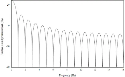
Figure 3: Spectrum of the electrical signal of the low frequency click ...17

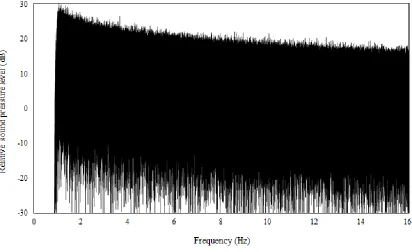
Figure 4: Spectrum of the electrical signal of the pink noise high-pass filtered at 1 kHz .19

Figure 5: Spectrum of the electrical signal of the standard 100 µs click ...20

Figure 6: Diagram depicting the experimental protocol of the ABR condition ...22

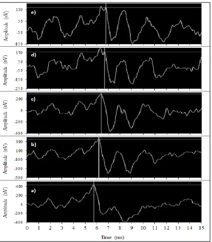
Figure 7: Effect of increasing level of high-pass filtered pink noise on wave V latency ..24

Figure 8: Mean EFR amplitudes across vowel stimuli for the F1 band ...32

Figure 9: Mean EFR amplitudes across vowel stimuli for the F2+ band ...34

Figure 10: Comparison of EFR amplitude differences between polarities for /u/ with and

without h1 in the F1 band ...35

Figure 11: Comparison of EFR amplitude differences between polarities for /a/ with and

Figure 12: Comparison of EFR amplitude differences between polarities for /i/ with and

Figure 13: Histogram of EFR amplitude differences between polarities across vowels in

the F2+ band ...38

Figure 14: Correlation of EFR amplitude differences between polarities for the vowels /i/

(7)

vii

Figure 15: Correlation of EFR amplitude differences between polarities for the vowels /a/

and /u/ in the F1 band...41

Figure 16: Correlation of EFR amplitude differences between polarities for the vowels /a/ and /i/ in the F1 band ...42

Figure 17: Correlation of EFR amplitude differences between polarities for the vowels /u/ and /i/ in the F2+ band ...43

Figure 18: Mean ABR latencies across waves ...45

Figure 19: Mean ABR amplitudes across waves ...46

Figure 20: Histogram of ABR latency differences between polarities across waves ...47

Figure 21: Histogram of ABR amplitude differences between polarities across waves ....48

Figure 22: Correlation of median absolute differences in ABR latency and EFR amplitude in F1 carrier vowels without h1 ...50

(8)

viii

List of Appendices

Appendix A: Ethics approval notice ...66

Appendix B: Sample letter of information and consent...68

(9)

ix

List of Abbreviations

µs Microseconds

A1 Electrode site on the left earlobe

ABR Auditory brainstem response

C Condensation phase

Cz Electrode site on the vertex

dB Decibel

EEG Electroencephalography

EFR Envelope following response

f0 Fundamental frequency

F1 First formant

F2 Second formant

F2+ Region of the second formant and above

FDR False discovery rate

FFR Frequency following response

h1 First harmonic, same frequency as f0

HL Hearing level

Hz Hertz

kHz Kilohertz

(10)

x

MEG Magnetic encephalography

min Minutes

ms Milliseconds

nHL Normal hearing level

nV Nanovolt

p.-p.e. Peak-to-peak equivalent

R Rarefaction phase

RM-ANOVA Repeated measures analysis of variance

s Seconds

SD Standard deviation

SL Sensation level

(11)

Chapter 1

1

Introduction

1.1 Objective aided validation measures

Hearing loss is one of the most common congenital disorders, affecting over 1,100

infants born in Canada every year (Hyde, 2005). Newborn hearing screening programs

have been implemented in many countries across the world to identify hearing loss early

in life, as research has shown that an undetected hearing impairment can have detrimental

long-term effects on cognitive and language development (Hyde, 2005; Joint Committee

on Infant Hearing & American Academy of Pediatrics, 2007). In Ontario, the majority of

newborns are screened within their first month of life and referred to an audiologist for a

full hearing assessment in the case of an abnormal result (Speech-Language & Audiology

Canada, 2010). One frequently used component of the hearing assessment is an

electrophysiological measurement known as the auditory brainstem response (ABR),

which involves presenting a series of click or tone burst stimuli at various rates and

intensities to the child and evaluating if a reliable neural response is present via

electrodes placed on the scalp (Joint Committee on Infant Hearing & American Academy

of Pediatrics, 2007). Information from this test can provide the clinician with the best

estimate of the child’s pure-tone hearing thresholds and, if amplification is the

recommended intervention, may be used to develop prescriptive targets for hearing aids

by the time the child is six months old.

However, a gap exists between the time the child is fitted with hearing aids and the time

the prescribed gain and output level can be confidently validated. In the meantime, it is

possible that certain acoustic features of speech (eg. the fricatives /s/, /z/ or /əz/ at the end

of words to designate plurality) could be missed if they are not amplified to an adequate

level. While audiometric and speech testing are typically employed to validate hearing

aids in adults, these methods are inappropriate for young children who are unable to

produce a reliable behavioural response. In their place, subjective methods such as the

(12)

based on observation in clinical and everyday listening environments for the first two

years (Bagatto et al., 2011). Though this is an effective and validated tool, it requires

several months of observation before conclusions can be drawn about the appropriateness

of the hearing aid output. For this reason, it would be beneficial to have an objective

electrophysiological tool that could provide information about device effectiveness soon

after they have been fitted. This data would nicely augment that collected from the LEAQ

and allow the clinician to ensure the child is getting the best intervention as quickly as

possible.

Ideally, natural speech stimuli should be used to evoke a neural response as it would yield

a better indication of hearing aid performance in everyday listening conditions.

Signal-processing algorithms in the device circuitry are designed to enhance speech while

providing less gain to non-speech sounds; therefore, they may not run in their normal

mode if other types of stimuli are used (Scollie & Seewald, 2002; Easwar, Purcell, &

Scollie, 2012). Unfortunately, using artificial stimuli such as clicks, tone bursts and

modulated tones or noise is more practical as they are steady and will generally elicit a

response that is easier to analyse (Choi, Purcell, Coyne, & Aiken, 2013). This is because,

despite a considerable degree of neural synchronization in response to an auditory

stimulus, the magnitude of the EFR signal is negligible compared to that of the

accompanying myogenic and electroencephalographic noise; thus, many sweeps evoked

by an identical, fixed stimulus must be averaged to attenuate the noise and improve

detection (Jewett & Williston, 1971). Unlike artificial stimuli, natural speech—even

individual phonemes—vary in level, frequency, bandwidth and spectral shape over time

and therefore must often be modified in order to obtain a synchronized neural response in

a reasonable recording time (Scollie & Seeward, 2002; Choi et al., 2013).

The envelope following response (EFR), a steady-state measure that can be evoked by

modified speech stimuli, is of particular interest as a clinical validation measure. The

EFR arises from neurons phase-locked to the stimulus amplitude envelope and can be

elicited by an amplitude modulated tone or a voice’s fundamental frequency (f0) when

producing vowel sounds (Aiken & Picton, 2006; see the “neural generators of the ABR

(13)

advantageous because it can be evoked by running speech stimuli with similar acoustic

characteristics to normal, conversational speech (Aiken & Picton 2006; Choi et al., 2013).

Additionally, the EFR is an objective measure of temporal acuity, the perceptual ability

to discriminate changes in frequency, rhythm and amplitude at suprathreshold levels,

which is crucial for speech comprehension (Purcell, John, Schneider, & Picton, 2004).

For these reasons, the EFR provides an ecologically valid measure of how hearing aids

contribute to natural speech processing, though it has yet to play a significant role in

standardized clinical practice.

1.2 The effect of stimulus polarity on the EFR

In addition to collecting a large number of neural responses to the same stimulus and

averaging across them to attenuate noise, signal detection is routinely improved by

recording responses evoked by opposing polarity stimuli. In the EFR protocol, the

original stimulus waveform (in polarity A) is multiplied by the factor -1 to produce the

opposite polarity waveform (polarity B); the responses are then averaged post hoc (the ‘+ –’ average, see Aiken & Picton, 2008). This protocol is based on evidence that certain

components concomitant with the EFR are highly sensitive to an inversion of stimulus

polarity, and thus contamination from these sources can be reduced (Small & Stapells,

2004, 2005; Aiken & Picton, 2008). These sources include the spectral frequency

following response (FFR), a steady-state response phase-locked to the stimulus fine

structure, the cochlear microphonic, a potential generated by outer hair cells that mirrors

the waveform of the stimulus, and stimulus artifact (Small & Stapells, 2004; Aiken &

Picton, 2008). Meanwhile, the EFR signal is enhanced as the stimulus envelope is

generally unaffected by an inversion of polarity (Krishnan, 2002; Small & Stapells, 2004;

Aiken & Picton, 2008). Though polarity-sensitive differences in EFR amplitude have

been noted in a few studies, these differences tend to be small or non-significant when

averaged across participants (Small & Stapells, 2005; Aiken & Purcell, 2013; Krishnan,

2002).

However, despite studies showing only negligible differences at a group level, there is a

notable degree of individual variation across adult listeners as stimulus polarity is varied.

(14)

fully cancelled when response waveforms to opposite polarities were subtracted and that

this residual EFR varied across the three participants and vowel stimuli (Greenberg,

1980, chapter 7). In a more recent study, Aiken and Purcell (2013) further investigated

the polarity sensitivity of the EFR by analyzing the responses evoked by the f0 of natural

vowel tokens /i/ and /a/. Each vowel token was presented twice in the original polarity

and a third time in the inverted polarity. Absolute values of response amplitude change

across conditions were analyzed for each subject, revealing that the magnitude of change

was significantly greater across opposite polarity conditions than across repeated

measures of the same polarity. Similar to Greenberg’s study, the effect of polarity varied

considerably across participants and vowel tokens, with amplitude changes ranging from

near zero to a maximum of 72 nV (Aiken & Purcell, 2013). Yet, when response

amplitude changes were averaged across the nine participants, the data showed that the ‘+ –’ average was not significantly different from the average across repeated measures of

the same polarity. These findings were further demonstrated in Easwar et al. (2015),

where nearly 30% of the 24 normal hearing participants who had a significant EFR

detection to the stimulus /hεd/ exhibited polarity-sensitive amplitude differences greater

than 39 nV, including one participant who exhibited a difference of 100 nV. Since

test-retest variation in EFR amplitude and fluctuations in electrophysiological noise could

only logically explain differences up to 39 nV, the magnitude of the differences observed

in these subjects indicated a polarity effect (Easwar et al., 2015). However, because the

magnitude and direction of change varied from person to person (e.g., some subjects

exhibited a larger amplitude in response to polarity A than polarity B, whereas others had

the opposite response), the effect of polarity became non-significant when the responses

were averaged across the group.

Though at a group level it may be sufficient to conclude that polarity has only a minor

effect on EFR amplitude, the large degree of polarity-sensitive differences across

individuals has clinical implications if the method is to be adopted into the validation

regimen for hearing aid fittings. Of the 24 participants who had a significant EFR

detection in Easwar et al. (2015), 11 had the significant response in either polarity A or

B, but not both. Furthermore, two participants who exhibited a response in one of the

(15)

individuals who are particularly sensitive to shifts in stimulus polarity, averaging

responses in accordance with the recommended protocol may attenuate response

amplitudes and possibly lead to false negative results (Easwar et al., 2015). Though the

simple solution would be to conduct multiple trials of the EFR in both polarity

conditions, this is not necessarily feasible in a clinical setting due to time constraints,

particularly when testing young children.

An underlying factor that may be contributing to the polarity sensitivity of the EFR is the

degree of envelope asymmetry in speech stimuli. The aforementioned EFR protocol was

originally developed using modulated tone stimuli, which have symmetrical envelopes

around the baseline (Aiken & Picton, 2008). Therefore, though the fine structure would

be inverted in the opposite polarity waveforms, the envelopes would theoretically remain

unchanged and elicit the same neural response. Unfortunately, in the case of natural

speech stimuli, the voice’s first harmonic (h1; same frequency as f0) and other factors

tend to produce varying degrees of envelope asymmetry that may attenuate response

amplitude in the ‘+ –’ average (Skoe & Kraus, 2010; Easwar et al., 2015). Additionally,

h1 may elicit a polarity-sensitive FFR close enough in frequency to the f0 that it could

interfere with the EFR, although studies suggest that this effect is likely minor (Aiken &

Picton, 2006; Aiken & Picton, 2008; Easwar et al., 2015). To account for this potential

confound, Easwar et al. (2015) developed a second experiment that investigated the effect

of h1 on the polarity-sensitive variability of EFR amplitude. Each vowel of the stimulus

/susaʃi/ was high-pass filtered at 150 Hz to remove h1, minimizing envelope asymmetry

and eliminating any contribution from the h1 FFR. Responses elicited by this stimulus in

both polarities were then compared to those elicited by the same stimulus with h1 present

in 20 normal hearing adults. Though results showed that 64.5% of response amplitude

variation due to polarity could be explained by envelope asymmetry, the remaining

variation suggests that there are other factors contributing to the individual differences in

EFR amplitude. Easwar et al. (2015) speculated that this polarity-sensitive variation not

related to envelope asymmetry was most likely arising at some point in the peripheral

(16)

In addition to removing h1, Easwar et al. (2015) made another modification to the /susaʃi/

stimulus that allowed them to simultaneously record EFRs from two separate frequency

bands: one from the region of the first formant (F1) where the harmonics are lower in

frequency and spectrally resolved in the cochlea and the other from the region of the

second formant and above (F2+) where the harmonics are higher in frequency and

spectrally unresolved. The purpose of this modification was to investigate whether the

frequency of the carrier and the type of harmonics in the stimulus influenced the variation

in EFR amplitude. Results from the experiment showed that significant amplitude

differences within participants due to polarity were more commonly found in EFRs

evoked by the F1 carrier, even when h1 (which was only present in the F1 carrier) was

removed. Therefore, it would appear that lower frequency stimuli tend to elicit larger

polarity effects.

1.3 The effect of stimulus polarity on the ABR

The ABR is another evoked response generated in the vestibulocochlear nerve and

brainstem in response to a transient stimulus, such as a click or brief tone burst. The

responses from different parts of this track add together to form a characteristic

waveform with five peaks labeled I to V (see “Neural generators of the ABR and EFR”

section for more detail). Even minute latency differences in waves I, III and V can

indicate cochlear pathology, auditory neuropathy or the presence of an acoustic neuroma

(Schwartz et al. 1990). Similar to EFR protocol, ABR stimuli are often presented in

opposing polarities in an alternating fashion so that polarity-sensitive contaminants such

as the cochlear microphonic and stimulus artifact may be attenuated, though ABR click

stimuli differ in that they are a transient pulse of either rarefied or condensed pressure.

Many researchers have investigated the effect of stimulus polarity on wave latencies and

amplitudes, yielding widely inconsistent results. For example, regarding the latency of

wave V, studies have found shorter latencies to rarefaction phase (R) than condensation

phase (C) stimuli (Ornitz & Walter, 1975; Borg & Lofqvist, 1981; Maurer, Schäfer, &

Leitner, 1980); shorter latencies to C than R stimuli (Pijl, 1987; Hughes, Fino, & Gagnon,

1981); and others have revealed no significant latency differences at all (Kumar, Bhat,

(17)

Beattie & Boyd, 1984; Tietze & Pantev, 1986). In a comprehensive study by Swartz et al.

(1990), 92 participants with normal hearing and 78 participants with mild to severe

cochlear hearing loss (N = 340 ears) were tested with the click-evoked ABR in order to

better quantify the individual variation observed in previous studies. Corresponding with

the results of Rosenhamer et al. (1978), Beattie and Boyd (1984) and others, there were

no significant R-C latency differences when the data was averaged across all participant

ears. However, when absolute R-C latency differences were examined—arguably a more

appropriate method for assessing clinical significance since the magnitude of individual

differences are not obscured by measures of central tendency—there was a surprising

degree of variation. Setting the criterion for a clinically significant R-C latency difference

at ±0.15 ms, a more conservative cutoff value than used in other studies (Borg &

Lofqvist, 1982; Tietze & Pantev, 1986; Beattie, 1988; Edwards, Buchwald, Tanguay, &

Schwafel, 1982), they found that 41%, 46%, and 29% of participant ears exhibited

clinically significant R-C latency differences in waves I, III, and V, respectively.

Furthermore, 27% of participant ears exhibited wave III latency differences as large as

±0.30 ms. Interestingly, though the majority of participants who exhibited this differential

response tended to have shorter wave I and V latencies to clicks presented in R phase,

12% and 7% of participants exhibited the opposite response, with shorter latencies to

clicks presented in C phase. This finding has been replicated in many studies

(Schoonhoven, 1992; Borg & Lofqvist, 1982; Orlando & Folsom, 1995; Coats & Martin,

1977) and is remarkably similar to the variation found in EFR studies. Cats and gerbils

also exhibit a substantial degree of individual variability in response to varying stimulus

polarity (Tvete & Haugsten, 1981; Burkard & Voigt, 1989). Furthermore, when Stockard,

Stockard, Westmoreland and Corfits (1979) and Orlando and Folsom (1995) tested a few

of their subjects with the most distinctive responses six months later, they exhibited the

same latency patterns, indicating that the majority of the individual variation is

originating from physiologic factors and remains relatively stable over time.

(18)

clicks increased in four of the five cats (Tvete & Haugsten, 1981). Stockard et al. (1979) also found that latency differences are minimal at lower stimulus levels (30 and 40 dB SL) and greater at higher levels (50 to 70 dB SL). However, when Beattie (1988) varied the click level between 60, 75 and 90 dB nHL and Orlando and Folsom (1995) varied the level of single-cycle sinusoids between 40 and 60 dB nHL, neither study found a

consistent trend of variation related to stimulus intensity in normal hearing adults. Ballanchanda, Moushegian and Stillman (1992) also failed to find a significant effect of intensity on latency in regards to polarity differences, though they did find a small effect on peak amplitudes. Looking at responses from the auditory nerve recorded from the round window of the cochlea, Peake and Kiang (1962) found the most striking polarity differences in latency and morphology at moderate stimulus intensities. A study by Rawool and Zerlin (1988) found that when click level was increased from 35 to 95 dB SPL in 10 dB steps, all six participants exhibited a shift from shorter latencies to C clicks to shorter latencies to R clicks, though the level at which this occurred varied

considerably. Orlando and Folsom (1995) also saw this shift in their data, but with more variability—some participants exhibited shorter latencies to R stimuli at low levels and longer latencies at high levels, whereas others showed the opposite response or exhibited no change at all. In summary, individual variability to stimulus polarity makes it difficult to identify a consistent trend of intensity, though in general it would appear that variation is greatest when stimuli are presented at moderate to high intensities (50 or 60 dB nHL and higher).

(19)

effect of stimulus frequency on polarity-sensitive ABR variation was further confirmed by Schoonhoven (1992) in a derived band paradigm, where alternating polarity clicks were presented with high-pass noise at various cut-off frequencies. Results showed that the greatest differences in wave III and V latency due to polarity occurred when the cutoff frequency was 1.6 kHz and lower (Schoonhoven, 1992). Other studies demonstrating this effect include Salt and Thornton (1984) and Coats (1978).

Interestingly, these results correspond closely with the findings from the Easwar et al. (2015) EFR study, where the degree of polarity-sensitive variation was larger when elicited by the lower frequency carrier.

The effect of low frequency energy in the stimulus on polarity-sensitive variation may be one of the underlying factors explaining why those with high frequency hearing loss tend to show even greater R-C latency differences than those with normal hearing. In their large subset of hearing impaired participants, Schwartz et al. (1990) found a clear trend of greater R-C latency differences in waves I, III and V as the average degree of high

frequency hearing pure tone sensitivity loss at 2000, 3000 and 4000 Hz increased. Borg and Lofqvist (1982) also found greater wave V R-C latency differences in 29 ears with steep high frequency hearing loss, whereas Coats and Martin (1977) only found

significant differences in waves II to IV. Polarity-sensitive variation also appears to be greater in those with diseases affecting the brainstem and auditory nerve, such as multiple sclerosis and acoustic neuromas (Maurer, 1985; Emerson, Brooks, Parker, & Chiappa, 1982).

To an extent, the increased polarity sensitivity elicited by lower frequency stimuli can be explained physiologically. In the simplest model, the initial phase of a R stimulus causes the diaphragm of an earphone to move inwards, creating a wave of rarefied pressure that propagates down the ear canal and induces an outward movement of the tympanic

(20)

1994). In the case of C stimuli, the diaphragm of the earphone moves outwards leading to deflection of the basilar membrane towards the scala tympani and displacement of the inner hair cells away from the stria vascularis, thereby hyperpolarizing the cells and inhibiting neural firing of the auditory nerve (Peake & Kiang, 1962; Møller, 1994). After a half-cycle delay, the excitatory phase following the initial C peak depolarizes the sensory cells and increases auditory nerve firing; therefore, if the neural response to the stimulus is being measured at the brainstem, C waves should theoretically lag behind R waves by this half-cycle period (Peake & Kiang, 1962; Don, Vermiglio, Ponton, Eggermont, & Masuda, 1996). In a high frequency stimulus, the half-cycle is almost negligible; however, the half-cycle of a low frequency stimulus (eg. 1 ms for a 500 Hz stimulus) is considerably longer and should have a notable effect on wave latencies (Don et al., 1996). However, a review of ABR latency data would suggest that this model is too simplistic—not only do latency differences frequently deviate from the expected half-cycle delay, but many individuals actually exhibit shorter wave latencies to C than to R stimuli, as previously mentioned. Experiments conducted on cats and chinchillas have found that, depending on the stimulus frequency and intensity, hair cells can become excited by basilar membrane deflection in both directions and so are capable of

depolarizing to an initial peak of either phase (Sokolich, 1980; Ruggero & Rich, 1983; Antoli-Candela & Kiang, 1978; Kiang, Watanabe, Thomas, & Clark, 1965). Additionally, fluid velocity and tectorial membrane displacement appear to interact with hair cell depolarization in a complex manner that is poorly understood (Ruggero & Rich, 1983).

(21)

Don et al., 1996). Alternatively, phase-locking neurons throughout the brainstem may also show a pattern of excitation and synchronization unique to the individual (Debruyne, 1994).

1.4 Neural generators of the ABR and EFR

The similarities between the polarity-sensitive variation seen in the EFR and ABR suggest that the variation could arise from a common source (or sources). Therefore, it may be helpful to compare what is known about the neural generators of the ABR and EFR (see Figure 1 for diagram of brainstem anatomy). The ABR is generated by neurons throughout the brainstem and peripheral auditory system that are evoked by the onset of a transient stimulus, such as a click or brief tone burst. The recorded response takes the shape of a characteristic waveform with a series of normative peaks representing

synchronized responses from sequential sites in the neural pathway (Jewett & Williston, 1971). The earliest components of the waveform, waves I and II, are generated by the distal and proximal portions of the vestibulocochlear nerve, respectively (Møller,

Jannetta, & Møller, 1981; Møller, Jannetta, & Sekhar, 1988; Møller, 1994). At this point, the ascending auditory system diverges into several parallel pathways, making it difficult to pinpoint the exact structures in the brainstem that are generating the next three waves. Intracranial studies suggest that wave III is generated primarily by the cochlear nucleus (Møller & Jannetta, 1982; Møller, 1994), wave IV by third-order neurons in the superior olivary complex (Møller & Jannetta, 1982; Møller, 1994), and wave V by the termination of the lateral lemniscus on the contralateral side of the inferior colliculus (Møller & Jannetta, 1982; Møller, 1994). However, these studies also show that waves III, IV, and V are highly complex and likely have contributions from more than one brainstem structure (Møller, 1994).

(22)

Figure 1: Diagram of the brainstem showing the locations of the main nuclei and

fibre tracks of the ascending auditory system.

Cochlear nucleus (CN), superior olivary complex (SOC), lateral lemniscus (LL),

(23)

the cortex with an approximate latency of 29 ms (Frisina, 2001; Herdman et al., 2002; Kuwada et al., 2002; Purcell et al., 2004). It is generally accepted in the literature that cortical sources of envelope following responses respond best to lower modulation rates (< 50 Hz), whereas subcortical components contribute a growing amount as modulation rate increases (Herdman et al., 2002; Kuwada et al., 2002; Purcell et al., 2004), though new evidence has emerged suggesting that the human auditory cortex contributes more at higher modulation rates than previously thought (Coffey, Herholz, Chepesiuk, Baillet, & Zatorre, 2016). In the case of speech stimuli where harmonics are amplitude modulated at the f0 (between 88 Hz and 100 Hz in this present study), the neural response contains

large contributions from subcortical structures (Herdman et al., 2002; Aiken & Picton, 2006). Intracellular recordings in rabbits and gerbils have identified peak amplitude responses at the level of the cochlear nucleus and inferior colliculus at frequencies comparable to the f0 of speech (Frisina, Smith, & Chamberlain, 1990; Kuwada et al.,

2002). Coffey et al. (2016) also identified the cochlear nucleus and inferior colliculus, as well as the medial geniculate and auditory cortex, as dominant generators when using MEG to record responses to the speech stimulus /da/ in 22 young adults.

1.5 Purpose of this thesis

(24)

Chapter 2

2

Methods

2.1 Participants

Thirty-one adults (26 females, 5 males) between the ages of 22 and 34 (mean age 24.8

years; standard deviation 2.88 years) were recruited from the Western University

community in London, Ontario to participate in the study. All participants reported

English as their first language and reported no hearing, speech, language or neurological

impairments. Using a 10 dB-down, 5 dB-up bracketing technique, audiometric thresholds

were obtained at octave and inter-octave frequencies between 250 and 4000 Hz with a

Madsen Itera audiometer and TDH-39 headphones. The upper testing level of 4000 Hz

was chosen because vowels have most of their energy below 4000 Hz. All participants

had thresholds below 20 dB HL across test frequencies. Routine otoscopy revealed no

occluding wax, discharge, or foreign objects that may have negatively impacted results.

Participants provided informed consent and were compensated for their time. The study

was approved by the Health Sciences Research Ethics Board of Western University.

2.2 Stimuli

EFRs were evoked by the vowels /u/ (as in ‘hoot’), /a/ (as in ‘pot’) and /i/ (as in ‘heat’) in

the stimulus token /susaʃi/, previously developed and used by Easwar et al. (2015). The

vowels, representing a range of F1 and F2 frequencies, were produced by a 42 year old

male talker from Southwestern Ontario and were individually edited using the software

Praat (Boersma, 2001)to elicit two separate EFRs—one arising from the lower frequency

F1 region and the other from the higher frequency F2+ region (see Easwar et al., 2015 for

more detail). In brief, the F1 and F2+ bands were isolated by filtering each vowel at a

cutoff frequency approximating the midpoint between F1 and F2. The f0 of the F1 band

was then lowered by 8 Hz and recombined with the F2+ band to form dual-f0 vowels.

Once reassembled as /susaʃi/, the stimulus waveform (in polarity A) was multiplied by

the factor -1 to produce the opposite polarity waveform (polarity B). It should be noted

that both polarity waveforms produce both rarefied and condensed pressure, as they

(25)

An additional modification was made to a copy of the dual-f0 /susaʃi/ stimulus in each

polarity to account for the influence of stimulus envelope asymmetry on EFR polarity

sensitivity. Easwar et al. (2015) high-pass filtered each vowel at 150 Hz in Praat in order

to remove the first harmonic, h1, from the F1 band, significantly reducing the envelope

asymmetry of each vowel. A pilot study of 8 participants established that the vowel

category was perceived to be the same after the removal of h1. The modified stimulus

token was then concatenated with the original dual-f0 token of the same polarity.

Therefore, the full EFR stimulus sequence comprised four tokens of /susaʃi/: two were

presented in polarity A with and without h1, then two were presented in polarity B with

and without h1. Each sweep was 8.2 s and was presented 300 times for a total duration of

41 min. See Figure 2 for the amplitude-time waveform of the /susaʃi/ stimulus.

ABRs were evoked by a series of stimuli developed in Praat. Using the ‘Create new

sound from formula’ function, a 1 ms R click (formula = -0.05) was created and

concatenated with 20 ms of preceding silence and 54 ms of following silence (formula =

0) to produce a single 75 ms R click stimulus at a sampling rate of 32000 Hz. This

stimulus was then copied and strung together many times to produce a train of 2000 R

clicks with a total duration of 150 s and a presentation rate of 13.3 clicks per second. This

relatively slow presentation rate was chosen to obtain the clearest ABR waveforms

possible. A second click train of the same duration and presentation rate was made with

clicks alternating between R and C phase. A single 75 ms C click was created in the same

fashion as the R click, but with a positive rather than a negative amplitude (formula =

0.05). Beginning with the R stimulus, the stimuli were then concatenated many times

until an alternating click train of 1000 clicks of each polarity was obtained. Longer in

duration than the standard 100 µs click stimulus used in clinical practice, these R and C

click stimuli contained significant acoustic energy around 300 Hz with a null at 1 kHz.

The decision to use a click stimulus with a greater proportion of low frequency energy

was based on evidence in the ABR literature suggesting that lower frequency stimuli

elicit greater polarity differences (Coats, 1978; Gorga, Kaminski, & Beauchaine, 1991;

Orlando & Folsom, 1995; Salt & Thornton, 1984; Schoonhoven, 1992). See Figure 3 for

(26)

Figure 2: Amplitude-time waveform of /susaʃi/ stimulus.

Though the F1 and F2+ carriers are illustrated separately here, they are presented

(27)

(28)

The click trains were also presented with ipsilateral masking noise to ensure that the

ABRs were generated from the low frequency apical region of the cochlea and not the

high frequency base through spread of the traveling wave. Using the ‘Create new sound

from formula’ function in Praat, 720 s of white noise (formula = randomGauss [0,0.1])

was created at a sampling rate of 32000 Hz, then modified into pink noise which contains

equal energy in each octave (formula = if x > 100 then self*sqrt[100/x] else 0 fi, with x

representing frequency). This stimulus, henceforth referred to as full band pink noise,

was used during the preparation phase of the ABR condition to determine the minimum

level of masking noise required to generate an ABR from the apical region of the cochlea.

A copy of the full band pink noise stimulus was high-pass filtered at the cutoff frequency

1 kHz (see Figure 4). This stimulus, henceforth referred to as high-pass filtered pink

noise, was used during the data collection phase of the ABR condition. Both the

high-pass filtered and full band pink noise stimuli were trimmed to 150 s, the same duration as

the R and alternating polarity click trains.

To evoke a standard ABR for comparison, a final 150 s click train with classic 100 µs

clicks was developed. Similar to the creation of the low frequency click train, 100 µs

clicks (R = -0.05; C = 0.05) were created in Praat and concatenated with 20 ms and 54.9

ms of silence to produce individual 75 ms click stimuli, then strung together into a train

of 2000 alternating polarity clicks beginning with R phase. These standard clicks had a

flat acoustic spectrum to about 6 kHz, after which acoustic energy began to decline (see

Figure 5).

2.3 Stimulus presentation

Stimulus presentation and data acquisition were controlled by software developed using

LabVIEW (version 8.5; National Instruments, Austin, TX, USA). A National Instruments

PCI-6289 M-series acquisition card was used to convert the stimuli from digital data to

analog signals, as well as to convert the EEG input from analog to digital. All stimuli

were presented at a 32000 Hz sample rate with 16-bit resolution, with EFRs recorded at

8000 samples per second and ABRs recorded at 32000 samples per second with 18-bit

resolution. Stimuli levels were controlled by a Tucker-Davis Technologies PA5

(29)

Figure 4: Spectrum of the electrical signal of the pink noise high-pass filtered at

1 kHz.

Due to physical characteristics of the Etymotic ER-2 stimulus transducer, the relative

sound pressure level of the acoustic spectrum decreased more rapidly with frequency

(30)

Figure 5: Spectrum of the electrical signal of the standard 100 µs click.

Due to physical characteristics of the Etymotic ER-2 stimulus transducer, the relative

sound pressure level of the acoustic spectrum decreased more rapidly with frequency

above 10 kHz. There was a pressure node closer to 11 kHz than exactly 10 kHz due to

(31)

The order of the EFR and ABR conditions was counterbalanced. Though the majority of

participants completed both conditions in a single session, three participants chose to

complete the EFR and ABR in two separate sessions within a week apart.

2.3.1 EFR condition

In the EFR condition, the /susaʃi/ stimulus was presented at 65 dB SPL for 300 sweeps,

which required 41 min. Stimulus level was calibrated using a Brüel and Kjær Type 2250

sound level meter in flat-weighted Leq mode as the stimulus played for 60 s into a Type

4157 ear simulator.

2.3.2 ABR condition

The ABR condition required multiple measurements that were shorter in duration than

the EFR condition (see Figure 6 for a diagram of the condition’s experimental protocol).

First, 2000 of the low frequency (1 ms in duration) clicks in R phase were presented at 95

dB peak-to-peak equivalent (p.-p.e.) SPL to obtain a baseline ABR waveform. This level

was calibrated using the sound level meter in flat-weighted mode and observing the

waveforms on an oscilloscope where the peak-to-peak amplitude of a 300 Hz tone was

matched to the stimulus waveform. This level also corresponded to 59 dB nHL,

established by obtaining the minimum average hearing threshold for each of the ABR

click stimuli from nine normal hearing adults prior to the study.

2.3.2.1 ABR preparation phase

Once the baseline ABR waveform was obtained, the next objective was to find the

minimum level of ipsilateral masking noise needed to ensure that the apical region of the

cochlea was generating the ABR. This was accomplished in a two-step preparation phase.

First, the minimum level of full band pink noise required to eliminate wave V in the ABR

was found. During successive presentations of 2000 low frequency R clicks, the level of

full band pink noise was varied in 5 dB steps between 43 and 53 dB nHL (68 and 78 dB

SPL; calibrated in slow flat-weighted mode) depending on the individual. On average, the

minimum level of pink noise needed to significantly attenuate wave V was 50 dB nHL

(32)

(33)

frequency R clicks to confirm that the minimum noise level determined in the previous

step would adequately shift the latency of wave V. A low frequency ABR should have a

1 to 2 ms shift in wave V latency from the baseline waveform, as it takes longer for

mechanical energy introduced by the stapes at the cochlear window to reach the apical

region of the cochlea than the basal region (Don & Eggermont, 1978; Burkard & Hecox,

1983). Figure 7 illustrates the shift in wave V latency in one participant with increasing

level of high-pass filtered pink noise.

2.3.2.2 ABR data collection phase

Next was the data collection phase, where the ABRs for use in the analysis were

recorded. A run of 4000 low frequency alternating polarity clicks was presented at 95 dB

p.-p.e. SPL (59 dB nHL) with the previously selected level of high-pass filtered pink

noise. Though the actual click train stimulus was only 2000 clicks and 150 s in duration,

the LabVIEW program seamlessly repeated the click train and pink noise so that the

responses to 2000 clicks of each polarity could be obtained in a single run. The

measurement was repeated another two times for a total of three runs of 4000 low

frequency alternating clicks. The last step of the ABR condition was to record three runs

of 4000 standard (100 µs in duration) alternating polarity clicks for comparison. The

clicks were presented at 93 dB p.-p.e. SPL (55 dB nHL) without ipsilateral masking

noise. The total duration of the ABR condition ranged from 45 to 50 min.

2.4 Response recording

To record the EEG, four disposable Medi-Trace Ag/AgCl electrodes were applied to the

skin using Grass Technologies EC2 electrode cream. The inverting electrode for the EFR

was placed on the posterior midline of the neck below the hairline, whereas the inverting

electrode for the ABR was placed on the left earlobe (A1). The last two electrodes were

placed on the vertex (Cz) and collarbone and acted as the non-inverting and ground

electrodes, respectively, for both the EFR and ABR. Each electrode site was gently

cleaned with NuPrep skin gel and an alcohol wipe to ensure that all electrode impedances

were less than 5 kΩ and within 2 kΩ of each other, as measured with an F-EZM5 Grass

(34)

Figure 7: Effect of increasing level of high-pass filtered pink noise on wave V

latency.

ABR waveforms from one participant evoked by low frequency clicks with varying

levels of high-pass filtered noise. Wave V is marked with a crosshair cursor in each

panel. a) No noise, b) noise level at 28 dB nHL (53 dB SPL), c) noise level at 38 dB

nHL (63 dB SPL), d) noise level at 48 dB nHL (73 dB SPL), e) noise level at 53 dB

(35)

After electrode placement, participants were seated in an electromagnetically shielded

sound booth and reclined into a relaxed position, with a blanket provided for comfort. A

rolled towel was placed behind their neck to support the head and reduce muscle artifact.

An Etymotic ER-2 mu-metal shielded insert earphone (shielded by Intelligent Hearing

Systems) with an appropriately sized foam tip was placed into the left ear canal. For the

EFR condition, the non-inverting, ground, and posterior neck inverting electrode

recording leads were plugged into a Grass LP511 EEG amplifier set to bandpass filter

between 3 and 3000 Hz. For the ABR condition, the posterior neck inverting electrode

lead was switched out for the earlobe inverting electrode lead and the lower filter setting

of the amplifier was changed to 100 Hz. In both conditions, the amplifier applied a gain

of 50000 to the input EEG, which was further increased by two to 100000 by the

PCI-6289 card. Electrode recording leads were carefully separated from the ER-2 transducer

to reduce stimulus artifact. Lastly, the booth lights were switched off and participants

were encouraged to close their eyes and sleep in order to minimize muscle noise.

2.5 Response analysis and detection

Though the EEG waveforms and spectra were displayed during EFR and ABR data

collection, the analysis was conducted offline. EFR analysis was performed using

MATLAB (version 7.11.0 [R2010b]; MathWorks, Natick, MA, USA) in a similar method

as Easwar, et al. (2015). First, each 8.2 s sweep was divided into 8 epochs and a noise

metric of the averaged EEG amplitude between 80 and 120 Hz was calculated. This noise

metric included all muscle and brain activity, including the EFR signal. Any epoch with a

noise metric that exceeded two standard deviations above the mean noise metric was

rejected from the analysis, as it was assumed to be dominated by muscle artifact. Epochs

that passed this noise rejection were used to calculate a synchronous average sweep.

Next, a Fourier analyser was used to compare the average sweep to a reference signal

over time to estimate the EFR. Sine and cosine sinusoids were generated from the

instantaneous f0 frequency to act as the reference signal. After correcting for an estimated

brainstem processing delay of 10 ms as in previous related studies (Aiken & Picton,

2006; Choi et al., 2013; Easwar et al., 2015; Purcell et al., 2004), the EEG was multiplied

(36)

estimate of EFR amplitude and phase was obtained by averaging these components

across the duration of the vowel into a single complex number, then corrected for

possible overestimation from noise (Easwar et al., 2015; Picton, Dimitrijevic,

Perez-Abalo, & Van Roon, 2005). This was repeated for the three vowels with and without h1,

in both F1 and F2+ carriers and in both polarities, for a total of 24 EFR estimates.

In addition to computing the EFR amplitude and phase of a vowel, the Fourier analyser

used six frequency tracks below and eight frequency tracks above the f0 response track to

estimate the background EEG noise. The separation in Hz of the frequency tracks was

different for each vowel as it varied with analyser bandwidth, which is the reciprocal of

the vowel duration. Certain tracks, such as the one containing 60 Hz or those that

overlapped with the other response track (for F1 or F2+), were excluded. The EEG noise

from all 14 frequency tracks was averaged to produce a single noise estimate used in

comparison to the EFR amplitude estimate in an F-test. If the ratio of EFR amplitude to average background noise exceeded the critical F-ratio (2, 28 degrees of freedom) of 1.82 at an α of 0.05, then an EFR was considered to be detected for that condition.

There were many occasions where a participant would exhibit a significant EFR detection

to a vowel stimulus in one polarity, but not the other. Easwar et al. (2015) also noted this

in their experiments, speculating that the discrepancy may be due to an effect of polarity

sensitivity. To account for this potential effect, Easwar et al. (2015) included the

participant’s data for that vowel if a significant detection was found in at least one of the polarity conditions. This ‘either polarity’ rule was based on the assumption that the

response estimate in the polarity condition considered non-significant represented a small

amplitude EFR that could not be statistically distinguished from the noise floor. A

Bonferroni correction (critical p value = 0.025) was applied to increase the stringency of EFR detections and account for multiple comparison bias. Applying this ‘either polarity’

rule increased the number of significant EFR detections in their sample; however, they

still found that a considerable number of subjects had a non-significant EFR detection in

at least one vowel condition (20% of subjects in the F1 band and 30% of subjects in the

(37)

Initially, the present study emulated the methods of Easwar et al. (2015) and employed

the same ‘either polarity’ rule. Unfortunately, an even greater number of subjects were

found to have at least one non-significant EFR detection after the rule had been applied

(26% of subjects in the F1 band and 42% of subjects in the F2+ band). Since all of the

data from these participants would need to be excluded in order to complete the repeated

measures analysis of variance (RM-ANOVA) portion of the analysis, employing the

‘either polarity’ rule was appropriate for this present study, as it would not accurately

represent the true portrait of polarity sensitivity in the population. Instead, all EFR data

was included in the analysis regardless of significant detection. To reduce the impact of

noise on EFR estimates as much as possible while still maintaining a maximum sample

size, the noise estimates computed for each vowel condition in MATLAB were averaged

across all participants and conditions (mean = 28.84 nV, SD = 10.59 nV). EFR data from subjects with noise values that exceeded 2 SDs of the mean (50.01 nV) in over 10% of

conditions were excluded from the analyses (3 subjects), as their values were likely to be

highly influenced by muscle artifact.

ABR analysis was performed using software developed with LabVIEW. Each run was

individually loaded into the program and a noise metric was calculated for the averaged

EEG amplitude between 100 and 500 Hz for each 10-click (0.75 s) epoch. Like in the

EFR analysis, any epoch that exceeded the mean noise metric by two standard deviations

was rejected. Once a run was processed, two waveform traces were displayed on a

separate panel of the LabVIEW program so that responses to odd number clicks were

grouped together into one average waveform and responses to even number clicks into

another. In the case of the run of low frequency R clicks without noise, both of the

resulting traces were average responses to R clicks and therefore were combined into a

grand average waveform. Each run of alternating polarity clicks, however, produced one

trace that was the average response to R clicks and another that was the average response

to C clicks. The three runs of standard alternating polarity clicks were loaded into the

program and the R and C traces were combined into a grand average R waveform and a

grand average C waveform. This process was repeated for the three runs of low

(38)

The latencies and amplitudes of waves I, III, and V were marked by an evaluator on each

of the five grand average waveforms. Latency was marked at the peak for waves I and III,

and on the shoulder for wave V. Amplitude was determined by marking the peak

amplitude and the amplitude of the following valley, then finding the difference.

Unfortunately, masking the low frequency click train with ipsilateral high pass pink

noise, though necessary for obtaining an ABR from the apical region of the cochlea,

inevitably reduced the robustness of the response and attenuated peak amplitudes. As a

result, many of the R and C waveforms became significantly degraded despite using the

minimum noise level. Waveforms that were particularly difficult to interpret were marked

by a second independent evaluator and results were compared; however, in some cases

only wave V could be confidently identified. Two participants with significantly

degraded waveforms returned for an additional three to four runs of the alternating low

frequency click train at lower noise levels. Much less ambiguous, these waveforms were

used for comparison when marking the original R and C grand average waveforms.

Another participant with significantly degraded waveforms was unable to return for

additional ABR measurements and was therefore excluded from all ABR analyses.

2.6 Stimulus artifact checks

To check for stimulus artifacts in the ABR condition which may be caused by

electromagnetic leakage, an individual was fitted with three electrodes in the ABR

montage and situated in the sound booth as usual. Instead of inserting the foam tip of the

transducer into the individual’s ear canal, the tip was placed inside a Zwislocki coupler

(an ear simulator) resting beside the individual. Each stimulus was presented for its full

duration and the responses were analysed offline in the LabVIEW program in the same

fashion as the main experiment. No stimulus artifacts were observed. The total recording

time was 20 min.

To check for stimulus artifacts in the EFR condition, 15 individuals were fitted with three

electrodes in the EFR montage and situated in the sound booth as usual. As in the ABR

artifact check, the /susaʃi/ stimulus was routed to the Zwislocki coupler resting beside the

individual. The total recording time per participant was 41 min. Afterwards, the EFR data

(39)

significant EFR detections found were labeled as false positives. Across the 15

individuals, the false positive rate was 4.4% for polarity A and 6.7% for polarity B. Since

the difference between the two polarity conditions was marginal and close to the

expected α of 0.05 for type I error, it is unlikely that false positives had a significant

impact on the polarity-sensitive amplitude differences observed in the EFR.

2.7 Statistical analyses

EFR and ABR statistical analyses were completed using SPSS (version 24; IBM,

Armonk, NY, USA). Emulating the analysis from Easwar et al. (2015), a three-way

RM-ANOVA was completed with EFR data in the F1 band to compare the effects of polarity

across vowel stimuli. The three within-subject factors were polarity (A or B), vowel (/u/,

/a/ or /i/) and h1 (present or absent). A RM-ANOVA was also completed for EFR data in

the F2+ band, however, because h1 was only present in the F1 band the data set was

collapsed into two levels, polarity and vowel, thereby doubling the sample size to 56.

Significant interactions between within-subject variables, interpreted at an α of 0.05, were analysed post-hoc using Sidak-corrected pairwise comparisons.

To evaluate the effect of polarity on ABR wave latencies and amplitudes, multiple paired

t-tests were completed for waves I, III and V. Results were evaluated using critical p

values determined by the False Discovery Rate (FDR) method (Benjamini & Hochberg,

1995) for multiple comparisons.

Polarity-sensitive differences in EFR data were compared to those found in ABR data

using correlational analyses. Latency and amplitude differences were calculated by

subtracting polarity A from polarity B for the EFR and subtracting C from R for the

ABR. Absolute differences were also calculated. To obtain a more global picture of an

individual’s polarity sensitivity, maximum and median amplitude differences were

identified across F1 carrier vowels with h1, F1 carrier vowels without h1 and all F2+

carrier vowels, as well as latency differences across ABR waves. This approach was

selected to avoid computing correlations for every possible relationship, as there would

be 144 to consider (eg F1 /u/ with h1 amplitude difference vs. wave I latency difference,

(40)

etc.), and to increase the sample size and power of each test. Results were interpreted

(41)

Chapter 3

3

Results

3.1 Effect of polarity on the EFR

A three-way RM-ANOVA was completed to examine the effects of polarity, h1 and

vowel on EFR amplitude in the F1 band. Twenty-eight of the 31 adults who participated

in the study were included in the analysis, as three subjects were removed due to

excessive noise. Prior to the comparison of within-subject effects, a Mauchly’s test for

sphericity was computed for each within-subject factor to determine if the variances of

the differences between all possible pairs of groups were significantly different. The test

indicated that the assumption of sphericity had not been violated for the three-way

interaction of polarity, h1 and vowel, χ2_{(2) = 0.799,}_p_{= 0.671; therefore, it was}

unnecessary to correct the degrees of freedom. The RM-ANOVA revealed a significant

three-way interaction between the effects of polarity, h1 and vowel on EFR amplitude,

F(2, 54) = 3.184, p = 0.049, η2partial = 0.105. Post-hoc tests using the Sidak correction for

multiple comparisons were completed to further investigate this interaction. For the

vowel /u/ with h1, polarity A amplitude (140.11 ± 11.56 nV) was significantly greater

than polarity B amplitude (117.59 ± 8.81 nV) by a mean of 22.52 nV, p = 0.011, 95% CI [5.49, 39.55]. For the vowel /u/ without h1 the trend was reversed: polarity A amplitude

(108.72 ± 9.13 nV) was significantly lower than that of polarity B (138.26 ± 11.01 nV)

by a mean of 29.54 nV, p < 0.001, 95% CI [14.54, 44.54]. The amplitude of polarity A was also significantly greater than that of polarity B for the vowel /a/ with h1 (128.18 ±

11.11 nV and 103.49 ± 9.27 nV, respectively) by a mean of 24.69 nV, p = 0.002, 95% CI [10.10, 39.28]. The mean amplitude difference between polarity A and B approached

significance for the vowel /i/ without h1, p = 0.072. There were no significant differences between polarity conditions for /a/ without h1 and /i/ with h1. EFR amplitude differences

across conditions, as well as the average electrophysiological noise estimate for each are

illustrated in Figure 8.

A two-way RM-ANOVA was conducted to examine the effects of polarity and vowel on

(42)

Figure 8: Mean EFR amplitudes across vowel stimuli for the F1 band.

(43)

analysis were included. Since h1 would have no bearing on EFR amplitudes in the F2+

band, EFRs with and without h1 were combined under each vowel category, thereby

doubling the sample size (N = 56). Mauchly’s tests computed for each within-subject variable indicated that sphericity had not been violated for the main effect of vowel or for

the interaction of polarity and vowel, χ2_{(2) = 1.038,}_p_{= 0.595 and χ}2_{(2) = 1.069,}_p₌

0.586, respectively. Only vowel was found to have a significant main effect on EFR

amplitude, F(2, 110) = 30.04, p < 0.001, η2

partial = 0.35. Pairwise comparisons with Sidak

correction completed post-hoc revealed that the amplitude of /a/ (113.73 ± 4.37 nV) was

significantly greater than that of /u/ (83.71 ± 5.16 nV) by a mean difference of 30.02 nV,

p < 0.001, 95% CI [18.40, 41.65]. The amplitude of /a/ was also significantly greater than that of /i/ (83.38 ± 4.91 nV) by a mean difference of 30.36 nV, p < 0.001, 95% CI [19.12, 41.59]. The amplitudes of /u/ and /i/ were not significantly different from each other. A

main effect of polarity on EFR amplitude approached significance, F(1, 55) = 30.04, p = 0.069, η2partial = 0.059. EFR amplitude differences across conditions in the F2+ carrier are

illustrated in Figure 9.

In agreement with the findings of Easwar et al. (2015), the degree of polarity sensitivity

of EFR amplitude varied considerably across individuals. Histograms were constructed to

compare individual amplitude differences between polarities across vowel, h1 and carrier

conditions. Figures 10 through 13 illustrate the directionality of amplitude changes by

plotting the differences of polarity A amplitude minus polarity B amplitude. Positive

differences indicate a greater amplitude in the polarity A condition than the polarity B

condition, whereas negative differences indicate the reverse. Though the majority of

subjects exhibited small amplitude differences less than 30 nV, seven individuals

exhibited differences greater than 100 nV in at least one condition.

Furthermore, it would appear that, in general, those who exhibit large differences in one

vowel condition tend to have similarly large differences in the other two vowel

conditions as well. Amplitude difference data was grouped into the three vowel

(44)

Figure 9: Mean EFR amplitudes across vowel stimuli for the F2+ band.

(45)

Figure 10: Comparison of EFR amplitude differences between polarities for /u/

with and without h1 in the F1 band.

The vertical dashed line marks the bin containing zero difference in response

(46)

Figure 11: Comparison of EFR amplitude differences between polarities for /a/

(47)

Figure 12: Comparison of EFR amplitude differences between polarities for /i/

(48)

Figure 13: Histogram of EFR amplitude differences between polarities across

vowels in the F2+ band.

(49)

coefficient. A positive, moderate-strength correlation was found between /u/ and /i/ in the

F1 band, indicating that as the degree of polarity sensitivity increased in one vowel it also

increased in the other, r = 0.462, N = 56, p < 0.001, critical p value = 0.008 (see Figure 14). There were also positive correlations between /u/ and /a/ (r = 0.272, N = 56, p = 0.042, critical p value = 0.033) and /a/ and /i/ (r = 0.283, N = 56, p = 0.035, critical p

value = 0.025) in the F1 band, though these relationships were not as strong and failed to

reach significance (see Figures 15 and 16). In the F2+ band, a moderate-strength, inverse

correlation between /u/ and /i/ approached significance, r = -0.307, N = 56, p = 0.021, critical p value = 0.017 (see Figure 17).

It is possible that fluctuations in noise between polarity A and polarity B conditions could

be contributing to EFR amplitude differences. To account for this potential confound,

correlation analyses were completed comparing the absolute differences in noise

estimates to those in EFR amplitude between the polarity conditions. Spearman’s rho was

used to analyse the correlations due to the highly right-skewed nature of the absolute

difference distributions. The correlations indicated no significant relationships between

the variables in the F1 (r = 0.104, N = 168, p = 0.179) and F2+ bands (r = 0.026, N = 168,

p = 0.738). Therefore, as Easwar et al. (2015) also concluded, it is unlikely that variations in noise are significantly contributing to the EFR amplitude differences observed between

polarity conditions.

3.2 Effect of polarity on the ABR

Multiple paired t-tests were completed to examine polarity sensitive differences in the

latency and amplitude of waves I, III and V. Of the 31 participants, 20 had an identifiable

wave I, 23 had an identifiable wave III and 30 had an identifiable wave V in both R and

C conditions. R latency (M = 3.04 ms, SD = 0.68 ms) was found to be significantly longer than C latency (M = 2.71 ms, SD = 0.46 ms) for wave I after FDR correction by a mean difference of 0.33 ms, t(19) = 2.74, p = 0.031, critical p value = 0.033, 95% CI = [0.03, 0.62]. R latency was also numerically longer than C latency for wave V, though this

(50)

Figure 14: Correlation of EFR amplitude differences between polarities for the

vowels /i/ and /u/ in the F1 band.

r = 0.462, *p < 0.001, critical p value = 0.008, N = 56. Amplitude differences were calculated by the subtracting polarity B amplitude from polarity A amplitude. Equation

(51)

Figure 15: Correlation of EFR amplitude differences between polarities for the

vowels /a/ and /u/ in the F1 band.

r = 0.272, p = 0.042, critical p value = 0.033, N = 56. Amplitude differences were calculated by subtracting polarity B amplitude from polarity A amplitude. Equation of

The Auditory Brainstem Response and Envelope Following Response: Investigating Within-Subject Variation to Stimulus Polarity

Scholarship@Western

Scholarship@Western

The Auditory Brainstem Response and Envelope Following

The Auditory Brainstem Response and Envelope Following

Response: Investigating Within-Subject Variation to Stimulus

Response: Investigating Within-Subject Variation to Stimulus

Polarity

Polarity

Abstract

Keywords

Acknowledgments

Table of Contents

List of Figures

List of Appendices

List of Abbreviations

Chapter 1

1

Introduction

1.1

Objective aided validation measures

1.2

The effect of stimulus polarity on the EFR

1.3

The effect of stimulus polarity on the ABR

1.4

Neural generators of the ABR and EFR

1.5

Purpose of this thesis

Chapter 2

2

Methods

2.1

Participants

2.2

Stimuli

2.3

Stimulus presentation

2.3.1

EFR condition

2.3.2

ABR condition

2.3.2.1

ABR preparation phase

2.3.2.2

ABR data collection phase

2.4

Response recording

2.5

Response analysis and detection

2.6

Stimulus artifact checks

2.7

Statistical analyses

Chapter 3

3

Results

3.1

Effect of polarity on the EFR

3.2

Effect of polarity on the ABR