Particle Swarm Optimization and Differentiation Evolution –Based Weighted Least Squares State Estimation

(1)

Available online: https://edupediapublications.org/journals/index.php/IJR/ P a g e | 2804

Particle Swarm Optimization and Differentiation Evolution –

Based Weighted Least Squares State Estimation

Mr.G.Jagadeesh & Mrs.A.Lakshmi Durga

Assistant.Professor Department Of Electrical & Electronics Engineering, Dadi Institute Of Engineering And Technology, Jntuk; Anakapalle(Dt); A.P, India

[email protected] & [email protected]

Abstract—Particle Swarm Optimization (PSO) is a heuristic global optimization method and also an optimization algorithm, which is based on swarm intelligence, is known to effectively solve large-scale nonlinear optimization problems. Differential Evolution (DE) is a very simple population-based evolutionary computation technique used for solving complex optimization problems. Power system State Estimation is one of the functions performed in the modern control centers. It is a technique which provides an estimate of system state which is a phasor of voltage magnitude and angles at different nodes of the system .State estimation (SE) is the backbone of energy management system (EMS) by playing important role of monitoring and control of power system. Both Particle swarm Optimization & Differential Evolution technique are well suited for many problems in the powers area, including state estimation. This paper presents an overview of the Weighted Least Squares (WLS) State Estimation Problem. It also presents the comprehensive description of Particle swarm optimization and Differential evolution algorithm. A methodology for solving the Power System State Estimation problem, based on the Differential Evolution technique, is presented. This paper presents Particle Swarm Optimization & Differential Evolution technique based Weighted Least Squares State Estimation Problem for IEEE 14 and IEEE 30 bus system.

Keywords— Particle Swarm Optimization (PSO), Differential Evolution (DE), State estimation (SE), Energy Management System(EMS), Weighted Least Squares (WLS).

I. INTRODUCTION

Throughout the years, interconnected power systems have become much more complex and the task of securely operating the systems has become more difficult. To help avoiding major system failures and regional power blackouts, electric utilities have installed more extensive supervisory control and data acquisition (SCADA) systems throughout the network, which support computer-based systems at the energy control centers. The database created serves in supporting a wide range of applications, some to ensure the economic operation and others to assess the security of the system if transmission line outages or other equipment failures should occur. Before executing any security assessment program or taking any control action in the system, a reliable estimate of the existing state of the system must be determined. The state estimation program provides an estimate of the system state

and a quantitative measure of how good that estimate is, before it is used for real time power flow calculations or for on-line security purposes [1].Besides some of the inputs typically required for conventional power flow calculations, additional measurements should be provided in order to counteract the effect of inaccurate (or missing) data due to instrument failures. A good state estimation will smooth out small random errors in measurements, detect and identify large measurement errors, and compensate for missing data [2]. Thus, gross errors detected in the course of state estimation are automatically filtered out, improving the reliability of the estimation.

Power system state estimation is one of the basic components of EMS (Energy Management system) which undertake the task for measurement correcting and lost data complementing, therefore state estimation has direct bearing on the reliability and stability of EMS, as well as the security of power system [3]. For the view of security of power system state estimation deserve great attention and gain much research since 1970. So that state estimation becomes one of the most reliable modules in EMS (Energy Management System) as well as indispensably tool for the system operator. There are different types of methods which are used in state estimation of power system i.e. Weighted Least Square State estimation, Normal equation method, Orthogonal transformation, Hybrid method, Normal equation method with constraints, Hachtel’s augmented matrix method, Observabilty Analysis, Bad Data Detection. Comparisons of these methods are done in the terms of Numerical stability, computational efficiency, implementation complexity [4, 5].

This paper describes State Estimation methods i.e. Weighted Least Square method for estimation of power system, doing so MATLAB is used. The proposed method has been tested on 14-bus power system and IEEE 30-bus power system.

(2)

system is then used to solve various technological problems and effectively control the electric power system. In doing so the necessity arises based on a statistical criterion that estimates the true value of the state variables to minimize or maximize the selected criterion. The most widely used criterion is that of minimizing the sum of the squares of the differences between the estimated and "true" (i.e., measured) values of a function [6, 7].

The organization of paper is follows: Section II explains the role of state estimation in the power system including the function of state estimator and about the mathematical formulation of WLS method. Section III explains about the Particle Swarm Optimization and solution methodology for state estimation. Section IV explains about evolutionary computation technique known as Differential evolution and solution methodology for state estimation.

II. ROLE OF STATE ESTIMATION IN POWER SYSTEM

State Estimation (SE) technique determines the best estimate of the current actual power system state (voltages, angle, CB status, taps position etc.) based on available SCADA measurements, power system model and other data. Power flows in the transmission lines, transformers, and other equipment can then be derived. SE results are then used in network contingency analysis, security enhancement, optimal power flow, dynamic security analysis (including voltage and transient stability) and other applications [8, 9].

System monitoring is necessary to ensure the reliable operation of power grids, and state estimation is used in system monitoring to best estimate the power grid state through analysis of meter measurements and power system models .

State estimation is a technique developed to provide an estimate of an unknown system state variable and to quantitatively analyze the estimated state variable before it is used for real time power -now calculations or on-line system security assessment. A state estimator is a data processing algorithm for converting redundant meter readings and other available information into an estimate of the state of an electric power system. It plays an essential part in every energy management system and also is a basic tool in ensuring the secure operation of a power system [10, 11].

A .STATE ESTIMATION PROBLEM FORMULATION

In the least-squares formulation, the objective is to minimize the sum of the squares of the difference between the measured value and the estimated value, weighted by the variance of their corresponding meter error. The mathematical formulation of the problem is [1], [2], [12]-[15]:

𝑀𝑖𝑛 𝐽 𝑥 = 1 𝜎𝑖2

𝑚

𝑖=1 𝑧𝑖− 𝑕𝑖 𝑥 2 (1)

Where

𝑥 : vector of unknown values to be estimated 𝑚 : number of independent measurements 𝜎_𝑖2 _{: variance of}_𝑖𝑡𝑕_measurements

𝑧_𝑖 : 𝑖𝑡𝑕_{measurement value}

𝑕𝑖 𝑥 : function used to calculate the estimated value of

the 𝑖𝑡𝑕_Measurement

The standard deviation 𝜎𝑖 of each measurement

provides a way to reflect the expected accuracy of the corresponding meter used. For instance, if the standard deviation is large, the measurement is relatively inaccurate, while a small standard deviation value indicates a small error range.

In the WLS formulation, the vector of state variables (x) usually includes the following states:

1) Complex nodal voltages:  Voltage magnitudes 𝑉𝑖 .

 Phase angles 𝛿𝑖 .

2) Transformers turns ratio:

 Turns ratio magnitudes 𝑇_𝑖𝑗 .  Phase shift angles 𝜑𝑖𝑗 .

When using only the complex voltages for a system of 𝑁buses, the state vector will have 2𝑁 − 1 elements, 𝑁 bus voltage magnitudes and 𝑁 − 1 phase angles, since the phase angle of the reference bus is set to an arbitrary value (typically 0°). The state vector (x) will have the following form, assuming bus 1 is chosen as the reference bus.

x= 𝛿2 𝛿3… . 𝛿𝑛 𝑉1 𝑉2… … 𝑉𝑛 𝑇 (2)

B.THE MEASUREMENT FUNCTIONS

The most commonly used measurements in state estimation are the line power flows, bus power injections, bus voltages magnitudes, and line current magnitudes. The 𝑕𝑖 𝑥 functions

will be nonlinear functions, except for the voltage measurements, whose 𝑕𝑖 𝑥 function is simply the voltage

magnitude being measured. Thus, the corresponding measurement functions for each of the above types of measurements are stated as [14]-[15]:

 Real and Reactive power injections:

𝑃_𝑖 = 𝑉_𝑖 𝑁_{𝑗 =1}𝑔 𝑉_𝑗 𝐺_𝑖𝑗𝑐𝑜𝑠𝛿_𝑖𝑗 + 𝐵_𝑖𝑗𝑠𝑖𝑛𝛿_𝑖𝑗 (3)

𝑄𝑖 = 𝑉𝑖 𝑉𝑗 𝐺𝑖𝑗𝑠𝑖𝑛𝛿𝑖𝑗 − 𝐵𝑖𝑗𝑐𝑜𝑠𝛿𝑖𝑗 𝑁𝑔

𝑗 =1 (4)

 Real and reactive power flow from bus 𝑖 to bus 𝑗: 𝑃_{𝑖𝑗 =}𝑉_𝑖2_𝑔

(3)

𝑄_{𝑖𝑗 =}−𝑉_𝑖2_𝑔

𝑠𝑖+ 𝑔𝑖𝑗 − 𝑉𝑖𝑉𝑗(𝑔𝑖𝑗𝑠𝑖𝑛𝛿𝑖𝑗 − 𝑏𝑖𝑗𝑐𝑜𝑠𝛿𝑖𝑗)(6

 Line current flow magnitude from bus 𝑖 to bus 𝑗

𝐼_𝑖𝑗 = 𝑃𝑖𝑗 2_+𝑄

𝑖𝑗2

𝑉𝑖 (7)

Or ignoring the shunt admittance 𝑔𝑠𝑖+ 𝑗𝑏𝑠𝑖

𝐼_𝑖𝑗 = 𝑔_𝑖𝑗2 _{+ 𝑏}

𝑖𝑗2 𝑉𝑖2+ 𝑉𝐽2− 2𝑉𝑖𝑉𝑗𝑐𝑜𝑠𝛿𝑖𝑗 (8)

Where:

𝑉_𝑖,, 𝛿_𝑖 : Voltage magnitude and phase angle at bus𝑖

𝛿𝑖𝑗 : phase angle difference between buses

𝑖 𝑎𝑛𝑑 𝑗

𝐺𝑖𝑗 + 𝑗𝐵𝑖𝑗 : 𝑖𝑗𝑡𝑕element of the complex bus

admittance Matrix

𝑔𝑖𝑗 + 𝑗𝑏𝑖𝑗 : admittance of the series branch

connecting buses 𝑖 and 𝑗

𝑔𝑠𝑖+ 𝑗𝑏𝑠𝑖 : admittance of the shunt branch

connected at buses 𝑖

𝑁_𝐵 : total number of buses of the system being Studied

C.WEIGHTED LEAST SQUARE METHOD

This section describes the conventional WLS State Estimation equation in order to introduce basic concepts and notations. The non-linear equations relating the measurements and the state vector [16] are as follows,

𝑧 = 𝑕 𝑥𝑡 + 𝑤 (9)

Where, z is the (m x 1) measurement vector, h (x ) is the (m x 1) vector of non-linear functions, x is the (n x 1) true state vector, w is (m x 1) measurement error vector and number of measurements represented by the m and number of state variable is represented by the n.

The estimate of the unknown state vector 𝑥𝑡_is

designated by 𝑥 and is finding out by the minimizing the least squares function:

𝐽 𝑥 = 𝑧 − 𝑕 𝑥 𝑇_W_{𝑧 − 𝑕 𝑥}₍₁₀₎

Where,

W=diagonal matrix whose elements are the inverse of the measurements variances, i.e.

𝑊 = 𝑐𝑜𝑣 𝑤 −1₍₁₁₎

The condition for optimality is that the gradient of J vanishes the optimal solution 𝑥 , i.e.

𝐻𝑇_{𝑥 𝑊 𝑧 − 𝑕 𝑥}₍₁₂₎

Where, Jacobian matrix H 𝑥 is,

𝐻 𝑥 =𝜕𝑕

𝜕𝑥 𝑥 (13)

The estimate 𝑥 is obtained by solving the non-linear system 𝜕𝑗 𝜕𝑥 = 0 through the iteration process:

𝐺 𝑥𝑘_∆𝑥𝑘 _{= 𝐻}𝑇_𝑥𝑘_{𝑊 𝑧 − 𝑕 𝑥}𝑘₍₁₄₎ 𝑥𝑘+1_{= 𝑥}𝑘_{+ ∆𝑥}𝑘₍₁₅₎

For 𝑘 = 0,1,2 ….until appropriate convergence is attained.

Here the gain matrix G is,

𝐺 = 𝐻𝑇_𝑥𝑘_{𝑊𝐻 𝑥}𝑘 ₍₁₆₎

The estimation residuals are defined as:

𝑟 = 𝑧 − 𝑕 𝑥 (17)

The covariance matrix of the residuals vector r is given by,

𝑐𝑜𝑣 𝑟 = 𝑅 = 𝑊−1_{− 𝐻 𝑥 𝐺}−1_{𝑥 𝐻}𝑇_𝑥₍₁₈₎

The sensitivity matrix is given by,

𝜕𝑥 𝜕𝑍 = 𝐺

−1_{𝑥 𝐻}𝑇_{𝑥 𝑊}₍₁₉₎

And the sensitivity matrix is given by [11]:

𝜕𝑟

𝜕𝑧 = 1 − 𝐻 𝑥 𝐺

−1_{𝑥 𝐻}𝑇_{𝑥 𝑊 = 𝑅𝑊}₍₂₀₎

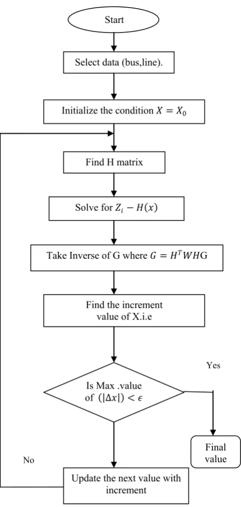
Absence of state estimation solution causes the occurrence of cascading failures or blackouts in local and/or regional areas for considerable time periods. The robustness and reliability of state estimation is a critical issue for power utilities. The Weighted Least Square (WLS) method is the commonly used state estimation approach which is used in power industries [17, 18]. In this paper weighted least square algorithm along with flow chart is presented and applied for IEEE 14-bus power system and for IEEE 30-bus power system.

(4)

Yes

No

Fig.1.Flow chart of WLS method.

III.PARTICLESWARMOPTIMIZATION

Particle swarm optimization (PSO) is a population-based optimization method first proposed by Kennedy and Eberhart in 1995, inspired by social behavior of bird flocking or fish schooling. The PSO as an optimization tool provides a population-based search procedure in which individuals called particles change their position (state) with time. In a PSO

system, particles fly around in a multidimensional search space.

During flight, each particle adjusts its position according to its own experience (This value is called pbest), and according to the experience of a neighboring particle (This value is called guest), made use of the best position encountered by itself and its neighbor (Fig. 2).

Fig .2. Concept of searching point by PSO

This modification can be represented by the concept of velocity. Velocity of each agent can be modified by the following equation:

𝑣𝑘+1= 𝑤. 𝑣𝑘+ 𝑐1𝑟𝑎𝑛𝑑 ∗ 𝑝𝑏𝑒𝑠𝑡 − 𝑥𝑘 + 𝑐2𝑟𝑎𝑛𝑑 ∗ 𝑔𝑏𝑒𝑠𝑡 − 𝑥𝑘

(21)

Using the above equation, a certain velocity, which gradually gets close to 𝑝𝑏𝑒𝑠𝑡 and 𝑔𝑏𝑒𝑠𝑡can be calculated.

The current position (searching point in the solution space) can be modified by the following equation:

𝑥𝑘+1_{= 𝑥}𝑘_{+ 𝑣}

𝑘+1,𝑘 = 1,2 … . 𝑛 (22)

Where

𝑥𝑘 _{is current searching point ,}_𝑥𝑘+1_{is modified searching}

point , 𝑣𝑘is current velocity , 𝑣𝑘+1 is modified velocity of

agent ,𝑉𝑝𝑏𝑒𝑠𝑡 is velocity based on 𝑝𝑏𝑒𝑠𝑡, 𝑉𝑔𝑏𝑒𝑠𝑡 is velocity based on 𝑔𝑏𝑒𝑠𝑡, 𝑛 is number of particles in a group, 𝑚 is number of members in a particle, 𝑝𝑏𝑒𝑠𝑡_𝑖 is 𝑝𝑏𝑒𝑠𝑡of agent 𝑘, 𝑔𝑏𝑒𝑠𝑡_𝑖 is 𝑔𝑏𝑒𝑠𝑡 of the group, w is weight function for velocity of agent 𝑘 , 𝑐𝑖 is weight coefficients for each term .

 c1 and c2 are two positive constants.

 r1 and r2 are two randomly generated numbers with a range of [0,1]

 𝑤 is the inertia weight and it is defined as a function of iteration index 𝑘as follows:

𝑤 𝑘 = 𝑤𝑚𝑎𝑥 − 𝑤𝑚𝑎𝑥_{𝑀𝑎𝑥 .𝐼𝑡𝑒𝑟}−𝑤𝑚𝑖𝑛 ∗ 𝑘 (23)

Where 𝑀𝑎𝑥. 𝐼𝑡𝑒𝑟, 𝑘 is maximum number of iterations and the current number of iterations, respectively. Start

Select data (bus,line).

Initialize the condition 𝑋 = 𝑋₀

Find H matrix

Solve for 𝑍_𝑖− 𝐻 𝑥

Take Inverse of G where 𝐺 = 𝐻𝑇_𝑊𝐻_G

∆𝑥 = 𝐺−1_𝐻𝑇_𝑊

Find the increment value of X.i.e

Is Max .value of ∆𝑥 < 𝜖

Update the next value with increment

Final value

Update velocities and position of each particle.

Evaluate the fitness value of each particle

(5)

To insure uniform velocity through all dimensions, the maximum velocity is as.

𝑣𝑚𝑎𝑥 ₌ 𝑥𝑚𝑎𝑥−𝑥𝑚𝑖𝑛

𝑁 (24)

Where N is a chosen number of iterations.

No

yes

No n

Yes

No

Yes

Fig 3.Flow chart of PSO

Step 1: The initial particles are generated randomly in the range of upper and lower limits of number of generators.

Step 2: The objective function and fitness value of each particle with its pbest is calculated. The best among the pbest is denoted as gbest.

Step 3: The velocity and position of each particle is updated according to equation (21) and (22) respectively.

Step 4: The objective function of each particle is compared with its pbest. If the current value is better than pbest then pbest value is set equal to the current value and pbest position is set equal to the current position.

Step 5: If the current fitness value is better than the gbest, then update gbest to current best position and fitness value

Step 6: Step 3 to 5 is repeated until the convergence criterion of maximum number of evaluations are met

Step 7: The individual that generates the latest gbest is the optimal generation power of each unit with the minimum total generation cost.

IV. DIFFERENTIAL EVOLUTION (DE)

Differential Evolution is an optimization algorithm that solves real-valued problems based on the principles of natural evolution [19]-[21]. DE uses a population P of size𝑁_𝑝, composed of floating point encoded individuals that evolve over G generations to reach an optimal solution. Each individual 𝑋𝑖 is a vector that contains as many parameters as

the problem decision variables D. The population size 𝑁_𝑝 is an algorithm control parameter selected by the user and it remains constant throughout the optimization process.

𝑃 𝐺 _{= 𝑋} 𝑖

𝐺 _{, … … , 𝑋} 𝑁𝑝

𝐺 ₍₂₅₎

𝑋_𝑖(𝐺)= 𝑋_1,𝑖 𝐺 , . . , 𝑋_𝐷,𝑖 𝐺 𝑇,𝑖 = 1, . . , 𝑁_𝑝 (26)

The optimization process in Differential Evolution is carried out with three basic operations: Mutation, Crossover and Selection. Differential Evolution starts by creating an initial population of 𝑁_𝑝 vectors, with random values assigned to each decision parameter in every vector as defined by (27).

𝑋_{𝑗 ,𝑖} 0 = 𝑋_𝑗𝑚𝑖𝑛 _{+ 𝜂}

𝑗 𝑋𝑗𝑚𝑎𝑥 − 𝑋𝑗𝑚𝑖𝑛 (27)

Where 𝑖 = 1, … , 𝑁𝑝 and 𝑗 = 1, … , 𝐷; 𝑋𝑗𝑚𝑖𝑛and 𝑋𝑗𝑚𝑎𝑥are the

lower and upper bounds of the 𝑗𝑡𝑕_{decision parameter and} 𝜂𝑗is a uniformly distributed random number within [0, 1]

generated a new for each value of j. 𝑋_{𝑗 ,1} 0 is the 𝑗𝑡𝑕_{parameter of}

the 𝑖𝑡𝑕_{individual of the initial population.}

Initialize the positions and velocities of each particle

Evaluate the fitness value of each particle

For each particle set local best fitness=current fitness and local best position=current position

Set global best fitness =min (local best fitness)

Set global best fitness=current fitness

Stopping criteria met?

Update velocities and position of each particle

Current fitness<local best fitness?

Set local best fitness=current fitness

Current fitness<global best fitness?

Set global best fitness=current fitness

Stop criteria met?

Stop Start

(6)

The mutation operator creates mutant vectors 𝑋𝑡′ by

perturbing a randomly selected vector 𝑋𝑎 with the

difference of two other randomly selected vectors 𝑋𝑏𝑎𝑛𝑑 𝑋𝑐 .

𝑋_𝑖′ 𝐺 = 𝑋_𝑎 𝐺 + 𝐹 𝑋_𝑏 𝐺 − 𝑋_𝑐 𝐺 , 𝑖 = 1, . . , 𝑁𝑝 (28)

Where 𝑋_𝑎, 𝑋_𝑏 𝑎𝑛𝑑 𝑋_𝑐 are randomly chosen vectors ∈ 1, . . 𝑁𝑝

and 𝑎 ≠ 𝑏 ≠ 𝑐 ≠ 𝑖. 𝑋_𝑎, 𝑋_𝑏 𝑎𝑛𝑑 𝑋_𝑐 are selected anew for each parent vector. The scaling constant (F) is an algorithm control parameter used to control the perturbation size in the mutation operator and improve algorithm convergence.

The crossover operation generates trial vectors 𝑋_𝑖" by mixing the parameters of the mutant vectors with the target vectors 𝑋𝑖 , according to a selected probability distribution.

𝑋_{𝑗 ,𝑖}" 𝐺 = 𝑋𝑗 ,𝑖 " 𝐺 _{, 𝑖𝑓 𝜂}

𝑗 ′ _{≤ 𝐶}

𝑅 𝑜𝑟 𝑗 = 𝑞

𝑋_{𝑗 ,𝑖} 𝐺 , 𝑜𝑡𝑕𝑒𝑟𝑤𝑖𝑠𝑒 (29)

Where 𝑖 = 1, … , 𝑁𝑝 and 𝑗 = 1, … , 𝐷;q is randomly chosen

index ∈ 1, . . 𝑁_𝑝 that guarantees that the trial vector gets at least one parameter from the mutant vector; 𝜂_𝑗′a uniformly distributed random number within [0, 1) generated anew for each value of j. Crossover constant 𝐶𝑅 is an algorithm control

parameter that controls the diversity of the population and aids the algorithm to escape from local optima. 𝑋_{𝑗 ,𝑖} 𝐺 , 𝑋_{𝑗 ,𝑖}′ 𝐺 𝑎𝑛𝑑 𝑋_{𝑗 ,𝑖}" 𝐺 are the 𝑗𝑡𝑕_{parameter of the}_𝑖𝑡𝑕_target

vector, mutant vector, and trial vector at generation G, respectively.

Finally, the selection operator forms the population by choosing between the trial vectors and their predecessors (target vectors) those individuals that present a better fitness or are more optimal according to (30).

𝑋_{𝑗 ,𝑖} 𝐺+1 = 𝑋𝑖

" 𝐺 _{, 𝑖𝑓 𝑓 𝑋} 𝑖

" 𝐺 _{≤ 𝑓 𝑋} 𝑖 𝐺

𝑋_{𝑗 ,𝑖} 𝐺 , 𝑜𝑡𝑕𝑒𝑟𝑤𝑖𝑠𝑒 , 𝑖 = 1, . . 𝑁𝑝

(30) This optimization process is repeated for several generations allowing individuals to improve their fitness as they explore the solution space in the search for optimal values.

DE has three essential control parameters: Scaling Factor 𝐹 , Crossover Constant 𝐶_𝑅 and Population Size 𝑁_𝑃. The scaling factor is a value in the range (0, 2] that controls the perturbation in the mutation process. The crossover constant is a value in the range [0, 1] that controls the diversity of the population. The population size determines the number of individuals in the population and provides the algorithm enough diversity to search the solution space.

A. Control Parameter Selection.

The most common method used to select control parameters is parameter tuning. Parameter tuning adjusts the control parameters through experimentation until the best settings are determined. Good initial value ranges for strategy DE/rand/1/bin are F= [0.5, 0.6],𝐶𝑅= 0.70.0.90 , 𝑁𝑝 = 3𝐷, 8𝐷 where D is the dimension or number of control variables of the problem being solved [22].

In general, to avoid premature convergence of the DE algorithm, it is crucial that F be of sufficient magnitude to counter act this selection pressure. On the other hand, the scaling factor F should not be chosen too large, since the number of function evaluations increases as F increases.

As mentioned previously, the crossover constant 𝐶𝑅

controls the diversity of the population. Relatively high values of 𝐶_𝑅 result in higher diversity and improved convergence speed. However, beyond a certain threshold value, the convergence rate may decrease or the population may converge prematurely. On the other hand, small values of 𝐶_𝑅 increase the possibility that the algorithm stagnates in local minima.

The population size plays an important role in the algorithm convergence rate. Small population may cause a poor searching performance and stagnations in local minima. Large populations increase the possibility for finding optimal solutions at the expense of a large number of function evaluations.

V. RESULTS.

Particle Swarm Optimization and Differential Evolution based Weighted Least Square State Estimation is tested on IEEE 14 bus system and IEEE 30 bus system. The true value of bus voltage for IEEE 14 bus system and estimated values of bus voltages with PSO and DE is tabulated in table.1. The true value of bus voltage for IEEE 30 bus system and estimated values of bus voltages with PSO and DE is tabulated in table2.

Table.1

Estimated states with PSO and DE for IEEE 14 Bus system.

Bus no. True

value V p.u

PSO estimated

Value V

p.u

DE estimated

value V

p.u 1.

2. 3. 4. 5. 6. 7. 8. 9.

1.0600 1.0450 1.0100 1.0000 1.0000 1.0700 1.0000 1.0900 1.0000

1.0600 1.0450 1.0100 0.9578 0.9614 1.0700 0.9919 1.0900 0.9763

(7)

Available online: https://edupediapublications.org/journals/index.php/IJR/ P a g e | 2810 10. 11. 12. 13. 14. 1.0000 1.0000 1.0000 1.0000 1.0000 0.9757 0.9931 1.0008 0.9939 0.9646 0.9758 0.9932 1.0009 0.9940 0.9647 Table.2

Estimated states with PSO and DE for IEEE 30 Bus system.

Bus No. True value V (p.u)

PSO estimated

value V

(p.u)

DE estimated

value V

(p.u) 1. 2. 3. 4. 5. 6. 7. 8. 9. 10. 11. 12. 13. 14. 15. 16. 17. 18. 19. 20. 21. 22. 23. 24. 25. 26. 27. 28. 29. 30. 1.0600 1.0430 1.0000 1.0600 1.0100 1.0000 1.0000 1.0100 1.0000 1.0000 1.0820 1.0000 1.0710 1.0000 1.0000 1.0000 1.0000 1.0000 1.0000 1.0000 1.0000 1.0000 1.0000 1.0000 1.0000 1.0000 1.0000 1.0000 1.0000 1.0000 1.0600 1.0430 0.9479 1.0600 1.0100 0.9400 0.9292 1.0100 0.9672 0.9476 1.0820 0.9750 1.0710 0.9564 0.9496 0.9560 0.9445 0.9356 0.9311 0.9344 0.9332 0.9376 0.9336 0.9236 0.9275 0.9075 0.9400 0.9403 0.9181 0.9056 0.9865 0.9700 0.9474 0.9384 0.9335 0.9395 0.9287 0.9449 0.9667 0.9472 1.0093 0.9746 0.9954 0.9559 0.9491 0.9555 0.9441 0.9352 0.9306 0.9339 0.9328 0.9372 0.9331 0.9231 0.9270 0.9070 0.9395 0.9398 0.9177 0.9051

Fig.4.comparision of Estimated values of bus voltages(V) with PSO and DE for IEEE 14 bus system

Fig.4.comparision of Estimated values of bus Voltages (V) with PSO and DE for IEEE 30 bus system.

VI.CONCLUSIONS.

The paper proposed the Particle Swarm Optimization and Differential Evolution for Power system State Estimation. Particle Swarm Optimization and Differential Evolution algorithm technique has been applied to Weighted Least Square State Estimation. Estimated Bus voltages values obtained for IEEE 14 bus system and 30 bus system through Particle Swarm Optimization are nearer to True Bus voltage value compared to Differential Evolution. The results of estimated Voltage values obtained through PSO and DE for IEEE 14 bus system and IEEE 30 bus system are tabulated in Table.1 and Table.2 and respected graphs are plotted as shown in Figure 3 and Figure 4 .

VII. REFERENCES.

[1] J. Grainger and W. D. Stevenson, Power System Analysis. New York: Mc-Graw-Hill, 1994.

[2] M. Crow, Computational Methods for Electric Power Systems, Boca Rat6n, Florida: CRC Press, 2002.

[3] Lars Holtcn, Andcrs Gjelsvik, SvcrreAam, Felix F. Wu and Wen-Hsiung E. Liu, ―Comparison of Different Methods for State Estimation‖, IEEE Transactions on Power Systems, Vol. 3, No. 4, pp. 1798-1806,November 1988.

[4] Kenneth I. Geisler and Anjan Bose, ―State Estimation Based External Network Solution for On-Line Security

0.8 0.9 1 1.1 1.2

1 3 5 7 9 11 13

V(p .u ) Bus No. PSO DE 0.8 0.9 1 1.1

1 4 7 10 13 16 19 22 25 28

(8)

Analysis‖, IEEE Transactions on Power Apparatus and Systems, Vol. PAS-102, No. 8, pp. 2447-2454,

August 1983.

[5] John J. Grainger and W.D. Stevenson JR, ―Power System Analysis‖,Tata McGraw Hill Edition, pp. 641-687, 2005. [6] M.A. Pai, ―Computer Technique in Power System Analysis‖, Second Edition, Tata McGraw-Hill Edition, pp. 39-53, 2006.

[7] Yun Yang, Wei Hu and Yong Min, ―Projected unscented Kalman filter for dynamic state estimation and bad data detection in power system‖,12th International Conference on Developments in Power System Protection (DPSP 2014), pp. 1-6, 31 Mar. - 3Apr.2014.

[8] Antonio de la Villa Jaeen and Antonio Goomez-Expoosito, ―Implicitly Constrained Substation Model for State Estimation‖, IEEE Transactions on Power Systems, Vol.17,No.3, pp. 850-856, Aug. 2002.

[9] Gabriele D. Antona, ―Uncertainty of Power System State Estimates due to Measurements and Network Parameter Uncertainty‖, IEEE International Workshop in Applied Measurements for Power Systems, pp. 37-40, 22-24 Sept. 2010.

[10] Allen J. Wood and Bruce F. Wollenberg, ―Power Generation, Operation, and Control‖, Second Edition, Wiley Student Edition, pp. 453- 508,2005.

[11] A. Monticelli and Felix F. Wu, ―A Method That Combines Internal State Estimation and External Network Modeling‖, IEEE Transaction on Power Apparatus and Systems, Vol. PAS-104, No. 1, pp. 91-103, Jan.1985.

[12] A. J. Wood and B. F. Wollenberg, Power Generation, Operation and Control, New York: Wiley, 1996.

[13] A. Monticelli, "Electric Power System State Estimation," Proceedings of the IEEE, vol. 88, no. 2, pp. 262-282,

February 2000.

[14] A. Abur and A. G6mez-Exp6sito, Power Systems State Estimation: Theory and Implementation, New York: Marcel Decker, Inc., 2004.

[15] A. Monticelli, State Estimation in Electric Power Systems: A Generalized Approach, Norwell, Massachusetts: Kluwer Academic Publishers, 1999.

[16] J.A. George and M.T. Heath, ―Solution of Sparse Linear Least Squares Problems using Givens Notations‖, Linear Algebra and Appl., Vol. 34, pp. 69-83, 1980.

[17] George N. Korres, ―A Robust Algorithm for Power System State Estimation with Equality Constraints‖, IEEE Transactions on Power Systems, Vol.25, no.3, pp. 1531-1541, Aug. 2010.

[18] Roberto Mínguez and Antonio J. Conejo, ―State Estimation Sensitivity Analysis‖, IEEE Transactions on Power Systems,Vol.22, no.3, pp. 1081-1091,Aug. 2007.

[19] K. Price, "Differential Evolution: A Fast and Simple Numerical Optimizer," Biennial Conference of the North American Fuzzy Information Processing Society. NAFIPS. 19-22 Jun 1996, pp. 524-527.

[20] R. Storm, "On the Usage of Differential Evolution for Function Optimization," Biennial Conference of the North

American Fuzzy Information Processing Society. NAFIPS. 19-22 Jun 1996, pp. 519-523.

[21] R. Storm, K. Price, "Differential Evolution - A simple and efficient adaptive scheme for global optimization over continuous spaces," [Online]. Journal of Global Optimization, vol. 11, Dordrecht, pp. 341-359, 1997.