Design of an Improved Star Configuration Based Statcom with H – Bridge Concept

(1)

Available online: https://edupediapublications.org/journals/index.php/IJR/ P a g e | 2182

Design of an Improved Star Configuration Based Statcom

with H – Bridge Concept

A. Suresh Kumar & P.Venkatesh

Department of Electrical and Electronics Engineering Samskruti College of Engineering &Technology Hyderabad, Telangana, INDIA.

[email protected] , [email protected]

Abstract: The main aim of this paper is to design a STATCOM which has the capability of compensating the fault and to overcome the conduction losses faced by the conventional STATCOM with traditional H-Bridge structure the future control procedures bestow themselves not only to the current loop control but also to the DC capacitor voltage control. With concerns to the current loop control, a nonlinear controller established on the passivity-based control (PBC) theory is used in this cascaded STATCOM. The capacitor voltage control, overall voltage control will control by embracing a proportional resonant controller. Clustered balancing mechanism will achieve by shifting the modulation wave vertically which can be easily executable in a field-programmable gate array. An artificial fault will be injected for a limited time period duration. Real and reactive power will be maintained for the compensated voltage and current. This work carried by using MATLAB /SIMULINK simulation tool.

1 INTRODUCTION

Now-a-days use of Flexible ac transmission systems (FACTS) devices have been increasing rapidly in power systems due to their power quality control, power transfer capacity of AC system interconnections. Shunt FACTS devices are utilized at point of common connection (PCC) to absorb or inject the reactive power into the power system. Due to this the voltage quality of PCC is improved. Out of all shunt devices static synchronous

compensator is preferred most due to its robust construction, wide range of voltage control, dynamic reactive current compensation and less response time. In recent years, many topologies have been applied to the STATCOM. Among these different types of topologies, H–Bridge Cascaded STATCOM is widely accepted for high power applications due to the following advantages:

 Quick response speed

 Small volume

 High efficiency

 Minimal interaction with the supply grid

 Individual phase control ability

2 CONFIGURATION OF STATCOM SYSTEM

The adjacent figure Fig. 4.1 shows the circuit of the star-configured STATCOM cascading 12 H-bridge pulse width modulation (PWM) converters in each phase and it can be expanded easily by adding more number of bridges or by removing the bridges according to the requirement. By controlling the current of STATCOM directly, it can absorb or provide the required reactive current to achieve the

purpose of dynamic reactive current

(2)

(a)

Fig. 1 Actual 10 KV 2 MVA H-bridge cascaded STATCOM. (a) Configuration of the system.

The power switching devices working in ideal condition is assumed. usa, usb and usc are

the three-phase voltage of grid. ua, ub, and uc are

the three-phase voltage of STATCOM. isa, isb,

and isc are the three-phase current of grid. ia, ib

and ic are the three-phase current of STATCOM.

ila, ilb and ilc are the three-phase current of load.

udc is the reference voltage of dc capacitor. C is

the dc capacitor. L is the inductor. Rs is the

starting resistor.

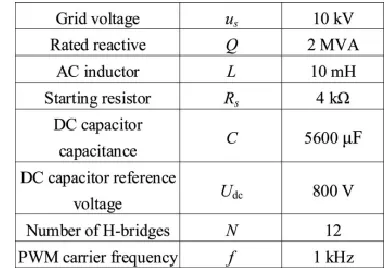
Table 4.1 summarizes the circuit parameters. The cascade number of N = 12 is assigned to H-bridge cascaded STATCOM, resulting in 36 H-bridge cells in total. Every cell is equipped with nine isolated electrolytic capacitors which the capacitance is 5600 μF. The dc side has no external circuit and no power source except for the dc capacitor and the voltage sensor. In each cluster, an ac inductor supports the difference between the sinusoidal voltage of the grid and the ac PWM voltage of STATCOM. The ac inductor also plays an important role in filtering out switch ripples caused by PWM. For selecting insulated-gate bipolar transistor (IGBT), considering the complexities of practical industrial fields, there might be the problems of the spike current and over load. Consequently, in order to ensure the stability and reliability of H-bridge cascaded

STATCOM, and also improve the over load capability, the current rating of the selected IGBT should be reserved enough safety margin. In the proposed system, 1.4 times rated current operation is guaranteed, the peak current under the 1.4 times over load condition is 224 A, the additional 76 A (30− 224 A = 76 A) is the safety margin of IGBT modules. Due to the previous considerations, the voltage and current ratings of IGBT which is selected as the switching element in main circuit are 1.7 kV and 300 A.

Table 1 Circuit Parameters of the simulation System

The modulation technology adopts the

carrier phase-shifted sinusoidal PWM

(abbreviated as CPS-SPWM) with the carrier frequency of 1 kHz. Then, with a cascade number of N = 12, the ac voltage cascaded results in a 25-level waveform in line to neutral and a 49-level waveform in line to line. In each cluster, 12 carrier signals with the same frequency as 1 kHz are phase shifted by 2π/12 from each other. When a carrier frequency is as low as 1 kHz, using the method of phase-shifted unipolar sinusoidal PWM, it can make an equivalent carrier frequency as high as 24 kHz. The lower carrier frequency can also reduce the switching losses to each cell.

3.CONTROL SYSTEM for H-BRIDGE CASCADED STATCOM

A system is a group of elements or

(3)

A control system is a system whose

response can be controlled by varying the input to the system. The output quantity is called controlled variable or response and the input quantity is called command signal or excitation.

There are two types of control systems. They are Open loop control and Closed loop control systems. The open loop control system has no feedback and it completely depends upon the input signal which we provide for the system to operate. It has robust construction, easy to operate, easy to design and highly economical. But the only defect is that it cannot vary the input signal according to the external disturbances caused during the system operation. Because of this the desired response is deteriorated when there are external disturbances.

Whereas in closed loop control system a feedback is provided to the input and an error signal is generated. This error signal changes the input according to the disturbances that are caused during the system operation. The external disturbances are also taken into account and the output is varied. Due to this the system becomes complicated and also loses its robust nature. It is also more costly than the open loop system.

Fig. 3 A Closed Loop Control System 4 NON – LINEAR CONTROL SYSTEM

Nonlinear control theory is the area of control theory which deals with systems that are nonlinear, time-variant, or both. Control theory is a branch of engineering that is concerned with inputs, and how to modify the output by changing the input using feedback. The system to be controlled is called the "plant". In order to make the output of a system follow a desired reference signal, a controller is designed which

compares the output of the plant to the desired output and provides feedback to the plant to modify the output and bring it closer to the desired output.

Linear control theory applies to systems made of linear devices; which means they obey the superposition principle; the output of the device is proportional to its input. Systems with this property are governed by linear differential equations. Nonlinear control theory covers a wider class of systems that do not obey the superposition principle. It applies to more real-world systems, because all real control systems are nonlinear. These systems are often governed by nonlinear differential equations.

An example of a nonlinear control system is a thermostat-controlled heating system. A building heating system such as a furnace has a nonlinear response to changes in temperature; it is either "on" or "off", it does not have the fine control in response to temperature differences that a proportional (linear) device would have. Therefore the furnace is off until the temperature falls below the "turn on" set point of the thermostat, when it turns on. Due to the heat added by the furnace, the temperature increases until it reaches the "turn off" set point of the thermostat, which turns the furnace off, and the cycle repeats. This cycling of the temperature about the desired temperature is called a limit cycle, and is characteristic of nonlinear control systems. There are specific properties of a Non – Linear Control System. They are:

 They do not obey the Superposition Principle.

 They do not exhibit linearity and homogeneity principles.

 They have multiple equilibrium points.  Solution to Non – Linear systems may

not exist for all times.

(4)

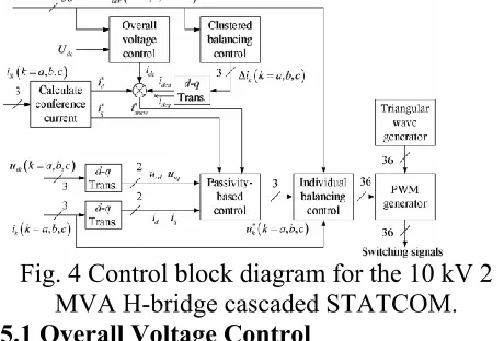
Fig. 4.4 shows a block diagram of the control algorithm for H-bridge cascaded STATCOM. The whole control algorithm mainly consists of four parts, namely, PBC, overall voltage control, clustered balancing control, and individual balancing control. The first three parts are achieved in DSP, while the last part is achieved in the FPGA.

Fig. 4 Control block diagram for the 10 kV 2 MVA H-bridge cascaded STATCOM. 5.1 Overall Voltage Control

As the first-level control of the dc capacitor voltage balancing, the aim of the overall voltage control is to keep the dc mean voltage of all converter cells equaling to the dc capacitor reference voltage. The common approach is to adopt the conventional PI controller which is simple to implement. However, the output voltage and current of H-bridge cascaded STATCOM are the power frequency sinusoidal variables and the output power is the double power frequency sinusoidal variable, it will make the dc capacitor also has the double power frequency ripple voltage. So, the reference current which is obtained in the process of the overall voltage control is not a standard dc variable and it also has the double power frequency alternating component and it will reduce the quality of STATCOM output current.

In general, when using Proportional Integral (PI) controller, in order to ensure the stability and the dynamic performance of system, the bandwidth of voltage loop control is set to be 200–500 Hz and it is difficult to

restrain the negative effect on the quality of STATCOM output current which is caused by the 100 Hz ripple voltage. Moreover, because of static error of PI controller, it will affect not only the first level control but also the second and the third one. Especially, during the startup process of STATCOM, it will make the voltage reach the target value with a much larger overshoot.

To resolve the problem, Proportional Resonant (PR) controller is adopted for the overall voltage control. The gain of the PR controller is infinite at the fundamental frequency and very small at the other frequency. Consequently, the system can achieve the zero steady-state error at the fundamental frequency. By setting the cutoff frequency and the resonant frequency of the PR controller appropriately, it can reduce the part of ripple voltage in total error, decrease the reference current distortion which is caused by ripple voltage, and improve the quality of STATCOM output current. Moreover, the dynamic performance and the dynamic response speed of the system also can be improved. In particular, during the startup process of STATCOM, the much larger dc voltage overshoot can be restrained effectively.

The PR controller is composed of a proportional regulator and a resonant regulator. Its transfer function or gain can be expressed as

(5)

increasing, the gain and the bandwidth of the controller are both increased.

We select the values kp = 0.05, kr = 10, ωc = 3.14 rad/s, and ω0 = 100π as the controller parameters. Fig. 4.5 shows the bode plots of the PR controller with the previous parameters and Fig. 4.6 shows the block diagram of overall voltage control. The signal of voltage error is obtained by comparing the dc mean voltage of all converter cells with the dc capacitor reference voltage. Then, the signal of voltage error is regulated by the PR controller and delivered to the current loop as a part of the reference current. Udc is the dc capacitor reference voltage. U*dc is the mean value of overall voltage. idc is the active control current for overall voltage control.

Fig. 5 Bode plots of the PR controller.

Fig. 6 Block diagram of overall voltage control. 5.2Clustered Balancing Control

Taking the clustered balancing control as the second level control of the dc capacitor voltage balancing, the purpose is to keep the dc mean voltage of 12 cascaded converter cells in eachcluster equaling the dc mean voltage of the three clusters. ADRC is adopted to achieve it. Then, it requires several steps to complete the design of ADRC for H-bridge cascaded STATCOM,which are as follows.

H-bridge cascaded STATCOM is a first order system; thus, the first-order ADRC is designed. Taking the dc capacitor voltage of each cluster as the controlled object for analysis, the

clustered balancing control model is built and the input and output variables and the controlled variable of the controlled object are determined. By using the nonlinear tracking differentiator (TD) which is a component of ADRC, the transient process for the reference input of the controlled object is arranged and its differential signal is extracted. Selecting the mean value of overall voltage U*dc as the reference voltage, TD is obtained via linear differential element and it can be expressed as

Where v1 is the tracking signal of reference voltage U*dc and v˙1 is the differential signal of the reference voltage U*dc. r1 is the speed tracking factor which reflects the changing rule of TD. The larger the r1, the faster the tracking speed and the larger the overshoot. Thus, it needs to select r1 properly according to the requirement of the actual system. α1 and δ1 are the adjustable control parameters. α1 determines the nonlinear form. The control effect will be changed greatly with the appropriate α1 . δ1 determines the size of the fal function linear range.

With the extended state observer (ESO) in ADRC, the uncertainties and the disturbances which lead to the unbalancing of the clustered dc capacitor voltages are observed and estimated dynamically.

The second-order ESO designed for the dc capacitor voltage of STATCOM could be written as

(6)

Ukdc (k = a, b, c) is the real-time detected value of the dc mean voltage of 12 cascaded converter cells in each cluster in current cyclical and it is used as known parameter. z1 is the state estimation signal of the dc capacitor voltage. ξ is the control deviation of the system. z2 is the internal and the external disturbance estimate signals of the controlled object. Δik is the control variable. b is the feedback coefficient of Δik (k = a, b, c). r21, r22, α2 , and δ2 are the adjustable control parameters. r22 has an effect on the delay of z2. The larger the r22, the smaller the delay. But, the larger r22 will lead to system oscillation. With r21 increasing slightly, the system oscillation could be damped. However, it will result in system divergence. Consequently, the adjustment of r21 and r22 requires mutual coordination. It can set r22 beforehand and then improve the control effect with increasing r21 gradually.

Actually, there are errors in the detection unit of the dc capacitor voltage of STATCOM. Thus, control precision of the dc capacitor voltage can be improved considerably by using z1 to estimate the state of the actual dc capacitor voltage precisely. For the changing of the system operation parameters in different applied environments, z2 can estimate the unknown disturbances accurately and optimize the dynamic response speed of the clustered balancing control. Whether the unknown disturbances can be estimated accurately with

ESO directly influences the control effect of ADRC. Therefore, the tuning of ESO parameters is very critical.

Nonlinear state error feedback (NLSEF) unit, a very important part of ADRC, is used to calculate the control variable of the active power adjustment for the clustered balancing control. However, in the practical application, the selection of NLSEF unit parameters in common ADRC is very difficult. Therefore, it is simplified with the linear optimization method in this paper and the newly obtained NLSEF unit can be expressed as

where fal function is defined above. ξ1 is the error value between the tracking signal v1 and the state estimation signal z1 . i0 is the control variable without the disturbance feedback compensation. b is the feedback coefficient which has relations with the control variable Δik and the state variable of the ESO. If the controlled object existed delay, with a larger b, it would generate a large error control signal making the response speed of the output faster and compensation of the internal and the external disturbances more effective. r3, α3, and δ3 are the adjustable control parameters. The regulating speed can be controlled by appropriately adjusting r3. However, the faster regulating speed might cause increased overshoot and system oscillation.

Finally, by combining NLSEF unit with the observed disturbances from ESO, the simplified ADRC can be achieved and then the clustered balancing control of H-bridge cascaded STATCOM can be realized. Fig. 4.7 shows a block diagram of the clustered balancing control with the simplified ADRC. When ADRC receives the reference voltage U*

(7)

real-Available online: https://edupediapublications.org/journals/index.php/IJR/ P a g e | 2188

time detected value of the dc mean voltage Ukdc (k = a, b, c) of 12 cascaded converter cells in each cluster, it will trace the reference voltage rapidly with TD and obtain the tracking signal v1 by filtering. Then, by subtracting the tracking signal v1 from the state estimation signal of the dc capacitor voltage z1, the control deviation command ξ1 of the system voltage is calculated. ξ1 is used as the input signal of NLSEF. Finally, the active adjustment control current Δik (k = a, b, c) of the clustered balancing control is achieved by subtracting the disturbance estimate signals which obtained in ESO from the output result i0 of NLSEF.

Fig. 7 Block diagram of clustered balancing control.

5.3 Individual Balancing Control

As the overall dc voltage and the clustered dc voltage are controlled and maintained, the individual control becomes necessary because of the different cells have different losses. The aim of the individual balancing control as the third level control is to keep each of 12 dc voltages in the same cluster equaling to the dc mean voltage of the corresponding cluster. It plays an important role in balancing 12 dc mean capacitor voltages in each cluster. Due to the symmetry of structure and parameters among the three phases, a-phase cluster is taken as an example for the individual balancing control analysis.

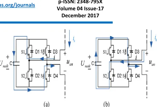
Fig. 4.8 shows the charging and discharging states of one cell. According to the polarity of output voltage and current of the cell, the state of the dc capacitor can be judged. Then, the dc capacitor voltage will be adjusted based on the actual voltage value.

Fig. 8 Charging and discharging states of one cell. (a) Charging state. (b) Discharging state.

As shown in Fig. 4.8, at some point, the direction of the current is from the grid to STATCOM. If S1 and S4 are open, the output voltage of the nth cell is positive. The current flows into the dc capacitor along the direction which is shown in Fig. 4.8(a) and charges the capacitor. Likewise, if S2 and S3 are open, the output voltage of the nth cell is negative. The current flows into the dc capacitor along the direction which is shown in Fig. 4.8(b) and discharges the capacitor. Obviously, to make the capacitor voltage of each cell tend to be consistent, the turn on time of the cell with the lower voltage should be extended and the turn-on time of the cell with the higher voltage should be shortened in charging state. Then, in discharging state, the process is contrary. The adjustment principle of the dc capacitor voltage can be summarized as follows.

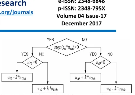
1. When (ia × uan ) > 0, if Unadc < Uadc, it needs to increase the duty cycle. If Unadc > Uadc, it needs to reduce the duty cycle. 2. When (ia × uan ) < 0, if Unadc > Uadc, it

(8)

According to the previous method, the direction and the magnitude of adjustment of the duty cycle for one cell can be achieved easily at some point.

Fig. 4.9 shows the adjustment method of the duty cycle by shifting the modulation wave vertically. Taking the first half period of the modulation wave as an example, the value of the modulation wave is greater than zero and the cell outputs zero level and 1 level. When the level is zero, the capacitor is not connected to the main circuit and it is not in the state of the charging and discharging. To reduce the charging time for one capacitor, it needs to reduce the action time of 1 level. And it can be realized by reducing the turn-on time of S1and S4 (as shown in Fig. 4.8). The state of the left bridge arm is decided by comparing the normal modulation wave with the triangular carrier. The state of the right bridge arm is decided by comparing the opposite modulation wave with the triangular carrier. Therefore, taking x-axis as the boundary, the duty cycle is reduced by shifting down the normal modulation wave and shifting up the opposite modulation wave according to

where eU dc = Unadc − Uadc. k is regulation coefficient. ui0 is the previous modulation wave. ui is the new modulation wave.

Fig. 9 Process of shifting modulation wave.

Fig. 10 Flowchart of shifting modulation wave. The previous principle is also suitable for reducing discharging time and prolonging the charging and discharging times of the cell. Summing up the previous analysis, the method can be illustrated as follows.

1.If the requirement is to reduce the duty cycle, it needs to shift down the normal modulation wave and shift up the opposite modulation wave.

2.If the requirement is to prolong the duty cycle, it needs to shift up the normal modulation wave and shift down the opposite modulation wave.

(9)

Fig. 11 Block diagram of individual balancing control.

5.4 Passivity Based Control

Passivity based control looks over clustered balancing control and overall voltage control. The output of clustered balancing control, ∆ik (k = a, b, c) is transformed to d-q form by d-q transformations. The direct current output i.e. idcd is considered and the quadrature current output idcq is earthed. Conference current is calculated from the load currents ilk(k = a, b, c) by d- q transformations and the direct current value i*d is considered. The output of overall voltage control idc is also considered. These three currents, idcd, i*d, idc are sent to the error detector and the error signal is sent to PBC as i*dnew.

The quadrature current value i*q of the conference current is also one of the inputs of PBC. The source voltages usk(k = a, b, c) are also transformed into d-q values and the outputs of these transformations usd and usq are fed to PBC. The line currents ik(k = a, b, c) are also transformed to id and iq values and are given as inputs to PBC.

Hence the six inputs of PBC block are i*dnew, id, i*q, iq, usd, ud out of which the latter two are voltage inputs where as the first four are current inputs. These current inputs are linked with the resistors and inductors and the output voltages are then compared to the voltage inputs. While linking with the inductors, differentiation of the current inputs is done. The reference voltages u*a, u*b, u*c are calculated by inverse d-q transformations of the calculated direct and quadrature voltages from these six inputs.

As shown in Fig. 4.12, the direct axis voltage ud is calculated by the summation of the following terms.

1. Direct axis source voltage usd

2. Negative product of inductor L and differentiated value of i*dnew, - L * (di*dnew/dt)

3. Negative product of resistor R and i*dnew, – R * i*dnew

4. Product of inductance ωL and i*q, ωL * i*q

5. Product of id and resistance Ra1, id * Ra1 ud = usd – L * (di*dnew/dt) – R * i*dnew + ωL * i*q + id * Ra1

As shown in Fig. 4.12, the quadrature axis voltage uq is calculated by the summation of the following terms.

1. Quadrature axis source voltage usq

2. Negative product of inductor L and differentiated value of i*q, - L * (di*q/dt) 3. Negative product of resistor R and i*q, -

R * i*q

4. Negative product of inductance ωL and current i*dnew, ωL * i*dnew

5. Product of resistor Ra2 and current iq, Ra2 * iq

uq = usq - L * (di*q/dt) - R * i*q + ωL * i*dnew + Ra2 * iq

Fig. 12 Block diagram of PBC.

Thus these two voltages ud and uq which are calculated as shown above are transformed to three phase voltages by inverse d-q transformations and then those transformed voltages are sent to the individual balancing control as shown in Fig. 4.4.

6. SIMULATION RESULTS

(10)

to the introduction of closed loop control system containing different control blocks for different modes of control. Although the injection of harmonics occurs due to the introduction of power electronic equipment, it is also compensated by active disturbances rejection controller (ADRC), thanks to the extended state observer (ESO) in the ADRC system.

The complete system is developed in MATLAB and simulated for the output results. The outputs of the MATLAB circuit are as expected and quite satisfactory. At first let us see the circuit developed in MATLAB. Fig. 5.1 is the MATLAB circuit for H-Bridge Cascaded STATCOM. Fig. 5.2 is the complete control block of H-Bridge Cascaded STATCOM.

Fig. 13 H-Bridge Cascaded STATCOM with 12 Bridges per phase.

Fig. 14 H-Bridge Cascaded STATCOM with Control Block.

Fig. 15 Three phase STATCOM current output.

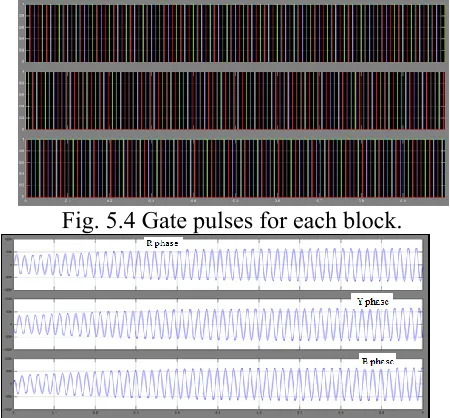
Fig. 5.4 Gate pulses for each block.

Fig. 16 Load current Pulses after STATCOM.

Fig 17. Source voltage and STATCOM Voltage Pulses.

Fig. 18 Individual Capsule of H-Bridge

Section IV: CONCLUSION

(11)

control methods are also proposed in detail. The proposed methods have the following characteristics.

A PBC theory-based nonlinear controller is first used in STATCOM with this cascaded structure for the current loop control, and the viability is verified by the simulation results.

The PR controller is designed for overall voltage control and the simulation result proves that it has better performance in terms of response time and damping profile compared with the PI controller.

The ADRC is first used in H-bridge cascaded STATCOM for clustered balancing control and the simulation results verify that it can realize excellent dynamic compensation for the outside disturbance.

The individual balancing control method which is realized by shifting the modulation wave vertically can be easily implemented in the FPGA.

The simulation results have confirmed that the proposed methods are feasible and effective. In addition, the findings of this study can be extended to the control of any multilevel voltage source converter, especially those with H-bridge cascaded structure.

REFERENCES

[1] B. Gultekin and M. Ermis, ―Cascaded multilevel converter-based transmission STATCOM: System design methodology and development of a 12 kV±12 MVAr power stage,‖IEEE Trans. Power Electron., vol. 28, no. 11, pp. 4930–4950, Nov. 2013.

[2] B. Gultekin, C. O. Gerc ¸ek, T. Atalik, M. Deniz, N. Bic¸er, M. Ermis, K. Kose, C. Ermis, E. Koc¸, I. C ¸ adirci, A. Ac ¸ik, Y. Akkaya, H. Toygar, and S. Bideci, ―Design and implementation of a 154-kV±50- Mvar transmission STATCOM based on 21-level cascaded multilevel converter,‖IEEE Trans. Ind.

Appl., vol. 48, no. 3, pp. 1030–1045, May/Jun. 2012. [3] S. Kouro, M. Malinowski, K. Gopakumar, L. G. Franquelo, J. Pou, J. Rodriguez, B. Wu, M. A. Perez, and J. I. Leon, ―Recent advances and industrial applications of multilevel converters,‖IEEE Trans. Ind. Electron., vol. 57, no. 8, pp. 2553–2580, Aug. 2010.

[4] F. Z. Peng, J.-S. Lai, J. W. McKeever, and J.

VanCoevering, ―A multilevel voltage-source inverter with separate DC sources for static var generation,‖ IEEE

Trans. Ind. Appl., vol. 32, no. 5, pp. 1130– 1138, Sep./Oct. 1996.

[5] Y. S. Lai and F. S. Shyu, ―Topology for hybrid multilevel inverter,‖Proc. Inst. Elect. Eng.—Elect. Power Appl., vol. 149, no. 6, pp. 449–458, Nov. 2002.

[6] D. Soto and T. C. Green, ―A comparison of highpower converter topologies for the implementation of FACTS controllers,‖IEEE Trans. Ind. Electron., vol. 49, no. 5, pp. 1072–1080, Oct. 2002.

[7] C. K. Lee, J. S. K. Leung, S. Y. R. Hui, and H. S.-H. Chung, ―Circuit-level comparison of STATCOM technologies,‖IEEE Trans. Power Electron., vol. 18, no. 4, pp. 1084–1092, Jul. 2003.

[8] H. Akagi, S. Inoue, and T. Yoshii, ―Control and performance of a transformerless cascade PWM STATCOM with star configuration,‖ IEEE Trans. Ind. Appl., vol. 43, no. 4, pp. 1041–1049, Jul./Aug. 2007. [9] A. H. Norouzi and A. M. Sharaf, ―Two control scheme to enhance the dynamic performance of the STATCOM and SSSC,‖IEEE Trans. Power Del., vol. 20, no. 1, pp. 435–442, Jan. 2005.

[10] C. Schauder, M. Gernhardt, E. Stacey, T. Lemak, L. Gyugyi, T. W. Cease, and A. Edris, ―Operation of±100 MVAr TVA STATCOM,‖IEEE Trans. Power Del., vol. 12, no. 4, pp. 1805–1822, Oct. 1997.

[11] C. H. Liu and Y. Y. Hsu, ―Design of a selftuning PI controller for a STATCOM using particle swarm optimization,‖IEEE Trans. Ind. Electron., vol. 57, no. 2, pp. 702–715, Feb. 2010.

[12] S. Mohagheghi, Y. Del Valle, G. K. Venayagamoorthy, and R. G. Harley, ―A proportional-integrator type adaptive critic designbased neurocontroller for a static compensator in a multimachine power system,‖ IEEE Trans. Ind. Electron., vol. 54, no. 1, pp. 86–96, Feb. 2007.