A Novel Nested Array Design for Direction of Arrival Estimation
of Noncircular Signals
Weijian Si, Zhanli Peng, Changbo Hou*, and Fuhong Zeng
Abstract—In this paper, a novel nested array is proposed for direction of arrival (DOA) estimation of noncircular signals. By using the noncircular property, we can get a virtual array composed of difference coarray (DCA) and sum coarray (SCA). Specifically, we give the properties of DCA and SCA for the generalized translational nested array first. Then, based on the relationship between DCA and SCA, an optimal translational nested array with increased degrees of freedom (DOFs) is constructed. To extend the physical array aperture, we move part of sensors in the translational nested array to the mirrored locations. Accordingly, the novel nested array with increased DOFs and physical array aperture is obtained. Finally, superiority of the proposed array is demonstrated by simulation experiments.
1. INTRODUCTION
Sparse arrays have attracted considerable attention from researchers in recent years due to their large inter-element spacing and underdetermined direction of arrival (DOA) estimation ability [1–5]. Typical sparse arrays, such as minimum redundancy arrays (MRAs) [6], nested arrays (NAs) [1], and coprime arrays (CPAs) [7], can resolve O(N2) sources with O(N) physical sensors. Accordingly, many modified versions [8–10] of the above sparse arrays have been presented, where their virtual arrays consist only of difference coarray (DCA), i.e., only the property of circular signals is considered.
However, in practical applications, lots of noncircular signals also exist, e.g., binary phase shift keying (BPSK), pulse amplitude modulation (PAM), and minimum shift keying (MSK), etc.. Research results in [11] indicate that the ellipse covariance matrix of noncircular signals is not equal to zero, which means that they can be exploited for DOA estimation combined with the covariance matrix. Thus, based on this property, many DOA estimation methods for noncircular signals were proposed, such as noncircular Root-MUSIC [11], noncircular ESPRIT [12], and MUSIC-Like method [13], etc. However, the above methods can only be used in uniform linear arrays (ULAs) for DOA estimation, which indicates that only 2(N −1) noncircular signals can be detected withN physical sensors.
Recently, some DOA estimation methods about noncircular signals based on sparse arrays have been proposed to improve the DOA estimation performance. In [14], the researchers presented an ambiguity-free DOA estimation method for unfold CPA. By using the coprime property of unfold CPA, the ambiguity problem is suppressed effectively. Nevertheless, only at most 2(M+N −1) noncircular signals can be detected when a unfold CPA with M +N −1 physical sensors is used. Since the noncircular signals possess non-zero ellipse covariance matrix, it can be vectorized to generate the sum coarray (SCA) [15–17]. Therefore, based on this, some subspace-based [15, 17] and compressive sensing-based [16, 18] underdetermined DOA estimation methods for noncircular signals have also been proposed. Through the joint use of DCA and SCA, the number of continuous virtual sensors extended by these sparse arrays can be increased dramatically, which can further contribute to the improvement of DOA estimation performance. For convenience, we name the number of continuous virtual sensors as
Received 4 October 2019, Accepted 23 November 2019, Scheduled 9 December 2019
* Corresponding author: Changbo Hou ([email protected]).
continuous degrees of freedom (cDOFs). Note that, the above DOA estimation methods are proposed based on the prototype NA and CPA, whose physical structures are not optimal for the DOA estimation of noncircular signals.
To achieve the underdetermined DOA estimation of noncircular signals with increased cDOFs, diff-sum coprime array with multiperiod subarrays (DsCAMpS) is proposed in [17]. By complementing DCA with SCA, the cDOFs of DsCAMpS is increased compared to that of traditional CPA. However, high redundancy between DCA and SCA indicates that DsCAMpS is not optimal. Thus, some new sparse array design strategies inspired by nested concept have been presented. In [15], a new nested array (NNA) with sum and difference composite coarray (SDCA) is introduced, which owns larger cDOFs than prototype NA. Unfortunately, we cannot get such NNA when the total sensor number is odd. To overcome this drawback, a nested array with displaced subarray (NADiS) is designed in [19]. By redefining the distance between dense subarray and sparse one, and expanding the inter-element spacing of sparse subarray in the protype NA, NADiS owns significantly increased cDOFs and physical array aperture. In [20], exhaustion method is utilized to determine the optimal sparse array configuration for noncircular signals (SANC). Although SANC has achieved the maximum cDOFs, it does not possess explicit closed-form expression. What is more, some holes exist in the SDCAs of the above sparse arrays, which will restrict the DOA estimation performance for noncircular signals.
In this paper, we propose a novel nested array for DOA estimation of noncircular signals. This novel configuration not only possesses the same advantage as prototype NA, i.e., continuous virtual array, but also owns almost twice more cDOFs than the latter [1]. In addition, the physical aperture of the proposed array is also increased, which can improve the DOA estimation performance further. To obtain this novel nested array, we first give the generalized definition of translation nested array (TNA) [21]. Its corresponding properties of DCA and SCA are also introduced. Then, based on the relationship between DCA and SCA, we can determine the optimal translation distances for TNA to maximize the obtaining cDOFs. By flipping part of sensors in the optimal TNA to the negative axis, we can get the proposed array, which owns a much larger physical aperture than the optimal TNA. In the end, the DOA estimation performance of the proposed array is evaluated through simulation experiments.
The remainder of this paper is organized as follows. Section 2 reviews the system model for DOA estimation of noncircular signals. Section 3 introduces the proposed novel nested array. Simulation experiments are provided in Section 4. Section 5 concludes this paper.
2. SYSTEM MODEL
For an N-sensor TNA, the sensor position sets of its subarray 1 and subarray 2 can be respectively
denoted as
P1={(p1+a1)d|a1 ∈Z, p1 = 1, . . . , N1}
P2={(p2(N1+ 1) +a2)d|a2 ∈Z, p2 = 1, . . . , N2}
(1)
whereZis the integer set. a1dand a2drepresent the translation distances for subarray 1 and subarray
2, respectively. N1 andN2 are the corresponding sensor numbers, whereN1+N2=N. Without loss of
generality, the unit inter-element spacingdis fixed as half a wavelength. Obviously, the prototype NA is a special case of TNA with a1 =a2 = 0.
Assume K uncorrelated far-field narrowband noncircular signals impinge on the N-sensor TNA, where the DOA of the kth signal is θk∈[−π/2, π/2). Then, the array output at thetth snapshot can
be expressed as
x(t) =
K
k=1
a(θk)sk(t) +n(t) (2)
where a(θk) = [ej2πl1sinθk/λ, . . . , ej2πlNsinθk/λ]T denotes the steering vector of the kth signal, and
[]T represents the transpose operation. [l1, . . . , lN] is the sensor position set, which satisfies ln ∈
P1 ∪P2, n = 1, . . . , N. sk(t) represents the kth noncircular signal at the tth snapshot, and n(t)
is the additive Gaussian white noise vector. It is obvious from the noncircularity of sk(t) that
ρk ∈ (0,1] denotes the corresponding noncircular rate. E[sk(t)s∗k(t)] = σk2 is the kth signal power, and E[] is the expectation operation. Besides, the signal and noise are assumed to be statistically independent.
Then, the covariance matrix ofx(t) can be denoted as
Rx = Ex(t)xH(t)=ARsAH+σn2I (3)
where A = [a(θ1), . . . ,a(θK)] is the manifold matrix. Rs = diag[σ12, . . . , σK2 ] is the signal covariance
matrix. σn2I and I respectively denote the noise covariance matrix and the N-dimensional identity matrix. The symbol ()H denotes the conjugate transpose operation. For convenience of analysis, noncircular phases and rates for all signals are assumed to be zero and one, respectively. Under this condition, the ellipse covariance matrix of x(t) and its conjugate can be respectively given as
Γx = Ex(t)xT(t)=ARsAT (4)
Γ∗x = Ex∗(t)xH(t)=A∗RsAH (5)
In practice, Rx, Γx, and Γ∗x are estimated by the maximum likelihood method, where the array output data with T snapshots is used. Combining Eqs. (3), (4), and (5), we can get the following expression
R=
R
x Γx Γ∗x
=
⎡
⎣ ARsA
H
ARsAT A∗RsAH
⎤
⎦+
⎡
⎣ σ
2 nI 0 0
⎤
⎦ (6)
where0 denotes the N×N zero matrix. Vectorizing Eq. (6), we have
z= vec(R) =Bp+σ2n1 (7)
where B = [(A∗A)T,(AA)T,(A∗A∗)T]T and the symbol denotes the Khatri-Rao product.
p = [σ12, . . . , σ2K]T, and 1 = [¯IT,0¯T,0¯T]T. ¯I and ¯0 are the vectorization of I and 0, respectively. It is
clear that Eq. (7) can be regarded as a virtual array data model with only a single snapshot. Then, the corresponding virtual sensor positions can be expressed as
V=D∪S∪ −S (8)
where D = {li − lj|li, lj ∈ P1 ∪ P2} is the DCA. The union of S and −S is the SCA, where
S={li+lj|li, lj ∈P1∪P2}. Vdenotes the SDCA.
After removing the repeated elements inV, we can get the consecutive part U. Then, cDOFs of V is
cDOFs =|U| (9)
whereU⊆V, and the symbol ||refers to the cardinality of a set.
Then, the virtual array output corresponding toUcan be formulated as
z0 =B0p+σ2n10 (10)
Based on Eq. (10), spatial smoothing MUSIC (SS-MUSIC) [3] can be used to estimate the DOAs. Note that the above description is a special case for DOA estimation of noncircular signals. When the noncircular phases are not zero or the noncircular rates are less than one, the corresponding DOA estimation methods based on sparse arrays can be found in [16, 17].
3. PROPOSED NOVEL NESTED ARRAY FOR NONCIRCULAR SIGNALS
In this section, we first introduce the design strategy for the proposed novel nested array. Then, its properties about cDOFs and physical array aperture are analyzed. Note that, the parameterdis ignored in the remainder of this paper to simplify the analysis.
According to Eq. (1), we can give the definition of generalized TNA as follows.
Definition 1: Given the parameters N1 and N2, the generalized TNA is defined as
P
1 ={p1+a1|a1 ∈Q, p1 = 1, . . . , N1}
P2 ={p2(N1+ 1) +a2|a2∈Q, p2 = 1, . . . , N2}
whereQ is the rational number set.
From [21], we know that TNA has the potential to increase cDOFs when its sensors are laid out properly. In addition, it can be seen from [2] that the offset configuration of two-dimensional NA can generate more virtual sensors. Accordingly, we deduce that generalized TNA may have the similar property. According to [21], we obtain the following property of generalized TNA.
Property 1: For generalized TNA in Definition 1, its DCA has the same form as that of NA when
a1=a2 ∈Qor a1 =a2+ (N1+ 1)N2 ∈Q.
The proof can be found in Appendix A. Obviously, the DCAs of generalized TNA and traditional NA are identical as long asa1 anda2 have the relationship in Property 1. Under this case, the DCA of
generalized TNA can be expressed as
D={−(N1+ 1)N2+ 1, . . . ,(N1+ 1)N2−1} (12)
Besides, the continuous part of SCA for generalized TNA can be denoted as
U1
SCA=U1∪ −U1, if a1=a2 ∈Q
U2
SCA=U2∪ −U2, if a1=a2+ (N1+ 1)N2 ∈Q
(13)
whereU1={2 + 2a2, . . . , M+ 2a2},U2 ={M+ 2a2, . . . ,2M−2 + 2a2}, andM = (N1+ 1)(N2+ 1). It
is clear from Eq. (13) that the SCA can be utilized to improve the underdetermined DOA estimation performance of noncircular signals.
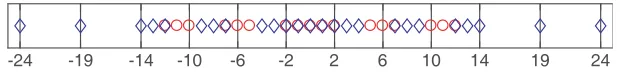
From Eq. (8), we know that SDCA is the union of DCA and SCA. Some repeated elements between DCA and SCA always exist for the presented sparse arrays [15, 17, 19, 20], which will decrease the available cDOFs. Fig. 1 provides an example of NADiS to illustrate this phenomenon, where the number of physical sensors is fixed to be 5. The physical sensor positions are specified as{0,1,2,7,12}. The DCA and SCA can be respectively denoted as D = {0,±1,±2,±5,±6,±7,±10,±11,±12} and
S={0,±1,±2±3,±4,±7,±8,±9,±12,±13,±14,±19,±24}. Obviously, we can find that the repeated elements betweenDand Sare{0,±1,±2,±7,±12}. In addition, it is obvious that the SDCA of NADiS is discontinuous. From the above analysis, we know that the cDOFs may increase significantly after the corresponding discontinuous parts of SDCA and the repeated elements between DCA and SCA are eliminated.
-24 -19 -14 -10 -6 -2 2 6 10 14 19 24
Figure 1. The DCA and SCA of NADiS with 5 physical sensors, where red circles and blue rhombuses denotes the elements in DCA and SCA, respectively.
Reviewing the offset configuration of two-dimensional NA [2], we can find that the cross-difference result between the dense subarray and sparse subarray is essentially the cross-sum. Obviously, its virtual array is the union of DCA and SCA in nature, i.e., SDCA. Compared with sensor configurations I and II in [2], the offset configuration can not only generate the continuous SDCA, but also can achieve the largest cDOFs. Inspired by this finding, we obtain the following property.
Property 2: When a1 = a2 = −(N1 + 1)(2N2 + 1)/2, or a1 = (N1 + 1)(2N2 − 1)/2 and
a2=−(N1+ 1)/2, the generalized TNA can generate the continuous SDCA with the maximum cDOFs,
i.e., cDOFs = 2(N1+ 1)(2N2+ 1)−3.
The proof of Property 2 is omitted here since it has a similar process to that described in Appendix B of [21]. From Property 2, we know that there are two different cases for a1 and a2 to achieve the
same and maximum cDOFs. That is to say, there are no repeated elements between DCA and SCA. For the first case, i.e., a1 = a2 = −(N1 + 1)(2N2+ 1)/2, the specific expressions of generalized TNA
can be denoted as
PS1,1={p1−(N1+ 1)(2N2+ 1)/2|p1 = 1, . . . , N1}
PS1,2={(p2−(2N2+ 1)/2)(N1+ 1)|p2= 1, . . . , N2} (14)
of generalized TNA can be modified as
PS2,1={p1−N1−1 + (N1+ 1)(2N2+ 1)/2|p1 = 1, . . . , N1}
PS2,2={(p2−N2−1 + (2N2+ 1)/2)(N1+ 1)|p2= 1, . . . , N2}
(15)
Observing Eqs. (14) and (15), we can find thatPS1,1 =−PS2,1 and PS1,2=−PS2,2. Then, it is easy
to know that the generalized TNAs under this two cases are mirror symmetric about zero point. Based on the above analysis, the proposed novel nested configuration can be defined as follows.
Definition 2: Given parameters N1 and N2, the proposed novel nested array can be defined as
P1=f{p1+ (N1+ 1)(2N2−1)/2|p1 = 1, . . . , N1}
P2=f{p2(N1+ 1)−(N1+ 1)/2|p2 = 1, . . . , N2}
(16)
where the operation f{} is defined as f{x1, x2, x3, x4, . . .}={x1,−x2, x3,−x4, . . .}.
From Definition 2, we can easily determine the physical array aperture as
LPA= (N1+ 1)(2N2+ 1)−3 (17)
To achieve the maximum cDOFs for the fixed physical sensor number, we need to solve the following optimization equation:
max
N1,N2∈Z+
2(N1+ 1)(2N2+ 1)−3
subject to: N1+N2 =N
(18)
It is easy from Eq. (18) to know that the optimal solutions are
N1 = (N −1)/2, N2 = (N+ 1)/2, N is odd
N1 =N2 =N/2, N is even
(19)
According to Eq. (19), we can obtain the corresponding expressions of cDOFs and physical array aperture as
cDOFs = N2+ 3N −1 (20)
LPA = (N2+ 3N −4)/2 (21)
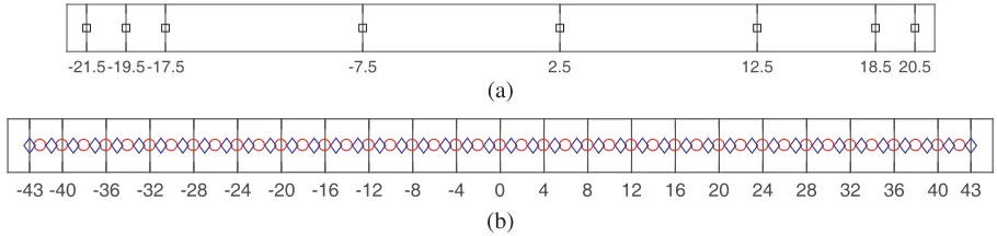
An example is shown in Fig. 2, whereN = 8. From Eq. (19), we can determine thatN1=N2= 4.
Then, the physical sensor position sets of the proposed array are P1 = {18.5,−19.5,20.5,−21.5},
and P2 = {2.5,−7.5,12.5,−17.5}. It can be seen from Fig. 2(a) that the physical array aperture of
proposed array is equal to 42. Fig. 2(b) gives the corresponding virtual array, which is continuous. More importantly, the union of DCA and SCA does not have repeated elements, which can help to increase the cDOFs. From Fig. 2(b), we know that the number of cDOFs is equal to 87. The above results is in accordance with Eqs. (16), (19)–(21).
-21.5 -19.5 -17.5 -7.5 2.5 12.5 18.5 20.5
(a)
-43 -40 -36 -32 -28 -24 -20 -16 -12 -8 -4 0 4 8 12 16 20 24 28 32 36 40 43
(b)
Figure 2. An example of the proposed novel nested array with 8 physical sensors. (a) Physical sensors distribution of the proposed array, whereP1={18.5,−19.5,20.5,−21.5}, P2 ={2.5,−7.5,12.5,−17.5}.
4. SIMULATION RESULTS
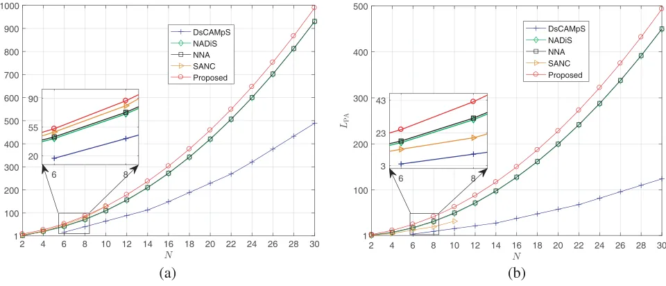
In this section, we select NNA [15], DsCAMpS [17], NADiS [19], and SANC [20] as the comparison arrays. To demonstrate the superiority of the proposed array, cDOFs and physical array aperture of the proposed array are first studied. Then, normalized spectrum of the proposed array is provided to verify the DOA estimation validity. In the end, we give the root-mean-squared error (RMSE) results to evaluate the DOA estimation performance of the proposed array for noncircular signals. It should be noted that the unit inter-element spacing is set as half a wavelength in the following experiments.
4.1. cDOFs and Physical Array Aperture
In the first experiment, we study the cDOFs and physical array aperture of the proposed array. Let the total physical sensor number N vary from 2 to 30. According to the definitions of NNA, DsCAMpS, NADiS, and the proposed array, we can determine their specific sensor position sets respectively. Note that SANC is obtained by exhaustion method. Hence, its configurations are provided under the condition of 2≤N ≤10.
Figure 3(a) shows the comparisons about cDOFs, while Fig. 3(b) depicts the curves about physical array aperture. It can be seen from Fig. 3 that the proposed array possesses larger cDOFs and physical array aperture than the other comparison arrays. Thus, the proposed array can identify more noncircular signals and owns better estimation performance in comparison with NNA, DsCAMpS, NADiS, and SANC.
2 4 6 8 10 12 14 16 18 20 22 24 26 28 30 1
100 200 300 400 500 600 700 800 900 1000
cDOFs
DsCAMpS NADiS NNA SANC Proposed
6 8
20 55 90
(a) (b)
2 4 6 8 10 12 14 16 18 20 22 24 26 28 30 1
100 200 300 400 500
DsCAMpS NADiS NNA SANC Proposed
6 8
3 23 43
Figure 3. Comparisions of (a) cDOFs, (b) physical array aperture.
4.2. Normalized Spectrum
In the second experiment,N is fixed to be 8 to show the DOA estimation effectiveness of the proposed array. According to Fig. 2(a), we know that the physical sensor positions of the proposed array are
{−21.5,−19.5,−17.5,−7.5,2.5,12.5,18.5,20.5}. Consider that K = 41 BPSK signals with uniform distribution between −60◦ and 60◦ impinge on this array. Both SNR and snapshots are considered ideal, i.e., the array output data is noiseless and possesses infinite number of snapshots. Then, SS-MUSIC with 0.01◦ search interval is used to estimate the DOAs.
-90 -60 -30 0 30 60 90
(degree)
0 0.2 0.4 0.6 0.8 1
Normalized Spectrum
Figure 4. Normalized spectrum of the proposed array, whereN = 8, andK = 41.
4.3. RMSE
To further evaluate the DOA estimation performance of the proposed array, RMSE experiments are conducted in this subsection. Similar to the previous subsection, N is set to 8. Then, the sensor positions of NNA, DsCAMpS, NADiS, and SANC can be respectively given as{0,1,2,3,11,18,25,32},
{0,2,3,4,6,8,9,10}, {0,1,2,3,4,13,22,31}, and{0,6,12,15,16,17,19,20}. The sensor positions of the proposed array are the same as that in the previous subsection. Thus, the cDOFs of the above five sparse arrays are 73, 41, 71, 81, and 87, respectively. In addition, the corresponding physical array apertures can be respectively given as 32, 10, 31, 20, and 42. Assume that there are K = 15 BPSK signals with uniform distribution between −60◦ and 60◦ impinging on the above arrays. The DOA estimation method and search interval keep unchanged compared with the previous experiment. Then, we can know that the number of identifiable noncircular signals for NNA, DsCAMpS, NADiS, SANC,
-10 -5 0 5 10 15 20
0.07 0.1 0.14 0.21 0.3 0.45 0.65
RMSE (degree)
DsCAMpS NADiS NNA SANC Proposed
100 200 300 400 500 600 700 800 900 1000 0.06
0.1 0.18 0.3 0.54 0.9 1.6
RMSE (degree)
DsCAMpS NADiS NNA SANC Proposed
(a) (b)
and the proposed array are 36, 20, 35, 40, and 43, respectively. The RMSE results are calculated according to the following expression:
RMSE =
1
IK
I
i=1 K
k=1
ˆ
θk(i)−θk
2
(22)
where I = 500 is the number of Monte Carlo trials, and ˆθk(i) is the estimated DOA of θk in the ith
trial.
Figure 5(a) shows the RMSE curves as a function of SNR, where the number of snapshots is fixed as 500. Fig. 5(b) is the RMSE results versus snapshots under the condition of SNR = 0 dB. It can be observed from Fig. 5 that the RMSE curves of all sparse arrays decrease as the increase of SNR and snapshots. Moreover, the proposed array always possesses less RMSE than the other four arrays, especially in the case of high SNR and snapshots. The reason is that the cDOFs and physical array aperture of the proposed array are larger than those of NNA, DsCAMpS, NADiS, and SANC. Thus, we can conclude that our proposed array possesses the best DOA estimation performance among all the five sparse arrays.
5. CONCLUSION
In this paper, we have proposed a novel nested array for DOA estimation of noncircular signals. Before giving this novel sparse array, we first introduce the generalized TNA concept. Then, the relationship between DCA and SCA is investigated. By using the properties of generalized TNA, we finally construct the proposed array configuration. In addition, the optimal selections of N1 and N2 are also provided
so as to achieve the maximum cDOFs and the largest physical aperture. Finally, simulation results demonstrate the superiority of the proposed array for the DOA estimation of noncircular signals.
APPENDIX A. PROOF OF PROPERTY 1
From [8, 21], we know that the DCA of a sparse array can be expressed as the union of its self-difference and cross-difference. Thus, the DCA of the generalized TNA can be expressed as
D= (P1−P1)∪(P2−P2)∪(P1−P2)∪(P2−P1) (A1)
whereP1 ={p1+a1|a1 ∈Q, p1 = 1, . . . , N1} andP2 ={p2(N1+ 1) +a2|a2 ∈Q, p2 = 1, . . . , N2}. Then,
we have
P1−P1 = {−N1+ 1,−N1+ 2, . . . , N1−2, N1−1} (A2)
P2−P2 = {−(N2−1)(N1+ 1),−(N2−2)(N1+ 1), . . . ,(N2−2)(N1+ 1),(N2−1)(N1+ 1)}(A3)
P2−P1 = {p2(N1+ 1)−p1+a2−a1|a1, a2 ∈Q, p1 = 1, . . . , N1, p2 = 1, . . . , N2} (A4)
In addition, it is obvious from Eq. (A1) thatP1−P2 and P2−P1 are mirror symmetric about zero
point. Observing Eq. (11), we can find that the generalized TNA will become the traditional NA when a1=a2 = 0. Accordingly, the DCA of NA can be expressed as
DNA= (P1−P1)∪(P2−P2)∪(P1,0−P2,0)∪(P2,0−P1,0) (A5)
whereP2,0−P1,0=−(P1,0−P2,0) ={p2(N1+ 1)−p1|p1 = 1, . . . , N1, p2 = 1, . . . , N2}. For convenience
of analysis, let Up2 ={p2(N1+ 1)−p1|p1= 1, . . . , N1}. It is apparent thatUp2 is fully continuous and
possessesN1 elements. Then, the cross-difference existing in Eq. (A5) can be denoted as
(P1,0−P2,0)∪(P2,0−P1,0) =−UN2∪ −UN2−1∪. . .∪UN2−1∪UN2 (A6)
Combining Eqs. (A1) and (A5), we can deduce that when the DCA of generalized TNA has the same form as that of NA, (P1−P2)∪(P2−P1) = (P1,0−P2,0)∪(P2,0−P1,0) should hold true. Next,
let ˜Up2 ={p2(N1+ 1)−p1+a2−a1|a1, a2 ∈Q, p1 = 1, . . . , N1} denote a continuous part of P2−P1.
Then, the cross-difference in the DCA of generalized TNA can be expressed as
Obviously, there are two different cases for ˜Up2, p2 = 1, . . . , N2 to make (P1−P2)∪(P2−P1) =
(P1,0−P2,0)∪(P2,0−P1,0) hold.
For the first case, i.e., ˜Up2 ≥ 0, where p2 = 1, . . . , N2, it is obvious that ˜Up2 = Up2 with
p2 = 1, . . . , N2 should hold true. Then, we can easily get that a2−a1 = 0, which meansa2 =a1 ∈Q.
For the second case, i.e., ˜Up2 < 0, where p2 = 1, . . . , N2, according to the definition of Up2, we
know that Up2 >0 withp2= 1, . . . , N2 always holds true. In this case, we can prove ˜Up2 =−UN2+1−p2
forp2 = 1, . . . , N2 hold true. Then, we can easily get that a1 =a2+ (N1+ 1)N2 ∈Q. The above is the
proof of Property 1.
ACKNOWLEDGMENT
This work was supported in part by the the National Natural Science Foundation of China under Grant 61671168 and Grant 61801143, in part by the National Natural Science Foundation of Heilongjiang Province under Grant LH2019F010, and in part by the Fundamental Research Funds for the Central Universities under Grant 3072019CF0801 and Grant 3072019CFM0802.
REFERENCES
1. Pal, P. and P. Vaidyanathan, “Nested arrays: A novel approach to array processing with enhanced degrees of freedom,”IEEE Trans. Signal Process., Vol. 58, No. 8, 4167–4181, Aug. 2010.
2. Pal, P. and P. Vaidyanathan, “Nested arrays in two dimensions, Part I: Geometrical considerations,” IEEE Trans. Signal Process., Vol. 60, No. 9, 4694–4705, Sep. 2012.
3. Pal, P. and P. P. Vaidyanathan, “Coprime sampling and the MUSIC algorithm,” Proc. 14th IEEE DSP/SPE Workshop, 289–294, Sedona, AZ, USA, Jan. 2011.
4. Zhou, C., Y. Gu, X. Fan, Z. Shi, G. Mao, and Y. D. Zhang, “Direction-of-arrival estimation for coprime array via virtual array interpolation,”IEEE Trans. Signal Process., Vol. 66, No. 22, 5956– 5971, Nov. 2018.
5. Liu, S., Q. Liu, J. Zhao, and Z. Yuan, “Triple two-level nested array with improved degrees of freedom,”Progress In Electromagnetics Research, Vol. 84, 135–151, 2019.
6. Moffet, A., “Minimum-redundancy linear arrays,” IEEE Trans. Antennas Propag., Vol. 16, No. 2, 172–175, Mar. 1968.
7. Vaidyanathan, P. P. and P. Pal, “Sparse sensing with co-prime samplers and arrays,” IEEE Trans. Signal Process., Vol. 59, No. 2, 573–586, Feb. 2011.
8. Qin, S., Y. D. Zhang, and M. G. Amin, “Generalized coprime array configurations for direction-of-arrival estimation,”IEEE Trans. Signal Process., Vol. 63, No. 6, 1377–1390, Mar. 2015.
9. Shi, J., G. Hu, X. Zhang, and H. Zhou, “Generalized nested array: Optimization for degrees of freedom and mutual coupling,”IEEE Commun. Lett., Vol. 22, No. 6, 1208–1211, Jun. 2018. 10. Zheng, Z., W.-Q. Wang, Y. Kong, and Y. D. Zhang, “MISC array: A new sparse array design
achieving increased degrees of freedom and reduced mutual coupling effect,” IEEE Trans. Signal Process., Vol. 67, No. 7, 1728–1741, Apr. 2019.
11. Charg´e, P., Y. Wang, and J. Saillard, “A non-circular sources direction finding method using polynomial rooting,” Signal Process., Vol. 81, No. 8, 1765–1770, Jul. 2001.
12. Zoubir, A., P. Charg´e, and Y. Wang, “Non circular sources localization with ESPRIT,” Proc. European Conference on Wireless Technology (ECWT), Munich, Germany, Oct. 2003.
13. Abeida, H. and J.-P. Delmas, “MUSIC-like estimation of direction of arrival for noncircular sources,”IEEE Trans. Signal Process., Vol. 54, No. 7, 2678–2690, Jun. 2006.
15. Iwazaki, S. and K. Ichige, “Underdetermined direction of arrival estimation by sum and difference composite co-array,” 2018 25th IEEE International Conference on Electronics, Circuits and Systems (ICECS), 669–672, Bordeaux, France, Dec. 2018.
16. Cai, J., W. Liu, R. Zong, and B. Wu, “Sparse array extension for non-circular signals with subspace and compressive sensing based DOA estimation methods,” Signal Process., Vol. 145, 59–67, Apr. 2018.
17. Chen, Z., Y. Ding, S. Ren, and Z. Chen, “A novel noncircular MUSIC algorithm based on the concept of the difference and sum coarray,” Sensors, Vol. 18, No. 2, 344–360, 2018.
18. Cai, J., B. Wu, P. Li, and W. Liu, “A sparse representation based DOA estimation algorithm for a mixture of circular and noncircular signals using sparse arrays,”Proc. IEEE Int. Conf. Commun., 1–5, Paris, France, May 2017.
19. Gupta, P. and M. Agrawal, “Design and analysis of the sparse array for DOA estimation of noncircular signals,”IEEE Trans. Signal Process., Vol. 67, No. 2, 460–473, Jan. 2018.
20. Zhang, Y.-K., H.-Y. Xu, D.-M. Wang, B. Ba, and S.-Y. Li, “A novel designed sparse array for noncircular sources with high degree of freedom,”Math. Problems Eng., Vol. 2019, Art. No. 1264715, 2019.