A Fast Equivalent Method for Modeling Electromagnetic Pulse Response of Cable Bundle Terminated in Arbitrary Loads

(1)

A Fast Equivalent Method for Modeling Electromagnetic Pulse

Response of Cable Bundle Terminated in Arbitrary Loads

Yafei Huo1, Yu Zhao1, *, and Zhuohang Li2

Abstract—An eﬀective fast equivalent cable bundle modeling method is proposed in this paper to

study electromagnetic pulse response of complex cable bundle. Compared with traditional equivalent cable bundle method (ECBM), the complete cable bundle is equivalent to only one cable by modiﬁcation of cable grouping method, which leads to reduction in number of cables and computation progress. The proposed method can perform well not only in pure resistance case, but also in frequency dependent load case by weighted average method (WAM). The computation time and memory acquirement for complete cable bundle model terminated in arbitrary loads have been further reduced by fast equivalent method compared to ECBM, and calculation precision is maintained to meet fast application need. Numerical simulation of coupled currents in observed cable located at a certain distance away from cable bundle by CST software is given to verify accuracy of the method under illumination of high altitude electromagnetic pulse (HEMP).

1. INTRODUCTION

With quick development of modern technology, electronic equipments are becoming more and more sensitive and vulnerable to threats from high altitude electromagnetic pulse (HEMP) [1–4]. HEMP is characterized by short duration, high energy, wide range coverage, and intense electric ﬁeld strength, which can cause great damage for military and civil electronic equipment and electrical systems [2, 3]. Cable and cable bundle network take an important role in communication among various platforms and systems, which are also primary approaches to couple undesired interference signal [5]. Therefore, it is necessary to study electromagnetic pulse response of cable bundle under HEMP irradiation.

The ability to generate a realistic model of an entire car including all metallic parts and complete cable harnesses is still a strategic challenge in automotive industry [6, 7]. Equivalent cable bundle method (ECBM) [6–8] is an eﬀective method of modeling complex cable bundle to reduce computation time and memory, which is widely accepted in EM immunity [6], emission [7] and crosstalk [9–11] of complex cable bundles over a large frequency range. However, cable grouping method leads to a limit that original ECBM can only be applied to frequency independent loads case, which greatly narrows application of the ECBM. A generalized equivalent cable bundle method (GECBM) is proposed in [12, 13] to calculate cable bundle terminated with arbitrary loads by weighted average method (WAM) in frequency domain. Both ECBM and GECBM sort all the conductors of complete cable bundle into four groups by comparing the modulus of the termination loads to the common mode characteristic impedance.

Although the rigorous application of the ECBM based on four-group decomposition could ensure accurate results, it seems diﬃcult to apply it in high complexity cable problems [14]. In fact, the complexity of cable bundle can be further simpliﬁed at the expense of slight loss of accuracy for some special cases. The work by Andrieu et al. show that the behavior of cable bundle with large number

Received 3 December 2016, Accepted 7 January 2017, Scheduled 30 January 2017

* Corresponding author: Yu Zhao ([email protected]).

1 _{College of Communication Engineering, Jilin University, Changchun 130012, China.} 2_{College of Information Science and Electronic}

(2)

of cables terminated with pure resistance can be roughly represented by one equivalent cable short-circuited at both ends under illumination of high frequency plane wave, with acceptable error compared to ECBM [14]. In this paper, we study the EM eﬀect of cable bundle under the illumination of HEMP. Considering coupled currents of the observed cable separated at a certain distance away from cable bundle, we can simplify the cable bundle into only one cable.

Our method is based on the assumption that the common mode response is more critical than the differential mode response, as all ECBMs do. The novel cable method combined with WAM can simplify conductors terminated with arbitrary loads, to meet the fast calculation need of realistic applications. Numerical simulation by CST Cable Studio using multi-conductor transmission line network (MTLN) algorithm is performed to obtain strong electromagnetic response of observed cable in different equivalent cases, which verifies effectiveness of the proposed fast equivalent method.

Content in this paper is organized as follows. Section 2 introduces theory of the proposed method. Some obtained simulation results and analysis are presented in Section 3. Section 4 describes concluding remarks.

2. FAST EQUIVALENT METHOD

2.1. Theoretical analysis

The original complete cable bundle terminated with arbitrary loads is presented in Fig. 1. Considering electromagnetic response coupled in cable bundle, the eﬀect of complete conductors can be equivalent to only one cable, just as shown in Fig. 2.

Figure 1. A cable bundle model with cables terminated in arbitrary loads.

0 3 4 5

6 7

0 _{1 7}

Figure 2. Model of fast equivalent method.

The common forms of MTLN equations on case of N-conductor cable bundle are written as [15]: dV (x)

dx +Z

_I₍_x_{) = 0} ₍₁₎

dI(x)

dx +Y

_V ₍_x_{) = 0} ₍₂₎

Z =R+jwL (3)

Y=G+jwC (4)

While considering lossless cable in this paper,R=G= 0.

(3)

1) All conductors have the same electric potential, which is also the same as equivalent cable

Veq=V1 =V2=. . .=Vn (5)

2) Current of the equivalent cable is the sum of the currents induced on each conductor

Ieq=I1+I2+. . .+In (6)

The fast method is to model the cable bundle into one equivalent cable, then:

dV_eq

dz =−jwLeqIeq (7)

According to Eq. (1), the MTLN equations can be rewritten as: ⎡ ⎢ ⎢ ⎢ ⎢ ⎢ ⎢ ⎢ ⎢ ⎣ dV1 dz dV2 dz .. . dVn dz ⎤ ⎥ ⎥ ⎥ ⎥ ⎥ ⎥ ⎥ ⎥ ⎦

=−jw

⎡ ⎢ ⎢ ⎣

L11 L12 . . . L1n

L21 L22 . . . L2n ..

. ... . . . ...

Ln1 Ln2 . . . Lnn ⎤ ⎥ ⎥ ⎦ ⎡ ⎢ ⎢ ⎣ I1 I2 .. . In ⎤ ⎥ ⎥ ⎦ (8)

Combining Eqs. (5), (6) and (7), we can get

I_eq =

n i=0 n j=0

A_ijdVeq

dz (9)

Leq = − 1

jw n i=0 n j=0 Aij (10) where

[A] = 1

jw

⎡ ⎢ ⎢ ⎣

L11 L12 . . . L1n

L21 L22 . . . L2n ..

. ... . .. ...

Ln1 Ln2 . . . Lnn ⎤ ⎥ ⎥ ⎦ −1 (11)

and Aij indicates element in matrixA.

2.2. Related Parameters

To model the equivalent cable, some basic parameters containing position, height above the ground and radius should be ﬁgured out.

2.2.1. Position of Equivalent Cable

Supposing that center position of each original cable is (xi,yi), the equivalent cable position is (X, Y), thenX,Y correspond to the average of positions of all conductors.

(4)

2.2.2. Height above the Ground

Equivalent height of equivalent conductor heq is ﬁgured out by the average value of heights of all the

conductors.

heq = N

i=1

hi

N (14)

2.2.3. Radius of Equivalent Cable

Original formula of inductance is

L= μ0 2πln

2h

r (15)

Combined with (10), then ﬁnal formula of equivalent cable radius is obtained:

req= 2heq

exp 2πLeq

μ0

(16)

2.3. Termination Loads of Equivalent Cable

Termination load impedances consist of resistance R, inductance L, capacitanceC and their arbitrary hybrid connections at both ends of cables. In this paper, pure resistance and hybrid case are considered. Based on Eqs. (5) and (6), equivalent cable loads are obtained by putting all the impedance loads connected in parallel, just as the method in [6].

Zeq=Z1Z2. . .Zn (17)

2.3.1. Pure Resistance

On case of pure resistance, termination load impedance of equivalent cable is a value of all the conductors connected in parallel.

Zeq=R1R2. . .Rn=

1 1

R1 +. . .+

1

Rn

(18)

2.3.2. Hybrid Case

Hybrid case contains resistance, inductance, capacitance and their arbitrary connections. Applying GECBM in [12], frequency dependent loads are transformed into resistances by WAM. The weighted average value (WAV) of all the termination load impedances is calculated by considering excitation signal and termination load impedance’s diﬀerent frequency components at the same time [12].

•

Z

1(2)j =

M

i=0

aiZ1(2)ji

M

i=0

ai

(19)

where Z1(2)ji and ai denote each end load impedance of thejth cable and amplitude of the excitation signal at sampling frequency fi (i= 0, . . . , m;j= 1, . . . , n). m is the total frequency sampling number in [0, fmax], and nis the total cable number in the complete cable bundle.

(5)

3. SIMULATION ANALYSIS

All the simulation results in this paper are obtained by CST Cable Studio using MTLN algorithm.

3.1. Excitation Source

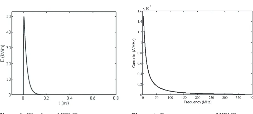
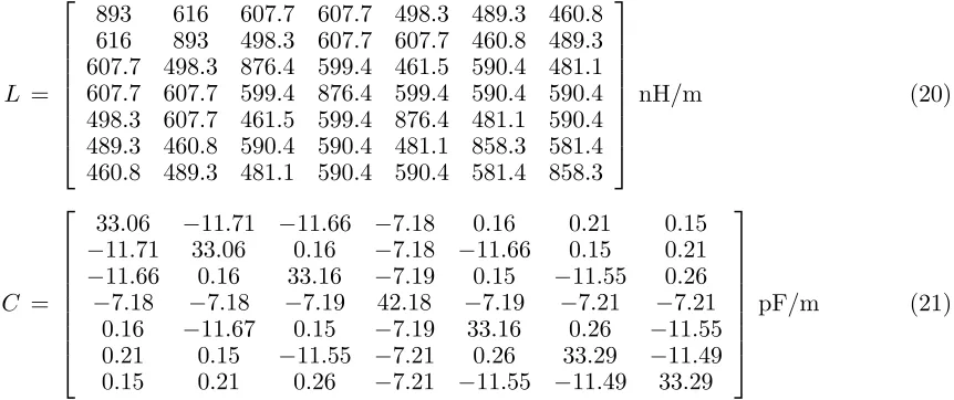
Electric ﬁeld intensity waveform of HEMP in time domain is a double-exponential pulse, as shown in Fig. 3. Fig. 4 reveals frequency spectrum of HEMP.

Figure 3. Waveform of HEMP.

0 50 100 150 200 250 300 350 400

0 0.2 0.4 0.6 0.8 1 1.2 1.4 1.6x 10

-3

Frequency (MHz)

Cu

rr

e

n

ts

(A

/M

Hz

)

Figure 4. Frequency spectrum of HEMP.

3.2. Case of Pure Resistance

There are seven conductors (cables 1–7) to be simpliﬁed and one observed conductor (cable 0) to be monitored just as shown in Fig. 5, and termination loads of complete conductors are presented in Table 1.

0 3 4 5

6 7

Figure 5. Complete cable bundle.

Table 1. The termination loads of complete conductors (unit: Ω).

Conductor 1 2 3 4 5 6 7 0

End 1 50 100 10 k 1 k 500 150 k 1 M 50

End 2 50 10 150 20 M 500 20 15 k 50

(6)

Then complete matrixes of inductance and capacitance of original cable bundle settings are ﬁgured out as Eqs. (20) and (21).

L =

⎡ ⎢ ⎢ ⎢ ⎢ ⎢ ⎢ ⎢ ⎣

893 616 607.7 607.7 498.3 489.3 460.8 616 893 498.3 607.7 607.7 460.8 489.3 607.7 498.3 876.4 599.4 461.5 590.4 481.1 607.7 607.7 599.4 876.4 599.4 590.4 590.4 498.3 607.7 461.5 599.4 876.4 481.1 590.4 489.3 460.8 590.4 590.4 481.1 858.3 581.4 460.8 489.3 481.1 590.4 590.4 581.4 858.3

⎤ ⎥ ⎥ ⎥ ⎥ ⎥ ⎥ ⎥ ⎦

nH/m (20)

C =

⎡ ⎢ ⎢ ⎢ ⎢ ⎢ ⎢ ⎢ ⎣

33.06 −11.71 −11.66 −7.18 0.16 0.21 0.15

−11.71 33.06 0.16 −7.18 −11.66 0.15 0.21

−11.66 0.16 33.16 −7.19 0.15 −11.55 0.26

−7.18 −7.18 −7.19 42.18 −7.19 −7.21 −7.21 0.16 −11.67 0.15 −7.19 33.16 0.26 −11.55 0.21 0.15 −11.55 −7.21 0.26 33.29 −11.49 0.15 0.21 0.26 −7.21 −11.55 −11.49 33.29

⎤ ⎥ ⎥ ⎥ ⎥ ⎥ ⎥ ⎥ ⎦

pF/m (21)

Then, we use ECBM and fast equivalent method to calculate electromagnetic response under HEMP irradiation, respectively.

3.2.1. Original ECBM

By original ECBM in [6, 7], the calculated cable bundle common mode characteristic impedance

Zmc= 175.31 Ω. Then cable decomposition is described as:

Group 1: conductors 1, 2; Group 2: conductors 3, 6; Group 3: conductors 4, 5, 7.

0 3 4 5

6 7

0

G1

G2 G3

dG23

Figure 6. Reduced cable bundle by ECBM.

The model of equivalent cable bundle by ECBM is presented in Fig. 6. Then, according to the theory of ECBM, reduced inductance matrix is as:

Leq =

₇₅₄_.₅ ₅₁₄ ₅₄₅_.₂ 514 728.9 532.5 545.2 532.5 685.7

nH/m (22)

The adjusted cross-section geometry parameters are described in Table 2, and equivalent termination loads are presented in Table 3.

3.2.2. Fast Equivalent Method

Following the fast equivalent algorithm introduced in Section 2, the parameters are calculated. Equivalent cable position is the same as cable 4 because of symmetry of the complete cable bundle settings. According to complete matrix of inductance in Eq. (20) as well as formulas of inductance Eqs. (10) and (15), reduced inductance of equivalent cable Leq = 584.37 nH. By Eq. (16), equivalent

radiusreq= 2.15 mm. Termination loads of equivalent cable are ﬁgured as: End 1 is 30.20 Ω, and End 2

(7)

Table 2. Cross section geometry parameters (unit: mm).

Parameters G1 G2 G3

Radius 1.0 1.0 1.25

Height 22.0 19.1 19.7

Interval d12 = 3.15 d13 = 2.7 d23 = 2.71

FOOTNOTE:dij indicates the interval distance between ith conductor and jth

conductor.

Table 3. Reduced termination loads (unit: Ω).

Conductor G1 G2 G3

End 1 33.33 9376.0 333.22

End 2 8.33 17.65 483.86

3.2.3. Comparison of Two Methods

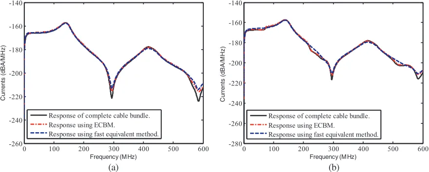
Simulation settings: an inﬁnite metal ground, observed cable 0 is a single conductor of LIFY 0qmm10, and incident direction of excitation source is normal to the cable bundle. The observed cable responses of complete case, reduced by ECBM and fast equivalent method at both cable ends, are presented in Fig. 7.

0 100 200 300 400 500 600

-260 -240 -220 -200 -180 -160 -140

Frequency (M Hz)

C

u

rre

n

ts

(d

B

A

/M

H

z

)

Response of complete cable bundle. Response using ECBM.

Response using fast equivalent method.

0 100 200 300 400 500 600

-280 -260 -240 -220 -200 -180 -160 -140

Frequency (M Hz)

C

u

rre

n

ts

(d

B

A

/M

H

z

)

(a) (b)

Figure 7. Response of observed cable 0 on pure resistance case. (a) End 1. (b) End 2.

As shown in Fig. 7, the response of the proposed method has a little deviation especially at high frequency resonance points. However, the whole trends of three current curves are the same, with good agreement. The statistic results of computation time and memory requirement are displayed in Table 4.

Table 4. Comparison of computation time and memory requirement.

Case of conductors Computation time Acquired memory

The complete cable 2 min 34 sec 60616 kB

ECBM 1 min 20 sec 50916 kB

(8)

From Table 4, we can observe that computation time of fast equivalent method is reduced by 67.5% and memory requirement reduced by 24.8%, compared with the complete cable, while compared to ECBM, computation time is reduced by 37.5% and memory requirement reduced by 10.4%, which veriﬁes the eﬀectiveness of proposed method.

3.3. Case of Hybrid Loads

In hybrid loads case, the original ECBM is not appropriate anymore. Here, we apply GECBM and our fast equivalent method, respectively, and compare with the response of complete cable bundle. The complete cable bundle model is the same as Fig. 5.

The upper cutoﬀ frequency of HEMP is chosen as 300 MHz, total frequency sampling number as 1201, and interval of frequency sampling as 0.25 MHz. Original termination loads and WAV of all termination load impedances are displayed as shown in Table 5.

Table 5. WAV of all termination load impedances.

Conductor 0 1 2 3

Z₁ 50 Ω 50 Ω 100 Ω + 0.1µH 10 kΩ100 pF

|Z1| 50 Ω 50 Ω 109 Ω 379 Ω

Z₂ 50 Ω 10 kΩ 100 Ω10 pF 0.1 Ω + 40 nH + 200 pF

|Z2| 50 Ω 10 kΩ 22.6 Ω 147 Ω

Conductor 4 5 6 7

Z1 0.2 Ω + 20 nH + 100 pF 15 kΩ40 nH20 pF 150 kΩ + 1µH 1 MΩ

|Z1| 289 Ω 44 Ω 150 kΩ 1 MΩ

Z2 20 kΩ200 nH10 pF 500 Ω + 400 nH 750 Ω50 pF 800 Ω + 600 nH

|Z2| 164 Ω 530.8 Ω 45.6 Ω 844 Ω

3.3.1. GECBM

Following GECBM, common mode impedance is asZmc= 177 Ω. Considering modulus of the terminal loads at each end of the cable, the cable groups are:

Group 1: 2; Group 2: 7; Group 3: 1, 5; Group 4: 3, 4, 6.

The reduced model of cable bundle by GECBM is shown in Fig. 8. Cross-section geometry parameters and reduced termination loads are shown in Table 6 and Table 7, respectively.

Table 6. Cross-section geometry parameters (unit: mm).

Parameters G1 G2 G3 G4

Radius 0.50 0.50 1.31 1.26

Height 22.00 18.00 2.00 19.50

Interval d12 = 4.00 d13 = 2.00 d14 = 3.61 d23 = 2.46 d24 = 3.00 d34 = 1.73

FOOTNOTE: dij indicates the interval distance between ith conductor and jth conductor.

3.3.2. Fast Equivalent Method

(9)

Table 7. Reduced termination loads (unit: Ω).

Conductor G1 G2 G3 G4

End 1 109 1 M 23.4 163.8

End 2 22.6 844.0 504.0 28.7

0 3 4 5

6 7

0

G4

G2

Figure 8. Reduced cable bundle by GECBM.

0 100 200 300 400 500 600

-250 -240 -230 -220 -210 -200 -190 -180 -170 -160 -150

Frequency (MHz)

C

u

rre

n

ts

(d

B

A

/M

H

z

)

Response of complete cable bundle. Using GECBM.

Using fast equivalent method.

0 100 200 300 400 500 600

-250 -240 -230 -220 -210 -200 -190 -180 -170 -160 -150

Frequency (MHz)

C

u

rre

n

ts

(d

B

A

/M

H

z

)

Response of complete cable bundle. Using GECBM.

Using fast equivalent method.

(a) (b)

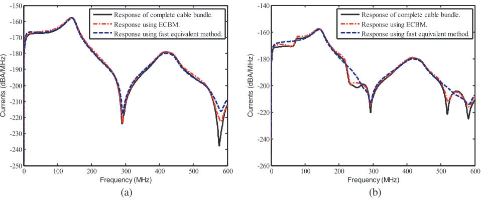
Figure 9. Response of observed cable 0 on hybrid load case. (a) End 1. (b) End 2.

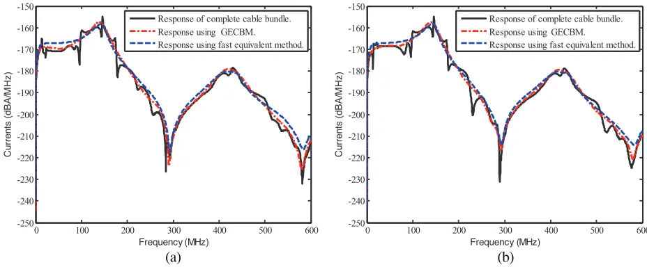
It can be seen that GECBM results have excellent precision, while fast equivalent method combined with WAM also has good agreement generally, other than a little deviation at high frequency resonance points. The statistics results of computation time and memory requirement are displayed in Table 8.

Table 8. Comparison of computation time and memory requirement.

Case of conductors Computation time Acquired memory

The complete cable 3 min 53 sec 56912 kB

GECBM 2 min 20 sec 54408 kB

Fast equivalent method 1 min 19 sec 47056 kB

In terms of computation time and memory requirement, compared with the complete cable, computation time of fast equivalent method combined with WAV is reduced by 66.1% and memory requirement reduced by 17.3%, while compared to GECBM, computation time is reduced by 43.6% and memory requirement reduced by 13.5%.

(10)

GECBM, in spite of slight loss of calculation accuracy at high frequency resonance points. However, coupled energy in cable 0 at high frequency is much smaller than that of other frequency components due to HEMP energy distribution as shown in Fig. 4. Therefore, the discrepancy in high frequency will not have great impact on overall results. Moreover, the proposed equivalent method is easier to perform, and calculation time and memory is signiﬁcantly reduced to meet fast engineering application need.

3.4. Influence of Distance between Observed Cable and Cable Bundle

Finally, the influence of distance between cable 0 and cable bundle is studied to further verify the effectiveness of the fast equivalent method. Here, we defined as the distance between cable 0 and the center of cable bundle, as shown in Fig. 10. Both cases of terminated loads are analyzed in detail.

0 3 4 5

6 7

0

1-7

Figure 10. The distance between cable 0 and cable bundle.

3.4.1. Case of Pure Resistance

In part of Subsections 3.2 and 3.3, the distance d equals 20 mm. Then, we change d from 20 mm to 6 mm with step of 2 mm. In particular, dequaling 6 mm means that the interval of cable 0 and cable 3 is 2 mm, which means that cable 0 is almost a part of the cable bundle. The simulation results are shown as follows, and only part of the results with several distancesd are presented for limit of content. From Fig. 11 to Fig. 13 and together with Fig. 7, we can see that the trends of three curves are always same. However, accuracy of the proposed method is proportional to d. As d decreases, the result of fast method tends to smooth the resonance part of the complete cable bundle curve. Since the fast method is an approximation method at the expense of losing accuracy compared to ECBM,

0 100 200 300 400 500 600

-250 -240 -230 -220 -210 -200 -190 -180 -170 -160 -150

Frequency (MHz)

C

u

rre

n

ts

(d

B

A

/M

H

z

)

0 100 200 300 400 500 600

-280 -260 -240 -220 -200 -180 -160 -140

Frequency (MHz)

C

u

rre

n

ts

(d

B

A

/M

H

z

)

(a) (b)

(11)

0 100 200 300 400 500 600 -250 -240 -230 -220 -210 -200 -190 -180 -170 -160 -150 Frequency( MHz) C u rre n ts (d B A /M H z )

0 100 200 300 400 500 600

-260 -240 -220 -200 -180 -160 -140 Frequency (MHz) C u rre n ts (d B A /M H z )

(a) (b)

Figure 12. Response of observed cable 0 withd= 10 mm. (a) End 1. (b) End 2.

0 100 200 300 400 500 600

-250 -240 -230 -220 -210 -200 -190 -180 -170 -160 -150 Frequency (MHz) C u rr e n ts (d BA/M H z )

0 100 200 300 400 500 600

(a) (b)

while d is smaller, the coupling effect between cable 0 and cable bundle is stronger, and caused error will increase accordingly. If dequals 6 mm, the one equivalent cable model cannot sufficiently represent the cable bundle. While d is not smaller than 10 mm, the model is effective and can yield satisfactory results. The discrepancy of responses of two termination ends is derived from terminated loads.

3.4.2. Case of Hybrid Loads

Similarly, while cable bundle is terminated with arbitrary loads, the inﬂuence of d is considered as well. As shown in Figs. 14–16, as d becomes smaller, more resonances will appear in the curve of the complete cable bundle. Both GECBM and fast method tend to smooth these resonance parts of the curve. So both methods will fail as d is small enough, ford equaling 6 mm as an example. The range of d not smaller than 10 mm is an acceptable work scope.

(12)

0 100 200 300 400 500 600 -250 -240 -230 -220 -210 -200 -190 -180 -170 -160 -150 Frequency (MHz) C u rre n ts (d B A /M H z )

Response of complete cable bundle. Response using GECBM.

0 100 200 300 400 500 600

Response of complete cable bundle. Response using

(a) (b)

GECBM.

0 100 200 300 400 500 600

-250 -240 -230 -220 -210 -200 -190 -180 -170 -160 -150 Frequency (MHz) C u rre n ts (d B A /M H z )

0 100 200 300 400 500 600

(a) (b)

GECBM. GECBM.

0 100 200 300 400 500 600

(a) (b)

GECBM. GECBM.

(13)

4. CONCLUSIONS

This paper proposes a fast equivalent method of cable bundle terminated in arbitrary loads for electromagnetic pulse response modeling. The complex cable bundle can be simpliﬁed into only one cable, which can perform well not only in pure resistance case, but in frequency dependent loads case by weighted average method. The computation time and memory of the proposed method are improved with acceptable equivalent precision compared to ECBM. Numerical simulations of cable response of observed cable keeping a certain distance away from cable bundle by CST software are given to validate the eﬃciency and advantages of the method under illumination of HEMP.

In this paper, the cable electromagnetic response is calculated by MTLN algorithm. When MTLN algorithm is deficient, full wave analysis algorithm is needed to verify the effectiveness of the proposed method. The effectiveness of the method for other applications should be investigated and verified in the future.

REFERENCES

1. Hyun, S., J. Du, and H. Lee, “Analysis of shielding eﬀectiveness of reinforced concrete against high-altitude electromagnetic pulse,”IEEE Transactions on Electromagnetic Compatibility, Vol. 56, No. 6, 1–9, 2014.

2. Song, S. T., H. Jiang, and Y. L. Huang, “Simulation and analysis of HEMP coupling eﬀect on a wire inside an apertured cylindrical shielding cavity,” Applied Computational Electromagnetics Society Journal, Vol. 27, No. 6, 505–515, 2012.

3. Zhou, B., B. Chen, and L. Shi,EMP and EMP Protection, National Defence Industry Press, Beijing, China, 2003.

4. Cai, J., X. Sun, and X. Zhao, “Eﬀects of windows to the electromagnetic environment of a car radiated by high altitude electromagnetic pulse,”2015 IEEE International Conference on Computer and Communications (ICCC), 207–211, Chengdu, 2015.

5. Gu, C., Z. Shao, Z. Li, et al, “Equivalent method for analyzing crosstalk of cable bundles,”Chinese Journal of Radio Science, Vol. 03, 509–514, 2011.

6. Andrieu, G., L. Kon ´E, F. Bocquet, B. D´Emoulin, and J. P. Parmantier, “Multiconductor reduction technique for modeling common-mode currents on cable bundles at high frequency for automotive applications,” IEEE Transactions on Electromagnetic Compatibility, Vol. 50, No. 1, 175–184, Feb. 2008.

7. Andrieu, G., A. Reineix, X. Bunlon, J. P. Parmantier, L. KonÉ, and B. DÉmoulin, “Extension of the “Equivalent cable bundle method” for modeling electromagnetic emissions of complex cable bundles,”IEEE Transactions on Electromagnetic Compatibility, Vol. 51, No. 1, 108–118, Feb. 2009. 8. Andrieu, G., X. Bunlon, L. Kon’e, J. P. Parmantier, B. D’emoulin, and A. Reineix, “The ‘Equivalent cable bundle method’: An efficient multiconductor reduction technique to model industrial cable networks,”New Trends and Developments in Automotive System Engineering, InTech, Manhattan, NY, Jan. 2011.

9. Li, Z., Z. J. Shao, J. Ding, Z. Y. Niu, and C. Q. Gu, “Extension of the “equivalent cable bundle method” for modeling crosstalk of complex cable bundles,”IEEE Transactions on Electromagnetic Compatibility, Vol. 53, No. 4, 1040–1049, Nov. 2011.

10. Liu, L. L., Z. Li, J. Yan, and C. Q. Gu, “Simpliﬁcation method for modeling crosstalk of multicoaxial cable bundles,” Progress In Electromagnetics Research, Vol. 135, 281–296, 2013.

11. Liu, L. L., Z. Li, J. Yan, and C. Q. Gu, “Application of the “equivalent cable bundle method” for modeling crosstalk of complex cable bundles within uniform structure with arbitrary cross-section,”

Progress In Electromagnetics Research, Vol. 141, 135–148, 2013.

(14)

13. Liu, L., Z. Li, M. Cao, and C. Gu, “A generalized equivalent cable bundle method for modeling crosstalk of complex cable bundles with multiple excitations,” 2012 Asia-Pacific Symposium on Electromagnetic Compatibility, 269–272, Singapore, 2012.

14. Andrieu, G., S. Bertuol, X. Bunlon, J. Parmantier, and A. Reineix, “Discussions about automotive application of the ‘equivalent cable bundle method’ in the high frequency domain,”20th Int. Zurich Symposium on EMC Proceedings, Zurich, 2009.