Diagonal Factorization of Integral Equation Matrices via Localizing
Sources and Orthogonally Matched Receivers
Robert J. Adams* and John C. Young
Abstract—A procedure is reported to determine accurate, invertible, block-diagonal factorizations for matrices obtained by discretizing integral equation formulations of electromagnetic interaction problems. The algorithm is based on the combination of localizing source/receiver transformations with orthogonally matched receiver/source transformations. The resulting factorization provides a single, sparse data structure for the system matrix and its inverse, and no approximation is required to convert between the two. Numerical examples illustrate the performance of the factorization for electromagnetic scattering from perfectly conducting elliptical cylinders of different electrical size.
1. INTRODUCTION
The development of efficient simulation tools for electromagnetic radiation, transmission, and scattering problems has been an active area of research for many decades. A relatively recent focus has been the development of sparse, direct solution methods for the linear systems obtained by discretizing time-harmonic integral equation representations of EM interaction problems. Unlike iterative methods, direct methods provide a fixed-cost solution for each excitation. This can provide substantial computational savings relative to iterative methods for problems involving multiple right-hand sides. Sparse direct methods also provide general-purpose preconditioners for fast iterative methods.
Multiple strategies have been used to develop sparse direct solvers, e.g., [1–7]. The set of approaches considered here are based on the use of localizing functions [8–13]. Localization-based direct solvers incorporate source functions having support in individual groups (of an underlying multilevel tree) that localize their scattered fields to the group that contains the source. In one approach, localizing sources have been combined with orthogonally matched receivers to obtain an upper-triangular factorization [10– 13]. In the following, this approach is extended to obtain a data-sparse, block-diagonal representation of the system matrix. The new representation is easily inverted without fill-in or further approximation. Numerical examples of TMz scattering from perfect conductors are used to illustrate the performance of the factorization algorithm. A diagonal factorization algorithm for symmetric matrices is detailed in [14].
2. BACKGROUND
Discretized integral equation formulations of linear, time-harmonic, electromagnetic interaction problem can be represented as a matrix equation,
Zx=Fi. (1)
In this equation, xis an N ×k matrix containing the coefficients (or degrees of freedom, DOF) of the underlying bases used to represent the sources in the integral equation. The integer N is the number
Received 12 December 2016, Accepted 27 March 2017, Scheduled 13 April 2017 * Corresponding author: Robert J. Adams ([email protected]).
of DOF, andk is the number of excitation vectors. Fi is anN ×k matrix determined from samples of
k excitation functions. The system matrix, Z, is determined using a moment method to discretize the underlying integral operator [15].
As described in [12, 13], a multilevel tree is used to organize interactions on the simulation domain. The number of levels in the tree is L, and tree levels are indexed from 1 to L. Level-1 is the coarsest (root) level of the tree, and level-L is the finest level. The level index for a general level is level-l, and individual groups at level-l are indexed as m(l). The level index (l) in m(l) will be suppressed for simplicity when the level is clear from the context. In the following, a multilevel, data-sparse, H2 representation [16] is used to represent Z. The procedure used to construct the H2 representation is discussed in [13].
2.1. Triangular Factorization
Different factorization algorithms can be developed using localizing transformations [8–13]. This section briefly reviews a triangular factorization [10–12]. The proposed diagonal factorization is a modification of this algorithm. In this paper, only non-overlapped localizing functions are used; that is, the support of each localizing function is confined to a single group at a given level of the multilevel tree. (Overlapped localizing functions are necessary for efficient computational performance in 3-D applications [13] and are not considered in this paper.)
The multilevel, triangular factorization obtained using the localizing basis functions is (cf. Equation (27) of [12]),
Z(l+1NN)=PlPHl Z(l+1NN)ΛlΛ−l 1 ≈
P(lL) P(lN) I Z
(LN) l
0 Z(lNN) Λ
(L) l Λ(lN)
−1
, (2)
wherelindicates the tree level. The original system matrix in Eq. (1) is obtained forl=L,Z=Z(LNN+1). The matrices Λl and Pl in (2) are square, permuted block-diagonal matrices (e.g., see Figure 1(b) of [13]). Their diagonal blocks have a dimension equal to the number of remaining DOF in Z(l+1NN)
associated with each level-l group, m(l). The superscripts (L) and (N) are used to indicate matrices associated with localizing and non-localizing sources, respectively. The localizing source DOF are in
Λ(lL), and non-localizing DOF are in Λ(lN); the latter are selected such thatΛ(lN) is orthogonal toΛ(lL), which improves the conditioning ofΛl. The matrix Pl is unitary.
The approximation indicated in Eq. (2) is due to approximate source localization. The localizing source functions inΛ(lL)only localize their scattered fields,Zl(+1NN)Λ(lL), to order-, whereis the desired
accuracy for the factorization. It is noted that in (2) and throughout this paper, all matrices Z(NNl )
and Z(lLN) are represented using an l-level H2 data structure [16]. The procedure used to efficiently
manipulate the H2 data structures to compute the localizing functions in Λ(lL) is discussed in detail in [12, 17]. All other matrices, including Λl and Pl above, and Xl and Yl below, are either block diagonal or permuted block diagonal matrices.
An important property of Eq. (2) is that the submatrixZ(lNL) =P(lN)Z(l+1NN)Λ(lL)≈0 is negligible to order-. This occurs becauseP(lN) is constructed to be orthogonal (to order-) to the fields radiated by the localizing DOF, Z(l+1NN)Λl(L). In this sense, the receiving vectors P(lN) are orthogonally matched
to the localizing sources, Λ(lL). This orthogonal matching provides the upper triangular structure of Eq. (2), which enables the following approximate inverse,
Z−1 =
Z(LNN+1)
−1
≈ΛL ⎡ ⎢
⎣ I −Z
(LN) L
Z(LNN)
−1
0
Z(LNN)
−1
⎤ ⎥
⎦PHL. (3)
3. DIAGONAL FACTORIZATION
The feature of (2) that yields the simple inversion formula (3) is the orthogonal pairing of the receivers in P(lN) and the localizing sources in Λ(lL). In the following, this aspect of (2) is extended to obtain a diagonal factorization for asymmetric matrices. A diagonal factorization algorithm for symmetric matrices is reported in [14].
Begin by defining a right transformation,
Xl=Λl,R, P∗l,R (4)
and a left transformation,
Yl=Λl,L, P∗l,L (5)
where * denotes complex conjugation. In these equations, the sub-matrixΛl,R is the sub-matrixΛ(lL)of Eq. (2), and Pl,L is the sub-matrixP(Nl ). BothΛl,R and Pl,L are obtained analyzing column blocks of
Z(lNN) using the algebraic methods detailed in [12, 17]. The sub-matricesΛl,L andPl,R are obtained by performing the same algebraic analysis on row-blocks ofZl. (It is noted that Xl and Yl are permuted block-diagonal matrices with the same structure as Λl and Pl above.)
The localizing, block-diagonal sub-matricesΛl,LandΛl,Rcan be expressed in terms of their diagonal blocks as
Λl,L = diagλ1l,L, . . . ,λml,L, . . . ,λMl,L (6)
Λl,R = diagλ1l,R, . . . ,λml,R, . . . ,λMl,R (7)
whereλml,Lis the collection of localizing vectors in group-mfor which the operation (λml,L)TZl(m(l),:) is nonzero (to order-) only within columns associated with group-m. (The notation Zl(m(l),:) is used to indicate the rows ofZlassociated with group-mat level-lof the tree.) Similarly,λml,Ris the collection of localizing vectors in group-mfor which the productZl(:, m(l))λml,Ris nonzero only within rows contained by the same group-m at level-l of the tree.
The transformationsXl andYlindicated by Eqs. (4) and (5) provide the following approximation
Zl+1 =Yl−TYTl Zl+1XlX−l 1≈Y−l T
Bl 0
0 Zl
X−l 1, (8)
where the system matrix is obtained whenl=L,Z=ZL+1. The superscript (NN) in Eq. (2) is dropped for convenience in (8) and in the following. The elements of Eq. (8) are,
P∗l,LTZl+1Λl,R ≈ 0, (9)
(Λl,L)T Zl+1P∗l,R ≈ 0, (10)
(Λl,L)TZl+1Λl,R = Bl, (11)
P∗l,LT Zl+1P∗l,R = Zl. (12)
The products (9) and (10) are O(ε) for the same reason that Z(NL) is approximately zero in Eq. (2). Due to localization, the matrixBl is block-diagonal (to order-):
Bl = diagb1l, . . . ,bml , . . . ,bMl . (13)
The diagonal blocks are
3.1. Error Control
Due to approximation, it is possible that the errors in the factorization of Eq. (8) may be larger than the desired tolerance, O(), if the transformations Xl and/or Yl are poorly conditioned. It has been observed that this situation can be avoided by ensuring that the diagonal blocks of the matrix Bl are sufficiently well-conditioned relative to the tolerance.
An SVD of the diagonal blocks ofBl provides,
bml =um(l)σm(l)vHm(l) (15)
where σm(l) = diag(σ1, . . . , σk, . . . , σKm) is the diagonal matrix of singular values, and Km indicates the number of localizing sources in group m(l). Let ¯vm(l) (¯um(l)) denote the columns of vm(l) (um(l)) corresponding to singular values that satisfy
σk> σ1γ, (16)
where
γ = max
1/2, κ−1/2 self
. (17)
In Eq. (17), is the factorization tolerance andκself is the condition number of the self-block of Zl+1 associated with groupm(l) (i.e., the condition number of Zl(m(l), m(l)) ). Finally, let ¯σm(l) denote the diagonal matrix of singular values associated with ¯vm(l) and ¯um(l), and let ¯sm(l) denote the diagonal matrix containing the square root of the singular values such that,
¯
σm(l)= ¯sm(l)¯sm(l) (18) The block-diagonal collection of the ¯vm(l) (¯um(l)) for all level-l groups is denoted ¯vl (¯ul). Similarly, the collection of the ¯sm(l) is denoted ¯sl. Updated versions of Eqs. (4) and (5) that provide better conditioning are thus
¯
Xl=Λ¯l,R, P¯∗l,R (19)
¯
Yl=Λ¯l,L, P¯∗l,L (20)
where ¯Λl,R = Λl,Rv¯l¯s−l 1 and ¯Λl,L =Λl,Lu¯∗l¯sl−1. The diagonal blocks of ¯Pl,R (or ¯Pl,L) are determined from the null-space of the localized fields,Zl+1Λ¯l,R (or ¯ΛTl,LZl+1), in the manner described forP
(N) l of Eq. (2) in [10, 12].
3.2. Multilevel Factorization
The updated version of Eq. (8) obtained using Eqs. (19) and (20) is,
Zl+1 ≈Y¯l−T
I 0 0 Zl
¯
X−l 1. (21)
As shown in the following numerical examples, the error-controlled factorization in Eq. (21) is significantly more accurate than the factorization in Eq. (8). The multilevel approximate inverse associated with Eq. (21) is,
Z−l+11 ≈X¯l
I 0 0 Z−l 1
¯
YlT. (22)
The recursive expansion of the factorization in Eq. (21) is,
Z≈Y¯L−TY¯L−−T1· · ·Y¯3−TY¯2−T
I 0 0 Z2
¯
X2−1X¯−31· · ·X¯L−−11X¯−L1, (23)
and the recursive expansion of Eq. (22) is
Z−1 ≈X¯LX¯L−1· · ·X¯3X¯2
I 0
0 Z−21
¯
From Eqs. (23) and (24) it is observed that, in addition to providing a block-diagonal inverse approximation, the diagonal factorization in Eq. (21) also provides a block-diagonal representation ofZ
(each ¯Xl and ¯Yl is a block-diagonal matrix at level-l, and Z2 is a square matrix with dimension equal to the number of remaining, non-localized DOF). Note that Zand Z−1 have identical block-diagonal structures. Thus, once the diagonal representation in Eq. (23) is determined, the inverse Eq. (24) can be obtained without additional approximation or fill-in. In this sense, Eq. (23) provides a single, explicit, data-sparse representation of both the system matrix, Z, and its inverse, Z−1. Although the triangular factorization in Eq. (2) can be inverted via Eq. (3), the inverse requires back-substitution and application of Z(lLN) which is stored as an l-level H2 data structure, at each level of the solution process. For this reason, when using Eq. (3), the memory required by the factorization exceeds the memory used by the initial H2 representation of Z, and the solve process is slowed by the need to apply an l-level H2 data structure at each level of the solve when applyingZ(lLN).
In contrast, using the inverse Eq. (24), it is not necessary to store any off-diagonal data or perform any back-substitution during the solution process. As shown below, the memory required by the diagonal representation in Eq. (24) is actually less than that used by the initial H2 representation in some cases.
3.3. Integrated Factor and Solve (IFS)
An advantage of the diagonal representation in Eq. (24) is that, if the excitation Fi is known a priori, an integrated factor and solve (IFS) can be used to reduce the overall memory requirement of the sparse direct solver.
The IFS procedure proceeds as follows. At each level of the factorization, ¯Yl can be applied to the right-hand side vectors, Fi, as indicated by Eq. (24) and then deallocated. Similarly, at each level the localizing submatrix of ¯Xl, ¯Λl,R, can be applied and then deallocated. The blocks ¯P∗l,R are the only blocks of the diagonal factorization retained throughout the entire IFS process. Once the factorization is completed, the blockZ2 is factored and applied to the right-hand side vector(s), after which the ¯P∗l,R are finally applied, proceeding from coarse to fine levels of the tree, to determine the solution vectors,
x.
4. NUMERICAL RESULTS
To illustrate the numerical properties of the diagonal factorization, consider the problem of TMz scattering from perfectly conducting elliptical cylinders. The magnetic field integral equation (MFIE) is used to formulate the problem. The matrix equation (1) is obtained from the MFIE using a point-matching moment method with pulse basis functions [15] for the case of scattering from a pair of ellipses separated by 0.1λ, each with an axial ratio of 4. The major axis,D, of the ellipses varies between 12λ and 1536λ. The scatterer configuration forD= 1536λis shown in Figure 1. In all cases considered, more than ten basis functions are used per linear wavelength. Similar numerical experiments are reported for symmetric and asymmetric matrices in [14].
The factorization algorithm outlined above relies on the determination of the localizing DOF used to define the blocks Λl,R and Λl,L. As discussed elsewhere [12, 13], this is accomplished by first building a data-sparse H2 representation of Z [16]. The methods used to efficiently manipulate the H2 representation to determine the submatrices Λl,L, Λl,R, Pl,L, and Pl,R of ¯Xl and ¯Yl are detailed in [12, 17]. When the error control procedure is used, the modification indicated by Eq. (15) through Eq. (20) is used to replace Xl and Yl by ¯Xl and ¯Yl. In the following examples, the initial H2 representation of Z is constructed using a tolerance of 1E-6; the subsequent diagonal factorization is performed using a tolerance of 1E-5.
Tables 1 and 2 report relative RMS matrix errors in the H2 data structure and the diagonal factorization. Table 1 reports errors for a fixedD= 12λ;N is increased by increasing the density of the discretization per wavelength. Table 2 reports the matrix errors for the cases of a fixed discretization density;N is increased by increasing the electrical sizes of the ellipses.
Figure 1. Two-ellipse scattering configuration when D = 1536λ (N = 135112). The ellipses are separated by 0.1λat their point of closest proximity.
Figure 2. Memory used by H2 representation, diagonal factorization and integrated factor/solve (IFS) procedure for fixed D = 12λ and increasing discretization density. Also shown are O(N) and O(N2) reference lines.
factorization errors occur when the error control strategy is not employed. For this reason, the error control method outlined above is used in all remaining examples.
Figure 2 displays the memory used for the H2 representation, for the factorization, and for the integrated factor/solve (IFS) procedure for the same fixed major axis cases considered in Table 1. It is observed that the memory requirements increase approximately linearly. Furthermore, the diagonal factorization requires less memory than the H2 representation for all but the smallest case (N = 1056). This suggests that for such cases it may be advantageous to develop a method to directly construct the diagonal representation in Eq. (23) rather than first building the H2 structure as was done here. Finally, it is observed that the peak memory required by the IFS procedure does not notably exceed the peak memory required by the initial H2 data structure for these cases.
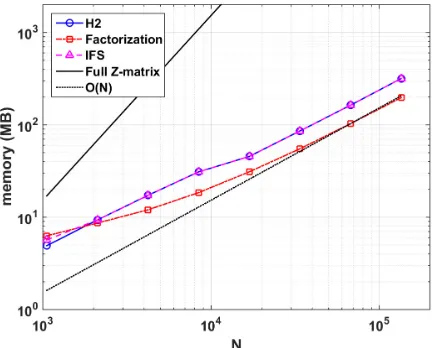
Figure 3 reports the memory requirements when the discretization density is fixed and the major axis, D, increases (cf. Table 2). In these cases, the memory requirements all increase approximately as
Figure 3. Memory used by H2 representation, diagonal factorization, and IFS for fixed discretization density and increasing major axis length. Also shown areO(N1.5) and O(N2) reference lines.
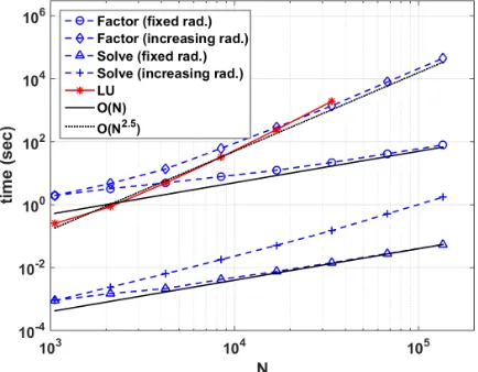
Figure 4. Diagonal factorization and solve times for cases of increasing discretization density with fixed D= 12λ, and for cases of fixed discretization density with increasing D. The performance of an optimized LU factorization is also shown.
increase caused by the direct solver only becomes notable for values ofD larger than about 100λ. Finally, Figure 4 indicates the time used to perform the factorization for the cases in Tables 1 and 2. (All computations were performed on an Intel Xeon X5450 3 GHz Quad-Core Processor.) The figure also shows the time required to solve for a single right-hand side vector given the completed diagonal factorization. In the case of a fixed electrical size and increasing discretization density, the factorization and solution times scale approximately linearly, and the diagonal factorization substantially outperforms LU factorization. However, in the case of a fixed discretization density with increasing D, the factorization does not begin to outperform LU factorization untilN exceeds about 16000.
4.1. Other Formulations
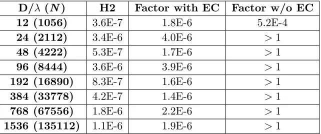
Table 1. Relative RMS errors in Zof (1) using H2 representation and the diagonal factorization (23) with and without error control (EC) procedure. The electrical size is fixed atD= 12λandN is increased by increasing the discretization density. Values >1 indicate that the error exceeds 100 percent. The number of quad-tree levels varies from L= 4 (N = 1056) to L= 11 (N = 135112).
D/λ(N) H2 Factor with EC Factor w/o EC 12 (1056) 3.6E-7 1.8E-6 >1
12 (2112) 9.8E-6 9.8E-6 >1
12 (4222) 3.0E-7 1.6E-6 >1
12 (8444) 2.9E-7 1.4E-6 >1
12 (16890) 2.6E-7 1.3E-6 0.956
12 (33778) 2.5E-7 1.5E-6 0.664
12 (67556) 2.9E-7 1.2E-6 0.477
12 (135112) 2.8E-7 1.3E-6 0.412
Table 2. Same as Table 1 but with increasing electrical size (D) and fixed discretization density.
D/λ(N) H2 Factor with EC Factor w/o EC 12 (1056) 3.6E-7 1.8E-6 5.2E-4
24 (2112) 3.4E-6 4.0E-6 >1
48 (4222) 5.3E-7 1.7E-6 >1
96 (8444) 3.6E-6 3.9E-6 >1
192 (16890) 8.3E-7 1.6E-6 >1
384 (33778) 4.2E-7 1.4E-6 >1
768 (67556) 1.8E-6 2.2E-6 >1
1536 (135112) 1.1E-6 1.9E-6 >1
when the EFIE is used to solve the problems reported herein. This was previously observed in [13] for the EFIE and is due to the well-known ill-conditioning of the EFIE. Fortunately, better conditioned formulations are available, including the augmented EFIE [18, 19]. It has previously been shown that the computational complexity of the factorization (2) is O(NlogN) or better for an augmented EFIE formulation in three dimensions [20]. The application of the new, diagonal factorization to such formulations will be a subject of future investigation.
5. SUMMARY
A diagonal, data-sparse factorization strategy for asymmetric integral equation matrices has been detailed, and a computationally efficient error control strategy has been proposed. The factorization provides a single, sparse data structure for both the system matrix (23) and its inverse (24). There is no fill-in or additional approximation required to convert between the diagonal representations of Z
and Z−1. Due to the diagonal nature of the representation, the solution procedure used to determine x
from Fi involves only explicit matrix multiplication.
electrical size is increased, the diagonal factorization generally uses more memory than the initial H2 representation of Z. However, the additional memory required by the diagonal factorization can be reduced using an integrated factor/solve (IFS) procedure.
For three-dimensional surface integral equation applications with non-oscillatory kernels, the computational complexity of the algorithm reported here is limited to O(N1.5) due to the use of non-overlapped localizing functions [11, 12]. However, the factorization algorithm admits a straightforward incorporation of the overlapped functions defined in [13]. These functions have been observed to yield factorization complexities that scale asO(NlogN) or better for surface integral equations in 3-D using the triangular factorization of (2) [13, 20]. The incorporation of overlapped localizing functions within the diagonal factorization outlined here will be a subject of future investigation.
ACKNOWLEDGMENT
The authors gratefully acknowledge support from the Office of Naval Research (N00014-16-1-3066) and the Kentucky Science and Engineering Foundation (KSEF-148-502-16-393).
REFERENCES
1. Gope, D., I. Chowdhury, and V. Jandhyala, “DiMES: Multilevel fast direct solver based on multipole expansions for parasitic extraction of massively coupled 3D microelectronic structures,”
42nd Design Automation Conference, 159–162, 2005.
2. Shaeffer, J., “Direct solve of electrically large integral equations for problems sizes to 1 M unknowns,”IEEE Transactions on Antennas and Propagation, Vol. 56, 2306–2313, 2008.
3. Jiao, D. and W. Chai, “An H2-matrix-based integral-equation solver of reduced complexity and controlled accuracy for solving electrodynamic problems,” IEEE Transactions on Antennas and Propagation, Vol. 57, 3147–3159, 2009.
4. Heldring, A., J. M. Rius, J. M. Tamayo, J. Parron, and E. Ubeda, “Multiscale compressed block decomposition for fast direct solution of method of moments linear system,” IEEE Transactions on Antennas and Propagation, Vol. 59, 526–536, 2011.
5. Wei, J.-G., Z. Peng, and J. F. Lee, “A fast direct matrix solver for surface integral equation methods for electromagnetic wave scattering from non-penetrable targets,”Radio Science, Vol. 47, 1–9, 2012. 6. Brick, Y., V. Lomakin, and A. Boag, “Fast direct solver for essentially convex scatterers using multilevel non-uniform grids,” IEEE Transactions on Antennas and Propagation, Vol. 62, 4314– 4324, 2015.
7. Zhang, Y. L., X. Chen, C. Fei, Z. Li, and C. Gu, “Fast direct solution of composite conducting-dielectric arrays using Sherman-Morrison-Woodbury algorithm,” Progress In Electromagnetics Research M, Vol. 49, 203–209, 2016.
8. Martinsson, P. G. and V. Rokhlin, “A fast direct solver for boundary integral equations in two dimensions,”Journal of Computational Physics, Vol. 205, 1–23, 2005.
9. Adams, R. J., A. Zhu, and F. X. Canning, “Efficient solution of integral equations in a localizing basis,” Journal of Electromagnetic Waves and Applications, Vol. 19, No. 12, 1583–1594, 2005. 10. Zhu, A., R. J. Adams, F. X. Canning, and S. D. Gedney, “Schur factorization of the impedance
matrix in a localizing basis,” Journal of Electromagnetic Waves and Applications, Vol. 20, No. 3, 351–362, 2006.
11. Adams, R. J., A. Zhu, and F. X. Canning, “Sparse factorization of the TMz impedance matrix in an overlapped localizing basis,” Progress In Electromagnetics Research, Vol. 61, 291–322, 2006. 12. Adams, R. J., Y. Xu, X. Xu, J. S. Choi, S. D. Gedney, and F. X. Canning, “Modular fast direct
electromagnetic analysis using local-global solution modes,”IEEE Transactions on Antennas and Propagation, Vol. 56, 2427–2441, Aug. 2008.
14. Adams, R. J. and J. C. Young, “A diagonal factorization for integral equation matrices,”
2016 International Conference on Electromagnetics in Advanced Applications (ICEAA), 812–815, September 19–23, 2016.
15. Peterson, A. F., S. L. Ray, and R. Mittra, Computational Methods for Electromagnetics, IEEE Press, Piscataway, NJ, 1998.
16. Hackbusch, W. and S. Borm, “H2-matrix approximation of integral operators by interpolation,”
Applied Numerical Mathematics, Vol. 43, 129–143, 2002.
17. Xu, Y., X. Xu, and R. J. Adams, “A sparse factorization for fast computation of localizing modes,”
IEEE Transactions on Antennas and Propagation, Vol. 58, 3044–3049, 2010.
18. Qian, Z. G. and W. C. Chew, “An augmented electric field integral equation for highspeed interconnect analysis,” Microwave and Optical Technology Letters, Vol. 50, 2658–2662, October 2008.
19. Qian, Z. G. and W. C. Chew, “Enhanced A-EFIE with perturbation method,”IEEE Transactions on Antennas and Propagation, Vol. 58, 3256–3264, October 2010.