Extracting Surface Macro Basis Functions from Low-Rank Scattering Operators with the ACA Algorithm

Extracting Surface Macro Basis Functions from Low-Rank Scattering

Operators with the ACA Algorithm

Vito Lancellotti*

Abstract—The Adaptive Cross Approximation (ACA) algorithm has been used to compress the rank-deficient sub-blocks of the matrices that arise in the numerical solution of integral equations (IEs) with the Method of Moments. In the context of the linear embedding via Green’s operator (LEGO) method — a domain decomposition technique based on IEs — an electromagnetic problem is modelled by combining “bricks” in turn described by scattering operators which, in many situations, are singular. As a result, macro basis functions defined on the boundary of a brick can be generated by applying the ACA to a scattering operator. Said functions allow compressing the weak form of the LEGO functional equations which then use up less computer memory and are faster to invert.

1. INTRODUCTION

Scattering and radiation problems in electromagnetics have been formulated in terms of integral equations (IEs) for decades now [1, 2]. Among the reasons that tip the scale in favor of IEs, as opposed to the direct solution of Maxwell’s differential equations, we recall the following two: 1) Sommerfeld’s radiation conditions come naturally incorporated in the operators, and 2) the unknowns of the problem (oft-times equivalent surface or volume current densities) are confined to comparatively small regions of space. Then again, when IEs are solved through the Method of Moments (MoM) [2], they give rise to fully populated matrices, whereas the matrices arising from differential (local) operators are sparse and as such require less time for filling and less computer memory for storage [3]. As a consequence, in order to solve ever larger and more complex problems with IEs, special techniques have been devised to handle large and full matrices. Broadly speaking, researchers have pursued three strategies:

a) Improving the conditioning of the matrix so that it can then be inverted by means of iterative solvers which converge to the solution in an acceptable number of steps.

b) Compressing or sparsifying the matrix so as to reduce the memory occupation and speed up the matrix-vector multiplications for subsequent iterative solution.

c) Dividing the original problem into “smaller” parts amenable to being characterized separately at first, in an attempt to reduce the size of the matrix and to make the inversion thereof feasible with direct solvers.

The first strategy has stimulated research into matrix preconditioning and regularization of the operators (e.g., [4–6]). Clustering techniques, such as the Fast Multiple Method [7] and the H -matrices [8], fall into the second category. The third approach (actually dating as far back as the fifties with the seminal work on diakoptics by Kron [9]) has produced the so-called domain decomposition methods (DDMs) (e.g., [10–15]) which, like as not, are applied in tandem with ad hoc entire-domain basis functions [16–20].

Received 28 April 2016, Accepted 9 July 2016, Scheduled 15 July 2016 * Corresponding author: Vito Lancellotti (v.lancellotti@tue.nl).

Accordingly, in this paper we discuss the generation and the properties of specialized surface macro basis functions for the linear embedding via Green’s operator (LEGO) method, which holds a place in the third group of techniques recalled above. LEGO was developed for 2-D electromagnetic (EM) scattering [21], but the method has been gradually extended to formulate and solve diverse 3-D scattering and radiation problems from aggregate of objects and antennas [20, 22–24].

In line with the philosophy of DDMs, an EM problem is formulated in LEGO by separating the structure into parts which are enclosed within EM “bricks”. The EM behavior of a brick is described by means of a scattering operator, and the EM interactions between two or more bricks and, if present, an antenna are accounted for through suitable transfer operators. Under certain conditions (discussed further on in Section 2.3) the scattering operators may be singular, and this occurrence — far from being an issue — can in fact be exploited to facilitate the solution with the MoM [20, 24, 25]. This goal was achieved in [20] by using the eigenvectors of the scattering operator as a set of macro basis functions (dubbedeigencurrents) over the surface of a brick, and the approach was called eigencurrents expansion method (EEM). It was shown that the response of a brick consists of the eigencurrents weighted with the corresponding eigenvalues. Since the latter decay very fast and, owing to the singular nature of the scattering operator, are mostly null, only the eigencurrents associated with the first few (larger) eigenvalues must be retained in representing the behavior of a brick. Moreover, an approximated criterion was discovered [25] that allows predicting and controlling the accuracy of the EEM in practical cases of interest — which renders the eigencurrents all the more attractive. On the downside, the spectral decomposition of the scattering operator can be time consuming.

Recently, it was realized that the Adaptive Cross Approximation (ACA) [26] can be employed to construct excitation-free macro basis functions over the surface of a brick that afford the same level of accuracy as the eigencurrents [27, 28]. Moreover, carrying out the ACA of the scattering operator is far faster than determining the eigencurrents.

In computational electromagnetics the ACA has been proposed for the fast calculation and compression of the rank-deficient off-diagonal blocks of the matrix that arises from the discretization of the electric field integral equation (EFIE) [29, 30], and for the fast derivation of fields in the far region of a source [31]. Thus, the application of the ACA for the extraction of macro basis functions from low-rank operators in LEGO is new, and constitutes the main contribution of this work. What’s more, this approach is fairly general and capable of extension to other DDMs similarly based on equivalence separation surfaces, such as the Equivalence Principle Algorithm [10, 14] and the Generalized Surface Integral Equation method [13], because the scattering operators therein can be rank-deficient as well.

The remainder of the paper is organized as follows. First, the formulation of scattering and radiation problems with LEGO is recalled in Section 2.1, whereas the weak form of the equations is outlined in Section 2.2. The conditions for the scattering operators to be low-rank are discussed in Section 2.3. Next, the generation of the new macro basis functions with the ACA is outlined in Section 3.1, the compression of the equations is elucidated in Section 3.2, and the efficient calculation of the relevant operators is described in Section 3.3. Finally, in Section 4 we elaborate on the properties of the proposed macro basis functions by considering a radiation problem. A time dependence for sources and fields in the form of exp(jωt) is assumed and suppressed throughout.

2. LINEAR EMBEDDING VIA GREEN’S OPERATORS

To put the macro basis functions (Section 3) in context, hereinbelow we list the functional equations of LEGO applied to a set of ND bodies [20] and, optionally, an antenna made of perfect electric conductor (PEC) [24]. The bodies — each one included in a LEGO brick — and the antenna exist in a homogeneous background medium (labelled with➀). We denote the kth brick with D_k,k= 1, . . . , ND,

and the boundary thereof with ∂Dk.

2.1. LEGO Functional Equations for Scattering and Radiation Problems

The scattering fromND bodies, which are illuminated by an impinging EM wave produced by external sources, is governed by the set ofND coupled functional equations [20]

where

• Idenotes a suitable identity operator on the composite surface∪N_k=1D∂Dk;

• Skk is the scattering operator [20, Eq. (11)] of the EM brickDk;

• T is the total transfer operator [24, Eq. (12)], i.e., an abstract ND ×ND matrix containing the

transfer operatorsT_kn [20, Eq. (15)] between any two bricksD_nand D_k,n=k;

• qs,i are abstract column vectors containing q_ks,i, the equivalent scattered and incident current densities on the boundary∂Dk, namely,

q_ks,i:=

Js,i_k√η1 −Ms,i_k/√η1

, η1 := (μ1/ε1)1/2, (2)

withJs,i_k and Ms,i_k electric and magnetic surface currents.

The radiation from a PEC antenna in the presence of ND objects is governed by the functional

equations [24]

η1(LANT+PAOSTOA)JA=−

Eg_Atan, qs=√η1STOAJA, (3)

with

S:= (I−diag{S_kk}T)−1diag{S_kk}, (4)

where

• LANT denotes the standard EFIE operator within a normalization factor [24, Eq. (16)];

• PAO and TOA are abstract 1×ND and ND ×1 matrices of operators (PAO)k and (TOA)k [24,

Appendix C].

• JAis the equivalent electric current density flowing on the antenna surface SA;

• Eg_Ais the impressed field provided by the generator in the delta-gap model of the antenna port [24];

• qs is the same abstract vector as in (1) and defined with the aid of Eq. (2).

2.2. Baseline Method of Moments

A weak form of Eqs. (1)–(4) follows by applying the MoM in the form of Galerkin [1] with surface and volume sub-sectional divergence-conforming basis functions, as prescribed by the nature of the objects embedded in the bricks. In particular, to expand the currents qs,i_k we model ∂Dk with a triangular

tessellation on which we define a set of 2NF Rao-Wilton-Glisson (RWG) basis functions [20]. If an

antenna is also present, then we model SA by means of a 3-D triangular-faceted mesh on which we

introduce NA RWG basis functions to expressJA [24].

The calculation of the operatorsT_kn, (TOA)_k and (PAO)_k entails the numerical solution of surface

IEs on appropriate pairs of surfaces [20, 24], whereas the procedure followed to derive the algebraic counterpart ofS_kkdepends on the EM properties of the object enclosed inD_k. For instance, if the body is a PEC or is comprised of a penetrable isotropic homogeneous medium, we formulate the internal scattering problem by means of suitable surface IEs [20] involving the equivalent surface current densities on the object. For the numerical solution with the MoM we useNO RWG functions associated with the

triangular mesh that models the surface of the body. Alternatively, if the object is penetrable and either inhomogeneous or anisotropic or both, then we resort to a volume IE for the calculation of the electric or magnetic flux density in the region occupied by the body [23]. To this purpose, we model the object by means of a tetrahedral mesh, and we introduceNO Schaubert-Wilton-Glisson (SWG) functions.

In the end, applying the MoM provides us with the algebraic counterparts of the operators involved in Eqs. (1), (3)–(4), namely, [Skk], [Tkn], [TOAk], [PAOk] and [LANT]. Specifically, [Skk], [Tkn] are square

matrices with size 2NF ×2NF, [TOAk], [PAOk] have size 2NF×NAandNA×2NF, and [LANT] has rank

NA. With these intermediate results it is straightforward to write the weak form of Eqs. (1), (3)–(4), viz.,

([I]−blkdiag{[Skk]}[T]) [qs] = blkdiag{[Skk]}qi, (5)

η1([LANT] + [PAO] [S] [TOA]) [JA] =−EAg

, [qs] =√η1[S] [TOA] [JA], (6) [S] := ([I]−blkdiag{[Skk]}[T])−1blkdiag{[Skk]}, (7)

• [I] is the identity matrix of size 2NFND×2NFND;

• [qs,i] are column vectors with ND block entries [qs,i_k] as defined in [24, Eq. (42)];

• [JA] is a column vector containing theNA expansion coefficients ofJA.

2.3. The Low-Rank Nature of [Skk]

The algebraic scattering operator [Skk] is a singular matrix [20, 23, 25], whenever the following two

conditions are simultaneously met:

(i) The boundary∂Dk of the brick sits at some distance away from the surface of the body.

(ii) The host medium (➁) which pads a brick’s interior is the same as the background medium (➀).

This circumstance is manifest from the explicit expressions for [Skk] given in [20, Eq. (21)] or [23,

Eq. (20)] in case 2NF > NO, that is, the number of unknowns on∂Dkexceeds the number of unknowns

on the surface or in the volume of the object inside D_k. And yet, the low-rank nature of [Skk] is a

more fundamental characteristic related to the fact that the scattered tangential fields over∂Dk possess

fewer degrees of freedom (DoF) than the corresponding quantities over the surface of the object, and this property is somewhat independent of the specific discretization adopted for Eq. (1). In practice, the rank of [Skk] decreases as the distance between ∂Dk and the object is increased [25]. By contrast,

if medium ➁is different than medium➀, then the boundary∂Dk constitutes a material interface, and

[Skk] is full-rank [22]. This happens because the “observation” surface ∂Dk and the surface of the

“obstacle” coincide, and hence no reduction of DoF occurs.

In this regard, an insightful comparison can be drawn to the generalized scattering matrix (GSM) of an obstacle, e.g., an iris, in a classic hollow-pipe waveguide [32]. As is well known, the number of guided modes (i.e., DoF) that concur to define the GSM of the discontinuity decreases as the reference planes are set farther away along the waveguide on either side of the obstacle. In particular, the choice of reference planes flush with the discontinuity corresponds with the aforesaid situation where∂Dk is a

material interface.

3. THE NEW SET OF SURFACE MACRO BASIS FUNCTIONS 3.1. Adaptive cross Approximation of [S_kk]

Having recognized that, under the hypotheses of Section 2.3, [Skk] may be low-rank, we apply the discrete version of the ACA algorithm [26, 29] to [Skk] in order to derive a set of macro basis functions

with support over ∂Dk. Afterrk steps of the algorithm have been completed, we can write

[Skk]≈

S_kk(rk)

:= [Ukk] [Vkk], (8)

where [Ukk] and [Vkk] have size 2NF ×rk and rk×2NF, respectively, andrk denotes the effective rank

of [Skk]. The ACA is stopped as soon as the condition (adapted from [29, Section IV-C])

ε(_kkrk):=

U_kk(rk) 2

V_kk(rk) 2

S_kk(rk)

F

≤t, (9)

is fulfilled, where

• ε(_kkrk) is the approximation error of [Skk] at steprk;

• U_kk(rk)

(

V_kk(rk)

) is the rkth column (row) of [Ukk] ([Vkk]) computed at steprk;

• S_kk(rk)

is the approximation of [Skk] attained at step rk;

Storing [Ukk] and [Vkk] separately requires 4NFrk complex memory locations as opposed to the (2NF)2 locations needed for [Skk], though saving memory is not the main reason for carrying out the

ACA of the scattering operator. Furthermore, in keeping with the ACA — which does not require the full calculation of the matrix to be factorized — we employ the approximate scattering operator

S_kk(rk)

in Eq. (9), even though [Skk] is known when the algorithm is started. Finally, the time taken

to achieve the factorization (8) scales as O(4NFr_k2) (see discussion in [29, Section IV-C]). This number ought to be contrasted with O((2NF)3), which is the asymptotic operation count for the calculation of all eigenvectors and eigenvalues of [Skk] [20] through reduction to Hessenberg form and subsequent QR factorization [33, Chapter 11].

Next, we insert the rightmost hand side of Eq. (8) into Eq. (5), and after a few manipulations we obtain

[qs] = blkdiag{[Ukk]}blkdiag{[Vkk]} qi+ [T] [qs]= blkdiag{[Ukk]}[c], (10)

where [c] is a column vector of_krk coefficients yet to be determined. Nevertheless, Eq. (10) suggests

that we can express the unknown vector [qs_k] as a linear combination of the columns of [Ukk]. The latter,

when associated with the underlying set of 2NF RWG functions on∂Dk (see Section 2.2), define

entire-domain macro basis functions over ∂Dk, whereby Eq. (10) constitutes a basis change. More important, since we expect thatrk2NF, Eq. (10) enables compressing Eq. (5) and computing [S] efficiently for subsequent usage in Eq. (6).

3.2. Change of Basis and Compression To take advantage of Eq. (10) in practice, we let

[U] := blkdiag{[Ukk]}, [qs] := [U] [˜qs], (11) [V] := blkdiag{[Vkk]}, [˜qi] := [V] [qi], (12)

where the column vectors [˜qs] and [˜qi] contain the _krk expansion coefficients in the reduced basis. By substituting Eq. (8) into Eq. (5) again and making use of Eqs. (11) and (12) we arrive at

[U] ([I]−[V] [T] [U]) [˜qs] = [U] [˜qi], (13) where [I] is the identity matrix of rank _krk. The columns of [Ukk] are not orthogonal in general,

but surely they are linearly independent by construction [29]. Hence, we can left-multiply both sides of Eq. (13) first by [U]H and then by ([U]H[U])−1 (where the superscript H indicates the Hermitian transpose) to obtain the reduced system [27]

([I]−[V] [T] [U]) [˜qs] = [˜qi], (14) whose rank is_krk or, when the bodies and the bricks are identical, NDr1. The inverse of the system

matrix in Eq. (14) constitutes the deflated analogue of the total algebraic scattering operator in Eq. (7) that is,

[ ˜S] := ([I]−[V] [T] [U])−1, (15) or, in other words, the matrix [S] expressed in the vector spaces spanned by the columns of [U] and the rows of [V]. Thus, on account of Eqs. (11), (12) and (15) we find the expression

[S] := [U] ([I]−[V] [T] [U])−1[V], (16) which provides us with an efficient way to compute [S] while shunning the direct solution of the possibly large system in Eq. (5). Finally, Eq. (16) allows writing the algebraic operator appearing in the first of Eq. (6) as follows

3.3. Efficient Calculation of the Algebraic Operators

In spite of the compression that the vector basis [Ukk] can afford, we must regard Eq. (16) as a formal

expression, because the actual calculation and storage of [S] may be, in fact, computationally intensive all the same. But then, determining [S] explicitly is hardly necessary; rather, we just have to organize the matrix-vector and matrix-matrix multiplications judiciously, so as to handle relatively small algebraic operators at any step of the numerical solution procedure. This goal is accomplished as follows:

• To fill [V] [T] [U] in (14), we compute and store the off-diagonal blocks [Vkk] [Tkn] [Unn] and

[Vnn] [Tnk] [Ukk] by examining two bricks at a time.

• To obtain the scattered current coefficients [qs], we solve (14), and then apply (11).

• To build [PAO] [U] and [V] [TOA] in (17), we compute and store the matrices [PAOk] [Ukk] and

[Vkk] [TOAk] by considering the antenna and one brick at a time.

• To compute [PAO] [S] [TOA] in (17) we solve the multiple-right-hand-side system

([I]−[V] [T] [U]) [X] = [V] [TOA], (18) and then multiply the result by [PAO] [U].

• To compute [qs] when an external antenna is present, we use [X] from Eq. (18) in the second of Eq. (16) and apply Eq. (11) again.

4. PROPERTIES OF THE ACA BASIS

The compression of Eqs. (5)–(7) described in Sections 3.1 and 3.2 is independent of the calculation of [Skk], [Tkn] and like operators. Since the overall correctness of the latter was already validated

in [20, 23, 24], here we concern ourselves with the properties of the change of basis represented by Eqs. (11) and (12). Besides, the application of the ACA macro basis functions to EM scattering problems involving PEC objects and penetrable isotropic and anisotropic bodies was considered in [27, 28], where the solutions (scattered currents [q_ks] and radar cross section) were compared to those obtained by compressing the LEGO equations with the eigencurrents [20, 23], that is, the eigenvectors of [Skk]. While

the ACA macro basis functions are equivalent to the eigencurrents in every respect, the generation of the former takes far less time than the spectral decomposition of [Skk].

0 0.02

0.04 0.06 0.08

0 0.02 0.04 0.06 0.08 5

10 x 10 3

z [m]

x [m] y [m]

Antenna port

0 0.02

0.04 0.06 0.08

0 0.02 0.04 0.06 0.08 5

10 x 10 3

x [m] y [m]

z [m]

(a) (b)

Figure 1. Simple radiation problem: (a) A strip-dipole in the presence of four square loops; (b) Corresponding LEGO model withND = 4 cuboidal bricks.

To further support these statements, we employ the modified EFIE in Eq. (6) for the solution of a simple radiation problem involving a center-fed PEC strip-dipole which is symmetrically placed above four infinitely-thin PEC square loops in free space, as pictured in Fig. 1(a). The dipole (designed to resonate at around the frequency f = 2.45 GHz when operated in isolation) is 6 cm long and 0.2 cm wide. The inner (outer) side of the loops is 2.8 (3.2) cm long, and the loops (whose electric length is about 1λ0 at f = 2.45 GHz) are arranged in a planar square lattice with period of 4 cm; the distance between the dipole and the plane of the loops is 1 cm. The LEGO model of the structure comprises

0.4 0.45 0.5 0.55 0.6 100

50 0 50 100 150 200 250 300

d/ 0

Z

[

Ω]

t= 10 -1

t= 10-2

t= 10 -3

imag real

0.4 0.45 0.5 0.55 0.6

100 50 0 50 100 150 200 250 300

Z

[

EE M,NC= 5 0

AC A,t= 10 -3

imag real

λ d/ λ0

Ω]

(a) (b)

Figure 2. Input impedance of the antenna system in Fig. 1 as a function of the electric length of the strip-dipole: (a) Convergence with increasing number of ACA macro basis functions; (b) Comparison with the results obtained through the eigencurrents expansion method (EEM) [24].

a brick are 4 cm, 4 cm and 1 cm long. For the numerical solution of Eq. (3) with the MoM we have used

NA= 98 RWG functions onSA, 2NF = 1320 RWG functions on ∂D_k, and NO= 60 RWG functions on

the surface of a square loop. With these positions, the size of the algebraic scattering operator [S] is 2NFND = 5280.

First of all, to assess the accuracy afforded by the transformations in Eqs. (11) and (12), we have computed the matrix [PAO] [S] [TOA] through Eqs. (17) and (18) by employing an increasing number of ACA macro basis functions; this test is accomplished by settingt∈ {10−1_,10−2_,10−3_{}in Eq. (9). Since}

[PAO] [S] [TOA] directly affects the computed antenna current coefficients [JA], wherefrom the input impedance Z is derived [24], we have plotted Z in Fig. 2(a) as a function of the electric length d/λ0

of the strip-dipole and for the three selected values of t. The results are remarkably good even with

t = 10−1, though less accurate at higher frequencies, where the variations of Z are more pronounced. Moreover, the differences between the lines fort∈ {10−2,10−3}are negligible for all practical purposes. Secondly, to show that the ACA basis and eigencurrents yield the same results, in Fig. 2(b) we have plotted Z obtained by settingt= 10−3 in Eq. (9) and by usingNC = 50 eigencurrents [24]. The lines are perfectly overlapped, and this comparison also serves as validation of Eqs. (16) and (17), since the EEM was validated against the baseline MoM [24, 34].

All in all, these numerical tests confirm that t= 10−3 allows generating a number of ACA macro basis functions which are sufficient to obtain accurate results in the near field. As the radiated fields are less sensitive to approximation errors on the currents, we expect the fields produced by JA and q_ks to be all the more accurate. To be specific, in Fig. 3 we have plotted the magnitude of the total radiated electric field of the antenna system under investigation atd/λ0= 0.49 and again for the three chosen values oft. Convergence is attained for t= 10−3 in both principal planes — which is the same conclusion also reached for the solution of scattering problems in [27, 28].

The effective rank rk of [Skk] for a given thresholdtmay vary depending on the relative size ofDk

and object embedded therein [27], but also the constitutive parameters of the object play an important role [28]. Therefore, for the strip-dipole problem, in Fig. 4 we have collected the values of rk (◦) and

the CPU time () taken to carry out the ACA of [Skk] for t= 10−3. As the frequency is increased, the

electric size of a loop and its surrounding brick scale proportionally, but this circumstance, apparently, is not sufficient forrkto exhibit a clear monotonic trend. This behavior may be due to the fact that the

ACA was developed for smooth kernels [26], whereas [Skk] results from the multiplication of algebraic

180 120 60 0 60 120 180 10 -5

10 -4 10 -3 10 -2 10 -1

Elevation ( ) [deg]

r| E | Y1 [W 1/ 2/m ]

t = 10 -1 t = 10 -2 t = 10 -3

E-pl an e

= / 2 = 3 / 2

180 120 60 0 60 120 180

10 -3 10 -2 10 -1

Elevation (θ) [deg]

r| E | Y1 [W 1/ 2/m ]

t = 10 -1 t = 10 -2 t = 10 -3

= = 0 H-plan e θ φ π π φ π | | φ φ (a) (b)

Figure 3. Convergence of solutions with ACA macro basis functions: normalized magnitude of the total electric field radiated by the antenna system in Fig. 1; (a) E-plane (yOz); (b) H-plane (xOz). The parameter (t) of the lines is the threshold used in (9).

0.4 0.45 0.5 0.55 0.6

40 42 44 46 48 50 52 54 56 rk

0.4 0.45 0.5 0.55 0.60.06

0.08 0.1 0.12 0.14 0.16 0.18 0.2 0.22 TAC A [s ] d/ 0 t = 10-3

λ

Figure 4. ACA decomposition (threshold t) of [Skk] for the bricks used to model the antenna

system in Fig. 1: (◦) effective rank of [Skk] and

() CPU time versus the electric length of the strip-dipole.

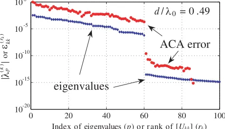
0 20 40 60 80 100

10 -20 10 -15 10 -10 10 -5 100

Index of eigenvalues (p) o r r ank of [Ukk] (rk)

| ( k ) p |o r ( rk )

kk _{ACA error}

eigenvalues

d / λ0 = 0 .49

λ

ε

Figure 5. Low-rank nature of [Skk] for the bricks

used to model the antenna system in Fig. 1: () eigenvalues of [Skk] versus their index; (•) relative

error of the ACA decomposition of [Skk] versus the

rank of [Ukk].

required to generate varying numbers of columns of [Ukk]. Since the time values are quite small anyway, it may well be the case that some unaccounted overhead dominates the calculation rather than the ACA itself. Regardless, it is worthwhile mentioning that the spectral decomposition of the relevant algebraic scattering operator (with size 1320×1320) takes about 33 s, a time which is two orders of magnitude larger than the values of Fig. 4.

Finally, in Fig. 5 we have compared the spectrum of eigenvalues of [Skk] and the ACA error in Eq. (9) at d/λ0 = 0.49. The eigenvalues () are ordered with decreasing magnitude and plotted versus their index p, though only the first 100 eigenvalues are shown. The ACA error (•) is plotted as a function of the rank rk of [Ukk] at each step of the algorithm [29]; in particular, the ACA continues

until the error is smaller than t= 10−15_{. Both the spectrum andε}(rk)

kk exhibit a jump for p=rk = 60,

5. CONCLUSION

We have proposed a methodology based on the ACA algorithm to extract macro basis functions from the low-rank scattering operators [Skk] of LEGO. While the ACA macro basis functions exhibit convergence

properties similar to those of the eigencurrents of [Skk], the former can be generated more quickly than

the latter. The ACA macro basis functions are efficacious at compressing the LEGO algebraic equations for scattering and radiation problems, and have been shown to yield the same results as the eigencurrents.

ACKNOWLEDGMENT

The Author wishes to thank Dr. Rob Maaskant (Chalmers University of Technology, Goteburg, Sweden) for the fruitful discussions on the usage of ACA for the calculation of basis functions and EM fields. The appreciation and the useful remarks from the Reviewers are also gratefully acknowledged.

REFERENCES

1. Peterson, A. F., S. L. Ray, and R. Mittra, Computational Methods for Electromagnetics, IEEE Press, Piscataway, 1998.

2. Harrington, R. F., Field Computation by Moment Methods, MacMillan, New York, 1968.

3. Zienkiewicz, O. C., The Finite Element Method in Engineering Science, McGraw-Hill, London, 1971.

4. Adams, R. J., “Physical and analytical properties of a stabilized electric field integral equation,”

IEEE Trans. Antennas Propag., Vol. 52, 362–372, Feb. 2004.

5. Andriulli, F., K. Cools, H. Bagci, F. Olyslager, A. Buffa, S. Christiansen, and E. Michielssen, “A multiplicative Calderon preconditioner for the electric field integral equation,” IEEE Trans. Antennas Propag., Vol. 56, 2398–2412, Aug. 2008.

6. Stephanson, M. B. and J.-F. Lee, “Preconditioned electric field integral equation using Calderon identities and dual loop/star basis functions,”IEEE Trans. Antennas Propag., Vol. 57, 1274–1279, Apr. 2009.

7. Engheta, N., W. D. Murphy, V. Rokhlin, and M. S. Vassiliou, “The fast multipole method (FMM) for electromagnetic problems,”IEEE Trans. Antennas Propag., Vol. 40, 634–641, Jun. 1992. 8. Hackbusch, W., “A sparse matrix arithmetic based on H-matrices. Part I: Introduction to H

-matrices,”Computing, Vol. 62, No. 2, 89–108, 1999.

9. Kron, G., “A set of principles to interconnect the solutions of physical systems,”Journal of Applied Physics, Vol. 24, No. 8, 965–980, 1953.

10. Li, M.-K. and W. C. Chew, “Wave-field interaction with complex structures using equivalence principle algorithm,” IEEE Trans. Antennas Propag., Vol. 55, 130–138, Jan. 2007.

11. Shao, H., J. Hu, W. Lu, H. Guo, and Z. Nie, “Analyzing large-scale arrays using tangential equivalence principle algorithm with characteristic basis functions,” Proceedings of the IEEE, Vol. 101, 414–422, Feb. 2013.

12. Maaskant, R., R. Mittra, and A. Tijhuis, “Fast analysis of large antenna arrays using the characteristic basis function method and the adaptive cross approximation algorithm,”IEEE Trans. Antennas Propag., Vol. 56, 3440–3451, Nov. 2008.

13. Xiao, G., J.-F. Mao, and B. Yuan, “A generalized surface integral equation formulation for analysis of complex electromagnetic systems,”IEEE Trans. Antennas Propag., Vol. 57, 701–710, Mar. 2009. 14. Yl¨a-Oijala, P. and M. Taskinen, “Electromagnetic scattering by large and complex structures with surface equivalence principle algorithm,”Waves in Random and Complex Media, Vol. 19, 105–125, Feb. 2009.

15. Ol´can, D. I., I. M. Stevanovi´c, J. R. Mosig, and A. R. Djordjevi´c, “Diakoptic approach to analysis of multiconductor transmission lines,” Microwave and Optical Technology Letters, Vol. 50, No. 4, 931–936, 2008.

the subdomain multilevel approach,” Microwave and Optical Technology Letters, Vol. 42, No. 2, 138–143, 2004.

17. Craeye, C., J. Laviada, R. Maaskant, and R. Mittra, “Macro basis function framework for solving Maxwell’s equations in surface-integral-equation form,”Forum for Electromagnetic Research Methods and Application Technologies (FERMAT), Vol. 3, 1–16, May 2014, Online at www.e-fermat.org.

18. Lucente, E., A. Monorchio, and R. Mittra, “An iteration-free MoM approach based on excitation independent characteristic basis functions for solving large multiscale electromagnetic scattering problems,” IEEE Trans. Antennas Propag., Vol. 56, 999–1007, Apr. 2008.

19. Zhang, B., G. Xiao, J. Mao, and Y. Wang, “Analyzing large-scale non-periodic arrays with synthetic basis functions,”IEEE Trans. Antennas Propag., Vol. 58, 3576–3584, Nov. 2010.

20. Lancellotti, V., B. P. de Hon, and A. G. Tijhuis, “An eigencurrent approach to the analysis of electrically large 3-D structures using linear embedding via Green’s operators,” IEEE Trans. Antennas Propag., Vol. 57, 3575–3585, Nov. 2009.

21. Van de Water, A. M., “LEGO: Linear Embedding via Green’s Operators,” Ph.D. thesis, Technische Universiteit Eindhoven, 2007.

22. Lancellotti, V., B. P. de Hon, and A. G. Tijhuis, “Scattering from large 3-D piecewise homogeneous bodies through linear embedding via Green’s operators and Arnoldi basis functions,” Progress In Electromagnetics Research, Vol. 103, 305–322, Apr. 2010.

23. Lancellotti, V. and A. G. Tijhuis, “Extended linear embedding via Green’s operators for analyzing wave scattering from anisotropic bodies,” International Journal of Antennas and Propagation, 11 pages, Article ID 467931, 2014.

24. Lancellotti, V. and D. Melazzi, “Hybrid LEGO-EFIE method applied to antenna problems comprised of anisotropic media,” Forum in Electromagnetic Research Methods and Application Technologies (FERMAT), Vol. 6, 1–19, 2014, Online at www.e-fermat.org.

25. Lancellotti, V., B. P. de Hon, and A. G. Tijhuis, “On the convergence of the eigencurrent expansion method applied to linear embedding via Green’s operators (LEGO),” IEEE Trans. Antennas Propag., Vol. 58, 3231–3238, Oct. 2010.

26. Bebendorf, M., “Approximation of boundary element matrices,”Numer. Matematik, Vol. 86, No. 4, 565–589, 2000.

27. Lancellotti, V. and R. Maaskant, “A comparison of two types of macro basis functions defined on LEGO electromagnetic bricks,” 9th European Conference on Antennas and Propagation (EuCAP 2015), Lisbon, Portugal, Apr. 2015.

28. Lancellotti, V., “Fast generation of macro basis functions for LEGO through the adaptive cross approximation,” International Conference on Electromagnetics in Advanced Applications (ICEAA 2015), Turin, Italy, Sept. 2015, invited paper.

29. Zhao, K., M. Vouvakis, and J.-F. Lee, “The adaptive cross approximation algorithm for accelerated method of moments computations of EMC problems,”IEEE Trans. Electromag. Compat., Vol. 47, 763–773, Nov. 2005.

30. Maaskant, R., R. Mittra, and A. G. Tijhuis, “Fast analysis of large antenna arrays using the characteristic basis function method and the adaptive cross approximation algorithm,”IEEE Trans. Antennas Propag., Vol. 56, 3440–3451, Nov. 2008.

31. Maaskant, R. and V. Lancellotti, “Field computations through the ACA algorithm,” 9th European Conference on Antennas and Propagation (EuCAP 2015), Lisbon, Portugal, Apr. 2015.

32. Collin, R. E.,Field Theory of Guided Waves, IEEE Press, Piscataway, 1991.

33. Press, W. H., S. A. Teukolsky, W. T. Vetterling, and B. P. Flannery,Numerical Recipes in Fortran, 2nd Edition, Cambridge University Press, Cambridge, 1994.