Profile Reconstruction Utilizing Forward-Backward Time-Stepping
with the Integration of Automated Edge-Preserving Regularization
Technique for Object Detection Applications
Guang Yong1, Kismet Anak Hong Ping1, *, Shafrida Sahrani1, Mohamad Hamiruce Marhaban2, Mohd Iqbal Saripan2,
Toshifumi Moriyama3, and Takashi Takenaka3
Abstract—A regularization is integrated with Forward-Backward Time-Stepping (FBTS) method which is formulated in time-domain utilizing Finite-Difference Time-Domain (FDTD) method to solve the nonlinear and ill-posed problem arisen in the microwave inverse scattering problem. FBTS method based on a Polak-Ribi`ete-Polyak conjugate gradient method is easily trapped in the local minima. Thus, we extend our work with the integration of edge-preserving regularization technique due to its ability to smooth and preserve the edges containing important information for reconstructing the dielectric profiles of the targeted object. In this paper, we propose a deterministic relaxation with Mean Square Error algorithm known as DrMSE in FBTS and integrate it with the automated edge-preserving regularization technique. Numerical simulations are carried out and prove that the reconstructed results are more accurate by calculating the edge-preserving parameter automatically.
1. INTRODUCTION
Inverse scattering in microwave imaging has been widely studied by many researchers for last decades. Microwave imaging [1] is a very promising approach for many practical applications. It has huge potential in measuring the characteristic of the embedded objects inside a bounded space region by illuminating electromagnetic waves. Microwave imaging has the ability to retrieve information about the distribution of the dielectric properties space region, the shape and the location of the embedded object. Besides that, microwave imaging has lower cost than other well-known screening approaches, for example, positron emission tomography and computed tomography. Furthermore, microwave imaging is safer with low nonionizing radiation than X-ray mammography. Thus, it is recommended that microwave imaging is applied as a diagnostic tool for several areas which involve civil and industrial engineering [2– 5], nondestructive testing and evaluation [6–10], geophysical prospecting [11] buried object detection for military [12–14] medical diagnostic for biomedical engineering [15–19], and screening tool for wood industry [20].
Solving an inverse scattering problem is a very challenging task due to nonlinearity of the scattering equations, ill-posedness of the problem and uniqueness of the solution [21]. This problem could be dealt with either in frequency-domain or time-domain. The frequency-domain based technique has successfully reconstructed satisfactory results [22, 23], but it showed some drawbacks. Firstly, the use of higher frequencies may improve the spatial resolution, but it leads to highly nonlinear formulation and more complexity when measuring the scattered field. Secondly, collected information is limited
Received 10 November 2016, Accepted 21 January 2017, Scheduled 17 February 2017
* Corresponding author: Kismet Anak Hong Ping ([email protected]).
when using single-frequency data. To overcome this problem, it is suggested to use time-domain based technique. Time-domain based technique has demonstrated the ability to reconstruct the distribution of dielectric properties more accurately [24–28]. Currently, time-domain based technique includes Lagrange multipliers technique by Rekanos [24], time-domain inverse scattering by Winters et al. [25] and FBTS method by Takenaka et al. [26–28].
Since the microwave imaging is a nonlinear inverse scattering problem, the adoption of regularization technique is needed to obtain a stable solution by avoiding the ill-posed nature [29, 30]. The most popular technique is using Tikhonov regularization technique to solve the ill-posed nature [31– 34]. It has been applied in many different fields, and unfortunately, Tikhonov regularization strongly penalizes the discontinuities and smooths the object edges resulting blurred images. This weakness may lead to false result to the observer; for example, a doctor hardly identifies an organ or a tumor correctly due over-smoothed dielectric properties. To overcome this problem, edge-preserving regularization [26, 35] is suggested because it uses local smoothness constraints with account of intensity discontinuities.
In our previous study [36], preliminary results showed that the integration of edge-preserving regularization provided more accurate reconstructed profile. In this paper, we use bigger size and more complicated target object to prove efficiency of the Edge-preserving regularization technique. This technique is extended with automated procedures which has the ability of finding the regularization technique parameters such as weighting parameters and threshold parameters to detect the edges for each iteration. Common regularization technique parameters are exploited by numerical experiment. Based on our experiences, it is not an easy task to find those parameters for the regularization technique. This paper is organized as follows. Section 1 introduces some challenges and problem solving of the microwave imaging approaches. Section 2 explains our proposed method, FBTS integrated with automated Edge-preserving regularization technique. Section 3 presents the numerical results and discussion. Finally, Section 4 concludes the paper.
2. METHOD
2.1. Forward-Backward Time-Stepping Method
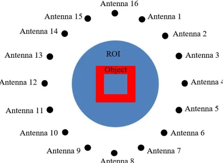
Let us consider a region of interest (ROI) representing the 2D object embedded in a homogeneous medium. The object is assumed inhomogeneous and has different dielectric properties compared to ROI. We assume that the ROI is located in free-space medium and surrounded by 16 antennas as shown in Figure 1. Each antenna will take turn to act as a transmitter, mto transmit Gaussian pulse to ROI and the remaining antennas becoming receiver,nto receive the scattered signals until a combination of 240 transmitter/receiver data set is obtained.
The inverse scattering problem considered here is to reconstruct the dielectric profiles of the ROI
by using the scattered signal collected by the receiver. In Forward-Backward Time-Stepping (FBTS) method, the collected data are formulated as an optimization problem with the form of cost functional Qrec(p) to be minimized as follows:
Qrec(p) =
cT 0 M m=1 N n=1
Wmn(t)|em(p;rn, t)−e˜m(rn, t)|2d(ct) (1)
wherep is a medium parameter vector function given by
p= [p1(r), p2(r)] = [εr(r), σ(r)] r = [x, y, z] (2) In Eq. (1),Wmn(t) is a nonnegative weighting function which takes a value of zero at timet=T(Tis the time duration of the measurement), andem(p;rn, t) and ˜em(rn, t) are the calculated electromagnetic fields in time domain for an estimated medium parameter vector p and the measured electromagnetic fields due to themth source, respectively.
To find the solution of medium parameter p, a gradient-based optimization method is applied to cost functional in Eq. (1). By taking the Fr´echet derivative of Eq. (1), the gradients of medium parameter vector equations are derived as
gεr(r) = cT
0 M
m=1
2um(p;r, t) d
dctem(p;r, t)d(ct) (3)
gσ(r) =
cT
0 M
m=1
2um(p;r, t)em(p;r, t) d(ct) (4)
where um(p;r, t) andem(p;r, t) are the adjoint fields and electromagnetic fields calculated in the ROI, respectively. The adjoint fields,um(p;r, t), are time reversed fields with equivalent current sources which are identical to a difference between the measured and calculated electromagnetic field data. In this paper, Polak-Ribi`ete-Polyak conjugate gradient method is used as optimization technique to solve the inverse scattering problem.
2.2. Edge-Preserving Regularization Technique
Since the inverse scattering problem is nonlinear and ill-posed in the sense of Hadamard [37], an edge-preserving regularization technique is needed to handle this problem. Therefore, the cost functional in Eq. (1) is modified into a new total cost functional equation.
Qtotal (p) =Qrec(p) +Qedge(p) (5)
where the first term, Qrec(p), is residual term as in Eq. (1), and the second term, Qedge(p), is the edge-preserving regularizing term as follows:
Qedge(p) =λεr
S ϕ
∇pεr
χεr
dS+λσ
S ϕ
∇pσ
χσ
dS (6)
In this paper, Sobel operator is used to find the norm of gradient, ∇p
∇p =
p2
x+p2y (7)
px = 1 8
−1 −2 −1
0 0 0
1 2 1
, py = 1 8
−1 0 1
−2 0 2
−1 0 1
preserving regularization term is applied separately on the relative permittivity εr and conductivity σ profile. The weighting parameters λεr and λσ are used to balance the effect of the residual term and regularization term. The threshold parameters χεr and χσ are used to determine the value of the gradient norm of which discontinuity is preserved without smoothing it. Note that many researchers have used numerical observation to determine the parameters ofλand χ [26, 41].
In this work, we develop two automated procedures with a simple calculation to automatically determine the regularization technique parameters for each iteration. Firstly, the weighting parameters λare calculated based on the gradient values of Eqs. (3) and (4), respectively. Secondly, the values of the threshold parameters χ are calculated based on half of the highest value of the norm of gradient ∇p in the ROI.
Suppose that Qedge(p) has a minimum in p, but to find the minimum, it is a difficult task due to nonlinearity [35]. Thus, in order to make the minimization simple, the potential function can be modified as in [42].
ϕGM(t) = bt2+ψ(b)
(8)
where the expression of ψ(b) is b−2√b+ 1, and b is auxiliary vector also known as the discontinuity reference.
bGM =
1
1 + (∇p/χ)2 (9)
Then, the regularization term Qedge(p) can be modified into half-quadratic regularization term, Qedge(p, b)
Qedge(p, b) =λεr
S
bεr
∇pεr2
χ2 εr
+ψ(bεr)
dS+λσ
S
bσ∇ pσ2 χ2
σ
+ψ(bσ)
dS (10)
Hence, the total cost functional will be evolved as
Qtotal(p, b) =Qrec(p) +Qedge(p, b) (11) By taking the Fr´echet derivative of Eq. (10), the gradients of medium parameter vector for the new edge-preserving regularization term are derived as
gi(r) =−2 λi
χ2i∇ ·(bi∇pi), i=εr, σ (12)
Thus, the total gradient is obtained as
gtotal(r) =gF BT S,i(r) +gEdge,i(r), i=εrσ (13)
2.3. Deterministic Relaxation with Mean Square Error (DrMSE) Algorithm
In order to solve the total cost functional that expressed as in Eq. (11), we introduce alternate minimizations scheme over p and b. When the auxiliary vector b is fixed, the edge-preserving regularization term Qedge(p, b) is quadratic in p. Thus, the minimization of Eq. (11) can be performed by the Polak-Ribi`ete-Polyak conjugate gradient method. Whenpis fixed, the values ofbare analytically obtained for each point (x, y) in each profile with Eq. (9). In order to control this scheme, we propose the integration of Mean Square Error (MSE) with the deterministic relaxation processes.
M SE= 1
XY X x=1 Y y=1
pn+1(x, y)−pn(x, y)2 (14)
wherepn+1 is the current dielectric profile,pn the previous dielectric profile, and X,Y are the point of the profile.
Begin, setn= 0
Reconstruct initial profile p0
Reconstruct initial auxiliary vector b=b0 Repeat
Reconstruct new profile pn+1 by minimize Qtotal(pn, b) Compute MSE by usingpn+1 andpn
if MSE<1e-6
Reconstruct new auxiliary vector b=bn+1 Endif
Until convergence.
3. RESULTS AND DISCUSSION
In this work, we consider an object embedded in the ROI as an unknown scatterer and surrounded by 16 antennas as shown in Figure 1. In FBTS reconstruction algorithm, we use 1 mm×1 mm cell size for the FDTD lattice. The antennas will take turn to transmit sinusoidally modulated Gaussian pulse with center frequency, fc of 2 GHz with bandwidth of 1.3 GHz. Convolutional Perfectly Matched Layer
(a) (b)
(c) (d)
Dotted area
(CPML) with thickness of 15 mm as an absorber is added at the borders of the FDTD lattice. This CPML has the ability to prevent the reflections of the signal at the boundary of the FDTD lattice and helps to save computation time during numerical simulation work.
In the setup, a 50 mm radius circular shape ROI with the relative permittivity εr = 9.98 and conductivity σr= 0.18 S/m is immersed in a free-space medium. A 20 mm×20 mm rectangular shape with a 8 mm×8 mm void rectangular shape of object is embedded at the center of ROI. This object has the relative permittivity of 21.45 and conductivity of 0.45 S/m. Assume that apriori known profile with the relative permittivity of 13.7 and the conductivity of 0.18 S/m which is slightly near the original profile of ROI as initial guess p0.
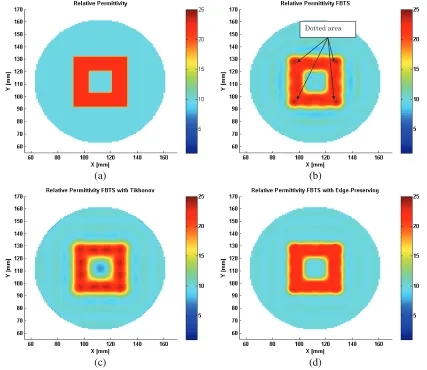
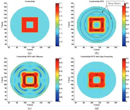
In this work, all numerical simulations are carried out up to 200 iterations. The original profile, FBTS reconstructed profile, FBTS with Tikhonov regularization technique reconstructed profile and FBTS with automated Edge-preserving regularization technique reconstructed profile images for the object relative permittivity spatial distribution are illustrated in Figure 2. Figure 3 shows the corresponding conductivity spatial distribution. As shown in Figure 2 and Figure 3, all these techniques have successfully reconstructed the location and shape of the embedded object in ROI. However, there are enormous different reconstructed profile images for these three techniques.
In FBTS method, the reconstructed profile successfully points out the location and shape of the embedded object. However, for the reconstructed relative permittivity profile, some dotted areas at
(a) (b)
(c) (d)
Ring Object
the edges of the object can be observed as illustrated in Figure 2(b). As for the reconstruction of conductivity, the reconstructed image having a rough surface within the ROI. Two unknown ring objects are marked in dotted circle as illustrated in Figure 3(b). These reconstructed profile images give false reading where it may indicate that some other objects exist in the ROI. We believe that the results are trapped in local minima during the optimization process.
In order to avoid being trapped in local minima, regularization is needed. In this paper, the profile of reconstruction for two different regularization techniques is presented. The first one is the Tikhonov regularization technique, and the second is the proposed automated edge-preserving regularization technique. In FBTS with Tikhonov regularization technique, the reconstructed relative permittivity profile is improved as shown in Figure 2(c). However, for the reconstructed conductivity profile, the shape of the embedded object is changed from rectangle to circle, and the ring object in ROI can be clearly identified as shown in Figure 3(c). This occurs due to over-smoothing by the Tikhonov parameters.
In order to solve the over-smoothing effect, automated edge-preserving regularization technique is then proposed to preserve the edge while smoothing. As shown in Figure 2(d) and Figure 3(d), the FBTS with automated Edge-preserving regularization technique reconstructs more accurate profile than the other two techniques. In the result, no dotted area appears as shown in Figure 2(b), and there is no ring object presented in the ROI. It is believed that those false results are smoothed while maintaining the shape of embedded object. Thus, the FBTS with automated edge-preserving regularization technique provides a solution in smoothing the dotted area and ring object while preserving the edge of the embedded object.
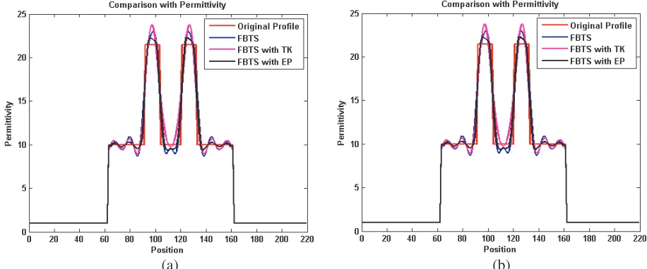
In Figure 4, the cross-sectional views at axis x = 107 for relative permittivity and conductivity profiles are presented. It shows that the edges are smoothed when FBTS method is applied with the integration of Tikhonov regularization technique. However, the reconstructed results show that the ROI and embedded object are improved while the edges are preserved when FBTS integrated with automated edge-preserving regularization technique is applied.
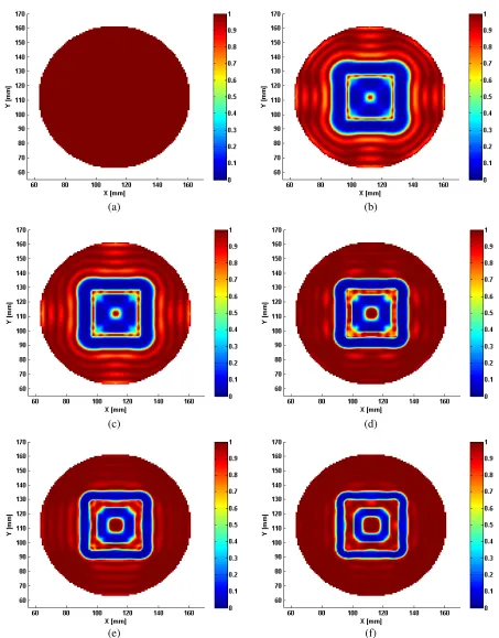
The computed auxiliary variables for relative permittivity profile during simulation are obtained as illustrated in Figure 5. The initial step for the auxiliary variables is initialized as shown in Figure 5(a). The initial auxiliary variables at first iteration are assumed homogeneous and uniformly equal to 1. The weighting parametersλare calculated automatically to the nearest decimal value of gradient as in Eq. (3). This will automatically stabilized both terms in Eq. (13).
At Step 1, new auxiliary variables are computed when the MSE for the current profile pn+1 and previous profile pn is less than 1e-6 as shown in Figure 5(b). The threshold values χ are calculated to determine the discontinuity or edge in the reconstructed profile. It is based on half of the highest value
(a) (b)
(a) (b)
(c) (d)
(e) (f)
of the norm of gradient ∇p. If the values are higher than χ, it is assumed as edge and needs to be preserved. This discontinuity or edge maps are roughly estimated and introduced for following profile estimate, and so on.
As the DrMSE algorithm proceeds, the auxiliary variables will become more precise as shown in Figure 5. At each step, new auxiliary variables are introduced, and the profile reconstruction becomes closer to actual profile. The DrMSE procedure takes 51 steps to reconstruct the relative permittivity profiles. Figure 5(b) through Figure 5(f) give the auxiliary variables for steps 1, 5, 15, 30 and 51 which take part in the 50th, 70th, 103th, 133th, and 188th iterations, respectively. Meanwhile, DrMSE procedure takes 45 steps to reconstruct the conductivity profile.
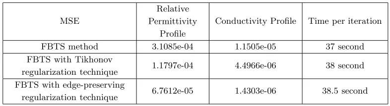
Figure 2 through Figure 4, FBTS integrated with automated Edge-preserving regularization technique yields better accurate result than FBTS method only and FTBS integrated with Tikhonov regularization technique. It is also proven by using MSE comparison of reconstructed dielectric profile and original profile as shown in Table 1. It shows that FBTS with edge-preserving regularization technique gives the smaller error than the other two techniques. All three numerical simulations only take about 40 seconds per iteration.
Table 1. MSE comparison and time per iteration.
MSE
Relative Permittivity
Profile
Conductivity Profile Time per iteration
FBTS method 3.1085e-04 1.1505e-05 37 second FBTS with Tikhonov
regularization technique 1.1797e-04 4.4966e-06 38 second FBTS with edge-preserving
regularization technique 6.7612e-05 1.4303e-06 38.5 second
4. CONCLUSIONS
Since the inverse scattering problem has nonlinear and ill-posed nature, edge-preserving regularization is integrated with FBTS method to avoid being trapped in the local minima during the minimization of cost functional. In this paper, we use DrMSE algorithm to control the alternate minimization scheme. Besides, the weighting parametersλand threshold parametersχare automatically decided by automated procedures iteratively. From the results, the FBTS with automated edge-preserving regularization technique has been successfully reconstructed with more accurate relative permittivity and conductivity profiles than using FBTS method only and FBTS with Tikhonov regularization technique. Therefore, we will extend this research to focus on more complicated and/or realistic model for our future research works.
ACKNOWLEDGMENT
This research was supported by Research Acculturation Collaborative Effort (RACE) grant scheme (RACE/c(3)/1332/2016(5)).
REFERENCES
1. Pastorino, M., Microwave Imaging, 1st edition, John Wiley, Hoboken, N.J., 2010.
2. Kim, Y. J., L. Jofre, F. De Flaviis, and M. Q. Feng, “Microwave reflection tomographic array for damage detection of civil structures,”IEEE Trans. Antennas Propag., Vol. 51, No. 11, 3022–3032, 2003.
monitoring and biological bodies inspection,” IEEE Trans. Instrum. Meas., Vol. 55, 1878–1884, 2006.
4. Langenberg, K. J., K. Mayer, and R. Marklein, “Nondestructive testing of concrete with electromagnetic and elastic waves: Modeling and imaging,” Cem. Concr. Compos., Vol. 28, No. 4, 370–383, 2006.
5. Randazzo, A. and C. Estatico, “A regularisation scheme for electromagnetic inverse problems: Application to crack detection in civil structures,” Nondestruct. Test. Eval., Vol. 27, No. 3, 189– 197, 2012.
6. Qaddoumi, N., R. Zoughi, and G. W. Carriveau, “Microwave detection and depth determination of disbonds in low-permittivity and low-loss thick sandwich composites,”Res. Nondestruct. Eval., Vol. 8, No. 1, 51–63, 1996.
7. Kharkovsky, S. and R. Zoughi, “Microwave and millimeter wave nondestructive testing and evaluation — Overview and recent advances,” IEEE Instrum. Meas. Mag., Vol. 10, No. 2, 26– 38, 2007.
8. Zoughi, R. and S. Kharkovsky, “Microwave and millimetre wave sensors for crack detection,”Fatigue Fract. Eng. Mater. Struct., Vol. 31, No. 8, 695–713, 2008.
9. Deng, Y. and X. Liu, “Electromagnetic imaging methods for nondestructive evaluation applications,” Sensors, Vol. 11, No. 12, 11774–11808, 2011.
10. Zoughi, R., Microwave Non-destructive Testing and Evaluation, Kluwer, The Netherlands, 2000. 11. Pastorino, M., “Recent inversion procedures for microwave imaging in biomedical, subsurface
detection and nondestructive evaluation applications,” Measurement: Journal of the International Measurement Confederation, Vol. 36, No. 3–4, 257–269, 2004.
12. Pastorino, M. and A. Randazzo, “Buried object detection by an inexact newton method applied to nonlinear inverse scattering,”Int. J. Microw. Sci. Technol., Vol. 2012, 2012.
13. Estatico, C., A. Fedeli, M. Pastorino, and A. Randazzo, “Buried object detection by means of a L p Banach-space inversion procedure,”Radio Sci., Vol. 50, No. 1, 41–51, Jan. 2015.
14. Rufus, E. and Z. C. Alex, “Microwave imaging system for the detection of buried objects using UWB antenna — An experimental study,”PIERS Proceedings, 786–788, Kuala Lumpur, Malaysia, Mar. 27–30, 2012.
15. Hagness, S. C., “Microwave imaging in medicine: Promises and future challenges,” Proc. URSI Gen. Assem., 53706, 2008.
16. Semenov, S., “Microwave tomography: Review of the progress towards clinical applications,” Philos. Trans. A. Math. Phys. Eng. Sci., Vol. 367, 3021–3042, 2009.
17. Meaney, P. M., K. D. Paulsen, and D. College, “Challenges on microwave imaging supported by clinical results,”Proc. Int. Work. Biol. Eff. Electromagn. Fields, 10–14, 2010.
18. Hassan, M. and A. M. El-Shenawee, “Review of electromagnetic techniques for breast cancer detection,”IEEE Rev. Biomed. Eng., Vol. 4, 103–118, 2011.
19. Wei, N. S., K. A. H. Ping, L. S. Yee, W. A. B. W. Zainal Abidin, T. Moriyama, and T. Takenaka, “Reconstruction of extremely dense breast composition utilizing inverse scattering technique integrated with frequency-hopping approach,” ARPN J. Eng. Appl. Sci., Vol. 10, No. 18, 8479– 8484, 2015.
20. Salvad, A., M. Pastorino, R. Monleone, A. Randazzo, T. Bartesaghi, G. Bozza, and S. Poretti, “Microwave imaging of foreign bodies inside wood trunks,” IST 2008 — IEEE Workshop on Imaging Systems and Techniques Proceedings, 88–93, 2008.
21. Colton, D. and R. Kress,Inverse Acoustic and Electromagnetic Scattering Theory, Springer, New York, 2012.
22. Massa, A., D. Franceschini, G. Franceschini, M. Pastorino, M. Raffetto, and M. Donelli, “Parallel GA-based approach for microwave imaging applications,”IEEE Trans. Antennas Propag., Vol. 53, No. 10, 3118–3127, 2005.
Vol. 53, No. 5, 1761–1776, 2005.
24. Rekanos, I. T., “Time-domain inverse scattering using Lagrange multipliers: An iterative FDTD-based optimization technique,”Journal of Electromagnetic Waves and Applications, Vol. 17, No. 2, 271–289, 2003.
25. Winters, D. W., E. J. Bond, B. D. Van Veen, and S. C. Hagness, “Estimation of the frequency-dependent average dielectric properties of breast tissue using a time-domain inverse scattering technique,”IEEE Trans. Antennas Propagat., Vol. 54, No. 11, 3517–3528, 2006.
26. Takenaka, T., H. Jia, and T. Tanaka, “Microwave imaging of electrical property distributions by a forward-backward time-stepping method,” Journal of Electromagnetic Waves and Applications, Vol. 14, No. 12, 1609–1626, 2000.
27. Takenaka, T., T. Tanaka, H. Harada, and S. He, “FDTD approach to time-domain inverse scattering problem for stratified lossy media,”Microw. Opt. Technol. Lett., Vol. 16, No. 5, 292–296, 1997. 28. Ping, K. A. H., T. Moriyama, T. Takenaka, and T. Tanaka, “Two-dimensional forward-backward
time-Stepping approach for tumor detection in dispersive breast tissues,” 2009 Mediterranean Microw. Symp. (MMS), 1–4, 2009.
29. Blanc-Feraud, L., P. Charbonnier, G. Aubert, and M. Barlaud, “Nonlinear image processing: Modeling and fast algorithm for regularization with edge detection,” Proc. IEEE-ICIP, 474–477, 1995.
30. Lobel, P., C. Picbota, L. Blanc Feraud, and M. Barlaud, “Conjugate gradient algorithm with edge-preserving regularization for image reconstruction from experimental data,” IEEE Antennas Propag. Soc. Int. Symp. 1996, AP-S. Dig., Vol. 1, 644–647, 1996.
31. Chew Chie, A. S., K. A. Hong Ping, Y. Guang, N. S. Wei, and N. Rajaee, “Preliminary results of integrating Tikhonov’s regularization in Forward-Backward Time-Stepping technique for object detection,”Appl. Mech. Mater., Vol. 833, 170–175, Apr. 2016.
32. Kaltenbacher, B., A. Kirchner, and B. Vexler, “Adaptive discretizations for the choice of a Tikhonov regularization parameter in nonlinear inverse problems,” Inverse Probl., Vol. 27, No. 12, 125008, Dec. 2011.
33. Qin, Y. M. and I. R. Ciric, “Dielectric body reconstruction with current modelling and Tikhonov regularisation,” Electron. Lett., Vol. 29, No. 16, 1427, 1993.
34. Calvetti, D., S. Morigi, L. Reichel, and F. Sgallari, “Tikhonov regularization and the L-curve for large discrete ill-posed problems,”J. Comput. Appl. Math., Vol. 123, 423–446, 2000.
35. Charbonnier, P., L. Blanc-F´eraud, G. Aubert, and M. Barlaud, “Deterministic edge-preserving regularization in computed imaging,” IEEE Trans. Image Process., Vol. 6, No. 2, 298–311, 1997. 36. Yong, G., K. A. H. Ping, A. S. C. Chie, S. W. Ng, and T. Masri, “Preliminary study
of Forward-Backward Time-Stepping technique with edge-preserving regularization for object detection applications,” 2015 International Conference on BioSignal Analysis, Processing and Systems (ICBAPS), 77–81, 2015.
37. Hadamard, J., “Lectures on Cauchy’s problem in linear partial differential equations,”Physiology, 334, 1923.
38. Hebert, T. and R. Leahy, “A generalized EM algorithm for 3-D Bayesian reconstruction from Poisson data using Gibbs priors,”IEEE Trans. Med. Imaging, 194–202, 1989.
39. Green, P. J., “Bayesian reconstructions from emission tomography data using a modified EM algorithm,”IEEE Trans. Med. Imaging, Vol. 9, No. 1, 84–93, Mar. 1990.
40. Geman, S. and D. E. M. Clure, “Bayesian image analysis: An application to single photon emission tomography,”Proc. Stat. Comput. Sect., 12–18, 1985.
41. Aubert, G., M. Barlaud, L. Blanc-Feraud, and P. Charbonnier, “A deterministic algorithm for edge-preserving computed imaging using Legendre transform,” Proceedings of the 12th IAPR International Conference on Pattern Recognition (Cat. No. 94CH3440-5), 188–191, 1994.