Polarimetric Target Detection Using Statistic of the Degree
of Polarization
Bo Ren1, 2, *, Longfei Shi1, 2, and Guoyu Wang1, 2
Abstract—The degree of polarization (DoP) can be utilized as a detection statistic in the polarimetric radar to achieve target detection performance improvement. In this paper, a polarimetric radar model is established, which includes reflections from both target and clutter at first. Then, probability density functions (PDFs) of the estimated DoP are expressed in closed form, which is derived from joint eigenvalue distributions of complex noncentral Wishart matrices. The detector is developed and evaluated theoretically on the basis of the statistical properties of the DoP. Finally, a comparison between the new DoP detector and single-polarization detector is presented against real data. The performance improvement is demonstrated by the comparison results.
1. INTRODUCTION
In recent years, most radar systems have the ability to transmit and receive electromagnetic waves at orthogonal polarization (i.e., horizontal and vertical). The polarization information has become an important tool for improving target detection performance from the clutter and jammer background [1, 2].
Since the optimum polarization detector has been designed by Novak et al. in 1989 [2], many polarimetric detection algorithms have been subsequently developed [3–5]. Most of these detectors are based on the Kelly’s generalized likelihood ratio (GLR) test [6], which assumes that the clutter covariance can be well estimated by the training data or can be obtained as priori knowledge. This may not be reasonable, especially when the targets exist in nonhomogeneous clutter environment. Moreover, the full polarization scattering matrix (PSM) has to be measured in order to carry on those detectors. However, lots of radar systems can only operate at a dual-polarization mode, at which a single polarization is transmitted, and two orthogonal polarizations (i.e., denoted HH and HV) are received. To overcome the above problems, an important variable available to characterize polarization for polarimetric radar shall be considered as a new detection statistic in this paper, which is the degree of polarization (DoP). In studies of partially polarized planar waves, the DoP is defined as the ratio of the power of the waves’ fully polarized components to its total power and is obtained from Wolf’s polarization covariance matrix (PCM) [7, 8]. It has been demonstrated that the physical meaning of the DoP can always be preserved [9, 10]. Furthermore, as an eigenvalue-derived variable, the DoP is independent of the received polarimetric channels chosen to sample the electromagnetic wave.
In practice, the real DoP must be estimated via finite radar received vector samples, which are normally described as random variables because of the random nature of the partially polarized waves. The applications of the DoP statistical properties have already been widely carried out in radar research, geophysics, and optics [11–14]. Specifically, it is found that the mean of the estimated DoP can provide discriminating information for various terrain types such as urban, vegetation, and ocean during the Pol-SAR data research in [11]. Moreover, the estimated DoP can be used as test statistics to detect
Received 10 December 2015, Accepted 23 February 2016, Scheduled 25 February 2016 * Corresponding author: Bo Ren ([email protected]).
the man-made metallic objects (including high-voltage transmission towers, ships, buoys and so on) in clutter environments or to monitor oil spills on the surface of the ocean [12]. In this paper, we mainly focus on the performance improvement of the DoP detector with respect to the other polarimetric detectors, which has not been evaluated yet.
The statistical properties of the DoP shall be obtained in order to assess the detection performance. Based on bivariate complex Gaussian distributions with zero means, the PDFs of the estimated DoP are derived from the joint distributions of the Stokes vector in [13]. They can also be derived from the joint eigenvalue distributions of the polarization covariance matrix in [14], where the polarization covariance matrix is a complex central Wishart matrix. However, when considering a real target embedded in clutter, the complex Gaussian with zero means will be a rough approximation. Anon-zero-mean complex Gaussian radar model has been established in [5]. Thus, the DoP statistic, which is used for describing echoes including both targets and clutter, can be obtained from this model.
In the following section, a basic polarimetric radar measurement model is introduced, and the echoes for both target and clutter are described by statistical models. With an assumption of a distribution with non-zero means, the polarization covariance matrix of the range cell including targets follows a complex noncentral Wishart distribution. Based on the PDF of joint eigenvalues of the PCM, the statistics of the DoP for the range cells with or without targets are derived in Section 3. Using the DoP as a detection statistic, a new detector is designed in Section 4. The theoretical performance of the proposed detector is analyzed in this section. Then, in Section 5 the application of the DoP detector and some other typical polarimetric detectors against real data are presented. The performance improvement of the new proposed detector can be demonstrated by the comparison results. Concluding components are provided in Section 6.
2. RADAR RETURN MODEL
We consider that a target with deterministic PSM is being illuminated by polarimetric radar, which has the ability of dual-polarization simultaneous reception (i.e., horizontal and vertical reception). The radar returns also include clutter signals surrounding the target echoes. Specially, the clutter in the main beam of the radar is mainly considered in this paper. Thereupon, the radar return corresponding to the range cell that the target exists can be established as the following model:
H1 :x=Shta+c+n (1)
whereH1 denotes the target-present hypothesis,
S=
shh shv
svh svv
is the 2×2 PSM of the target, which represents the polarization change of the transmitted signal; htis the 2×1 polarization Jones vector of the transmitted electromagnetic wave; aincludes the transmitted radar waveform and information of the range and Doppler. The second term in the right side of Equation (1) represents the clutter signals. nis the noise in each polarimetric channel. We assume that the target exists in only one range cell. Then in other range cells, the signal model satisfies target-free hypothesis H0, which is given by
H0 :x=c+n. (2)
In the clutter-only range cell, the radar returns consist of the reflections from large number of random scattering points. Then, the measurement data x in H0 case follows the bivariate complex Gaussian
distribution with zero means
fH0(x) =
1
π2|Σ|exp
−xHΣ−1x, x∈C2 (3)
whereH denotes the Hermitian transpose,Σthe covariance matrix, and|Σ|the determinant ofΣ. On the other hand, when both the target and clutter exist in the range cell under test, x in H1
case is a non-zero-mean complex Gaussian random vector. In this case, the PSM, the relative position and attitude of the target can be considered as constant during pulses in the radar dwell. Then the mean vector ofx is defined as
and covariance matrix is
Σ=E
(x−s) (x−s)H
then its PDF can be obtained from [15] as
fH1(x) =
1
π2|Σ|exp
−(x−s)HΣ−1(x−s) , x∈C2 (4)
Assuming that the radar dwell duration consists ofK pulses, we can obtain Kobservation samples for radar returns in each range cell. The kth observation sample for a range cell is defined as a Jones vector xk = [xH,k xV,k]T. H and V in the subscript denote a set of horizontal and vertical reception polarization basis. Obviously, the random vector xk follows the PDF in (4) or (3) as the target exists or not. It is worthwhile to notice thatfH1(x)→fH0(x) ass→0, when comparing formula (4) and (3).
3. STATISTICS OF THE DOP
It is well known that the target detection problem is to make decision of choosing hypothesis between
H0 and H1. In this section, we introduce the degree of polarization as a novel detection statistic. In
order to design the target detector by using this statistic, the statistical properties of the DoP should be analyzed in different hypothesis test situations.
As we know, the degree of polarization can be used to characterize the polarization state of the partially polarized waves. We can obtain this parameter from the Stokes vector or polarization covariance matrix. The latter is considered in this paper. Then, the DoP pcan be defined in [8] as
p
tr (Σ)2−4|Σ|
tr (Σ) =
η2−η1 η2+η1.
(5)
where tr(Σ) denotes the trace ofΣ,η1 andη2 (η2 ≥η1) are the eigenvalues ofΣ. Since we have no prior
knowledge about the covariance matrix in real application, it should be estimated from the measurement data. According to the definition of the PCM in [7], the estimation of the PCM Σˆ can be generated from a set of observation samplesx1,x2, . . . ,xK as follows:
ˆ
Σ 1
K
K−1
k=0
xkxHk (6)
where K is the integrated number of samples. If the eigenvalues of Σˆ are ˆη1 and ˆη2, then the sample
estimate of the DoP is defined as
ˆ
p ηˆ2−ηˆ1
ˆ
η2+ ˆη1.
(7)
As we discussed at the end of last section, the hypothesisH0 can be considered as a special case of
H1. Sincexk follows the PDF in (4), let Ξ=
K−1
k=0
xkxHk =KΣˆ, then the matrix Ξfollows the complex
noncentral Wishart distribution withK degrees of freedom, whenK ≥2. The PDF ofΞis given in [16] as
fW(Ξ) =e−tr(Θ)0F˜1(K;ΘΣ−1Ξ)fWC(Ξ) (8)
where ΘΣ−1ssH is the non-centrality matrix, and tr(Θ) designates the trace of Θ. 0F˜1(.;.) in Eq.
(8) is the Bessel-type hypergeometric function, a special case of the generic hypergeometric function of matrix argument in the complex field, defined as a series of complex zonal polynomials in [16]. fWC(Ξ) is the complex central Wishart distribution, whose PDF takes the form
fWC(Ξ) = |Ξ| K−2
πΓ(K)Γ(K−1)|Σ|Ke
[−tr(Σ−1Ξ)] (9)
3.1. Joint Eigenvalue Distributions of Polarization Covariance Matrices
Suppose that Λ = diag(λ1, λ2) and M = diag(μ1, μ2) are the eigenvalue matrices of Σ−1Ξ and Θ,
respectively. The entries of the two diagonal matrices λ2 ≥λ1 andμ2 ≥μ1 are real, sinceΣ−1Ξand Θ
are both 2×2 Hermitians. From James’ results in [16], the joint distribution of the ordered eigenvalues (λ1, λ2) corresponding toΣ−1Ξcan be written as
f(λ1, λ2) = e
(−trM)e(−trΛ)
Γ(K)Γ(K−1)0F˜1(K; M,Λ) (λ1λ2) K−2(
λ2−λ1)2 (10)
where0F˜1(·;·,·) is the hypergeometric function of 2 matrix arguments. Utilizing the theorem 4.2 in [17],
the hyper-geometric function in Eq. (10) can be extended as
0F˜1(K; M,Λ) =
Γ(K)(0F1(K−1;λiμj))2
Γ(K−1)(μ2−μ1)(λ2−λ1)
(11)
where |(f(i, j))2| denotes the determinant of a 2×2 matrix, f(i, j) the matrix element in the ith row and jth column, and 0F1(.;.) a special case of the generalized hypergeometric function defined as [18]
pFq(a1, a2, . . . , ap;b1, b2, . . . , bq;z)
∞
τ=0
(a1)τ(a2)τ. . .(ap)τ
(b1)τ(b2)τ. . .(bq)τ zτ
τ! (12)
where (α)n= Γ(α+n)/Γ(α). In terms of the denominator in (11), λ1 =λ2 andμ1=μ2 are required to
ensure the formula meaningfully. However, because of the presence of the term (λ2−λ1)2 in Eq. (10),
the requirement thatλ1 should be different withλ2 can be relaxed. Substituting Eq. (11) into Eq. (10),
the joint distribution of (λ1, λ2) is given by
ffr(λ1, λ2) = e
−(μ1+μ2+λ1+λ2)(λ
1λ2)K−2(λ2−λ1)
Γ(K−1)2(μ
2−μ1) ·
(0F1(K−1;λiμj))2. (13)
In terms of the definition of the non-centrality matrixΘ, it is the product of the inverse of the covariance matrixΣand the outer productssHof the mean vectors. Due to the rank-one termssH, it is worthwhile
to notice that Θhas at most rank one, i.e., it has at least one zero eigenvalue. First, we consider the case that only one eigenvalue of Θ is zero, i.e., μ2 > μ1 = 0, we can call it rank-1 case. According to
lim
z→00F1(a;z) = 1 and taking the limit of (13) as μ1 →0, the joint PDF of (λ1, λ2) can be reduced to
fr1(λ1, λ2) = e
−(λ1+λ2+μ2)(λ
1λ2)K−2(λ2−λ1)
Γ(K−1)2μ
2 ·
[0F1(K−1;λ2μ2)−0F1(K−1;λ1μ2)]. (14)
Second, two eigenvalues of Θ are both zero in the so-called rank-0 case, i.e., μ2 = μ1 = 0. Applying
L’Hospital’s rule in taking the limit of the joint PDF in Eq. (14) and using
∂0F1(n;az)
∂z =
a0F1(n+ 1;az)
n (15)
yields
fr0(λ1, λ2) = lim
μ2→0fr1(λ1, λ2;μ2) =
e−(λ1+λ2)(λ
1λ2)K−2(λ2−λ1)2
Γ(K)Γ(K−1) . (16)
The joint eigenvalue PDFs of Σ−1Ξ have been expressed in closed forms for different cases. It is easy to found that rank-1 and rank-0 cases are just corresponding toH1 andH0hypotheses, respectively.
PDFs of the estimated DoP in each case can be derived through variable transformation and marginal PDF calculation next.
3.2. PDFs of the Estimated Degree of Polarization
covariance matrix can be denoted asΣ=σ2I2, whereI2 is the 2×2 identity matrix andσ2 the clutter power in each polarization basis.
In terms of the definition of Ξand Σ, the maximum likelihood estimator of the true polarization covariance matrix can be denoted asΣˆ =σ2Σ−1Ξ/K. Then the relations between eigenvalues of Σˆ
and Σ−1Ξ can be established as ˆη1 =σ2λ1/K and ˆη2 =σ2λ2/K. Substituting the relations into Eq.
(7), the estimated DoP is given by
ˆ
p= σ2
Kλ2−σ 2
Kλ1
σ2
Kλ2+σ 2
Kλ1
= λ2−λ1
λ2+λ1.
(17)
We consider the rank-1 case at first. Given the joint PDF of (λ1, λ2) in Eq. (14), we can transform
to the new variables ˆp = (λ2−λ1)/(λ2+λ1) and q =λ2−λ1 by the standard formula for the change
of variables in PDFs. For this transformation, the Jacobian can be denoted as
J
λ1, λ2
ˆ
p, q
=q/(2ˆp2). (18)
Then we can find the joint distribution of (ˆp, q)
fr1(ˆp, q) = e
−μ2(1−pˆ2)K−2
22K−3Γ(K−1)2μ
2pˆ2K−2e
−pqˆq2K−2·
0F1
K−1;(1+ ˆp)μ2 2ˆp q
−0F1
K−1;(1−pˆ)μ2 2ˆp q
. (19)
Integration over q from 0 to∞ using the Equation (7.522-9) in [18] yields
fr1(ˆp) =
Γ(2K−1)e−μ2(1−pˆ2)K−2pˆ
22K−3Γ(K−1)2μ
2 ·
1F1
2K−1;K−1;1+ ˆp 2 μ2
−1F1
2K−1;K−1;1−pˆ 2 μ2
(20)
where 1F1(.;.;.) is the confluent hypergeometric function, also a special case of the generalized
hypergeometric series defined inEq. (12).
We define SCR as ratio of the target echoes power to the total power of clutter. According to the definition ofΘand μ1 = 0, we have
μ2 = tr (Θ) = s2
σ2 = 2SCR. (21)
wheres2 is the power of the target echoes, and 2σ2 the total clutter power. From Eqs. (20) and (21), we can easily find that the PDF of ˆp in rank-1 case has relation with not only the number of samples but SCR as well.
In rank-0 case, similar variable transformation from (λ1, λ2) to (ˆp, q) and marginal integration over q can be done to Eq. (10). Then the PDF fr0(ˆp) can be given as
fr0(ˆp) =
Γ(2K)(1−pˆ2)K−2pˆ2
22K−3Γ(K)Γ(K−1). (22)
The result in Eq. (22) is identical to the PDF in [10], as the real DoPP →0. Since the eigenvalues ofΘ
are both zero in rank-0 case, none of the deterministic polarization components exist in radar reception. Consequently, the polarization covariance matrix degrades to the central Wishart distribution, and the real DoP approximates to 0. As can be noted in Eq. (22), the PDF of ˆp in this case is merely the function of the number of samples.
4. DETECTION TEST AND PERFORMANCE
The novel detection statistic is defined as
TDoP = ˆp. (23)
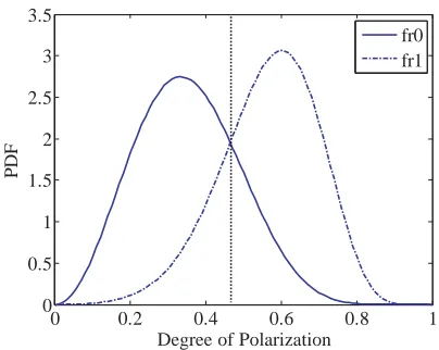
An illustration of the PDFs for the DoP hypothesis test is shown in Fig. 1. Then the detector decides
0 0.2 0.4 0.6 0.8 1 0
0.5 1 1.5 2 2.5 3 3.5
Degree of Polarization
fr0 fr1
Figure 1. PDFs for the DoP hypothesis test.
0 0.2 0.4 0.6 0.8 1
0 0.2 0.4 0.6 0.8 1
Threshold γ
Probability of false alarm
K=8 K=32 K=64
Figure 2. Probability of false alarm of the detector as a function of the threshold, for different sample number K.
lines in Fig. 1. According to the results obtained in last section, the detection statistic is distributed as follows:
TDoP ∼
fr0(ˆp) underH0
fr1(ˆp) underH1 . (24)
Thus, the probability of false alarm can be expressed as follows:
PF A=P(TDoP > γ|H0) =
1
γ fr0(ˆp)dpˆ= 1−
γ
0
fr0(ˆp)dpˆ= 1− Bγ
2(K−1,32)
B(K−1,32) (25)
whereB(a, b) andBα(a, b) are beta function and incomplete beta function, respectively. It is worthwhile to mention that the expression for PF A has only relationship with the thresholdγ and sample number
K. Consequently, the DoP detector is a CFAR test. Fig. 2 shows the probability of false alarm as a function of the threshold γ for sample number K = 8,32 and 64. As can be easily noted that PF A decreases asγ increases. In addition, thePF Acurve becomes steeper as the sample numberK increases. According to the requiredPF A, the thresholdγ can be determined by Eq. (25). Then the detection probability can be obtained by
PD =
1
γ fr1(ˆp)dpˆ=Qfr1(γ) (26) whereQ denotes the right-tail probability function.
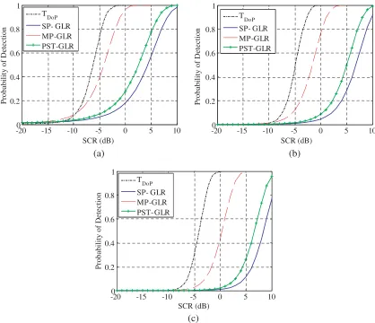
To evaluate the performance improvement, the DoP detector is compared with some other typical polarimetric detectors. The single-polarization generalized likelihood ratio (SP-GLR) detector was derived by using only one polarimetric channel (HH for example) [6]. Polarization-space-time generalized likelihood ratio (PST-GLR) detector was established in [3]. These two detectors both need secondary data to estimate the clutter covariance matrix. Multi-polarization generalized likelihood ratio (MP-GLR) detector was formulated assuming that the clutter is inhomogeneous [5]. The secondary data are unnecessary for this detector. However, it can only detect the static or slow target.
-200 -15 -10 -5 0 5 10 0.2
0.4 0.6 0.8 1
SCR (dB)
Probability of Detection
T DoP SP- GLR MP-GLR PST-GLR
-200 -15 -10 -5 0 5 10
0.2 0.4 0.6 0.8 1
Probability of Detection
TDoP
SP- GLR MP-GLR PST-GLR
-200 -15 -10 -5 0 5 10
0.2 0.4 0.6 0.8 1
Probability of Detection
TDoP
SP- GLR MP-GLR PST- GLR
(a) (b)
(c)
SCR (dB)
SCR (dB)
Figure 3. Detection probabilities of the polarimetric detectors as a function of the SCR for different values ofPF A. (a)PF A= 10−2. (b)PF A = 10−3. (c)PF A = 10−4.
Furthermore, since no reference data from different range cells are needed for the DoP and MP-GLR detectors, they are both suitable for the nonhomogeneous clutter environment.
In terms of the DoP detector, the detection performance is independent of the secondary sample number, which can be noticed from the three subfigures in Fig. 3. We can also compare the detection performances of the DoP detector with that of the MP-GLR as a function of SCR. For this case, we assume that the target is not static. Fig. 3 shows that for this moving-target case, the detection probability of the DoP detector exhibits a significant improvement compared to that of the MP-GLR detector, when the total SCRs in the two detectors are the same. In addition, more obvious improvement can be observed as the SCR increases. Therefore, target detection using the DoP statistics seems more convenient in real polarimetric data. To support this claim, we will evaluate the detection performance by applying all the four detectors to real data.
5. APPLICATION TO REAL DATA
HH Channel
Range (m)
20 40 60 80 10 0 120
2650 2700 2750 2800 2850
HV Channel
Time (s)
Range (m)
20 40 60 80 10 0 120
2650 2700 2750 2800 2850
20 40 60
20 40 60
Figure 4. Time-range images of the IPIX radar dataset 1 inHH and HV channels.
Range (m)
20 40 60 80 10 0 120
2650 2700 2750 2800 2850
HV Channel
Time (s)
Range (m)
20 40 60 80 10 0 120
2650 2700 2750 2800 2850
20 40 60
20 40 60
HH Channel
Figure 5. Time-range images of the IPIX radar dataset 2 inHH andHV channels.
Table 1. Parameters of IPIX radar datasets.
Name Dataset 1 Dataset 2 Recording Date 1993.11.18 1993.11.18
Time 02 : 36 16 : 26 Target Location 2655 m, 170 deg 2655 m, 170 deg Range Resolution 30 m 30 m
Wave Height 1.4 m 0.9 m Wind Speed 26 km/h 17 km/h
angle 170 degrees. Figs. 4 and 5 show the magnitude of the echoes from both the target and the sea clutter in polarimetric channelsHH andV H.
Figure 4 corresponds to the dataset in the first row of Table 1. We can observe that the clutter reflects similar energy to the target in both HH and V H polarimetric channels. The dataset in the second row of the table is shown in Fig. 5, where the reflection of clutter is much lower than the target because of the slower wind speed and smaller sea wave.
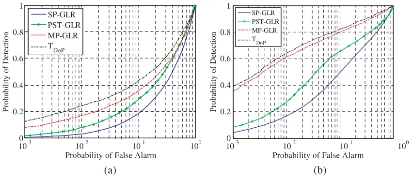
Although the exact ratio of the target to clutter is unknown previously, to compare the detection performance, we ran the DoP, SP-GLR, PST-GLR and MP-GLR detectors against the former datasets. Then we plotted the PD versus PF A curves in Fig. 6, which are also called receiver operating characteristic (ROC). Since the target location in the datasets was a priori knowledge, we divided the detection map into two regions: target and clutter. Then we can calculate the detection probability of the data in the target region by counting the number of pixels in which the statistic is larger than the given threshold asPD. The false alarm probability PF A can be computed from the data in the clutter region by the same way. A pair (PF A, PD) corresponds to a point on the ROC curve.
100-3 10-2 10-1 100 0.2
0.4 0.6 0.8 1
Probability of False Alarm
Probability of Detection
SP-GLR PST-GLR MP-GLR
TDoP
SP-GLR PST-GLR MP-GLR T
DoP
100-3 10-2 10-1 100
0.2 0.4 0.6 0.8 1
Probability of False Alarm
Probability of Detection
(a) (b)
Figure 6. Detector performance for real data collected by IPIX radar on November 18, 1993. (a) Dataset 1. (b) Dataset 2.
6. CONCLUSION
In this paper, we have designed a novel target detector by using statistics of the estimated DoP. We generated the polarimetric radar model at first which includes both target and clutter echoes. Based on the radar model, the PDFs of the estimated DoP for the radar reception were derived from joint eigenvalue distributions of the complex noncentral Wishart matrix. To evaluate the detection performance, we analyzed the probabilities of false alarm and detection. The performance of the new detector was also compared with the SP-GLR, PST-GLR and MP-GLR detectors. At last, we applied the detectors in real collected data. For the proposed detector, the compared results demonstrated an obvious performance improvement with respect to the other typical polarimetric detectors.
REFERENCES
1. Giuli, D., “Polarization diversity in radars,”Proceedings of the IEEE, Vol. 74, No. 2, 245–267, 1986. 2. Novak, L. M., M. B. Sechtin, and M. J. Cardullo, “Studies of target detection algorithms that use polarimetric radar data,”IEEE Transactions on Aerospace and Electronic Systems, Vol. 25, No. 2, 150–165, 1989.
3. Park, H., J. Li, and H. Wang, “Polarization-space-time domain generalized likelihood ratio detection of radar targets,” Signal Processing, Vol. 41, No. 1, 153–164, 1995.
4. Pastina, D., P. Lombardo, and T. Bucciarelli, “Adaptive polarimetric target detection with coherent radar. I. Detection against Gaussian background,”IEEE Transactions on Aerospace and Electronic Systems, Vol. 37, No. 4, 1194–1206, 2001.
5. Hurtado, M. and A. Nehorai, “Polarimetric detection of targets in heavy inhomogeneous clutter,” IEEE Transactions on Signal Processing, Vol. 56, No. 4, 1349–1361, Apr. 2008.
6. Kelly, E. J., “An adaptive detection algorithm,” IEEE Transactions on Aerospaceand Electronic Systems, Vol. 22, No. 1, 115–127, 1986.
7. Born, M. and E. Wolf, Principles of Optics: Electromagnetic Theory of Propagation, Interference and Diffraction of Light, 7th Edition, Cambridge Univ. Press, Cambridge, U.K., 1999.
8. Wolf, E., “Coherence properties of partially polarized electromagnetic radiation,” II Nuovo Cimento, Vol. XIII, No. 6, 1165–1181, Sep. 1959.
10. Galletti, M., D. S. Zrnic, V. Melnikov, and R. J.Doviak, “Degree of polarization at horizontal transmit theory and applications for weather radar,”IEEE Transactions on Geoscience and Remote Sensing, Vol. 50, No. 4, 1291–1301, Apr. 2012.
11. Shirvany, R., M. Chabert, and J. Tourneret, “Estimation of the degree of polarization for hybrid/compact and linear dual-pol SAR intensity images principles and applications,” IEEE Transactions on Geoscience and Remote Sensing, Vol. 51, No. 1, 539–551, Jan. 2013.
12. Shirvany, R., M. Chabert, and J. Tourneret, “Ship and oil-spill detection using the degree of polarization in linear and hybrid/compact dual-pol SAR,” IEEE Journal of Selected Topics in Applied Earth Observations and Remote Sensing, Vol. 5, No. 3, 885–892, Jun. 2012.
13. Del Rio, V. S., J. M. P. Mosquera, M. V. Isasa, and M. E. de Lorenzo, “Statistics of the degree of polarization,” IEEE Transactions on Antennas and Propagation, Vol. 54, No. 7, 2173–2175, Jul. 2006.
14. Medkour, T. and A. T. Walden, “Statistical properties of the estimated degree of polarization,” IEEE Transactions on Signal Processing, Vol. 56, No. 1, 408–414, Jan. 2008.
15. Goodman, N. R., “Statistical analysis based on a certain multivariate complex Gaussian distribution (an introduction),”The Annals of Mathematical Statistics, Vol. 34, 152–177, 1963. 16. James, A. T., “Distributions of matrix variates and latent roots derived from normal samples,”
The Annals of Mathematical Statistics, Vol. 35, No. 1, 475–501, 1964.
17. Gross, K. I. and D. S. P.Richards, “Total positivity, spherical series, and hypergeometric functions of matrix argument,” Journal of Approximation Theory, Vol. 59, 224–246, 1989.
18. Gradshteyn, I. S. and I. M. Ryzhik,Table of Integrals, Series, and Products, 6th Edition, Academic Press, New York, 2000.