Scattering Analysis of Buried Objects by Using FDTD
with Nonuniform Meshes
Min Zhang, Cheng Liao*, Xiang-Zheng Xiong, and Xiaomin Xu
Abstract—This paper presents a finite-difference time-domain (FDTD) method of the infinite half-space with nonuniform meshes, aiming to speed up the FDTD calculation of scattering of buried objects. Two 1-D modified FDTD equations are employed to set plane wave excitation of the infinite half-space scattering problems. In order to reduce calculation time and meshes, a method with nonuniform meshes is applied. Fine grids are used for the buried objects and underground while coarse grids are applied for other regions. The 1-D modified FDTD equations with nonuniform meshes are derived, and the settings of total-field/scattering-field (TF-SF) boundary are given. Finally, the proposed method is applied to calculate the transient scattering field of a buried mine. Numerical results demonstrate the validity of the method, and the simulation time is significantly reduced compared to uniform meshes FDTD.
1. INTRODUCTION
The FDTD method has been successfully used to solve many kinds of scattering problems [1–4], such as the stealth and anti-stealth of aircraft [5, 6] and detecting or imaging of unknown targets [7–9]. It is convenient to implement the FDTD scheme for the scattering of objects in free space. The incident plane wave can be easily set according to the equivalence principle. However, the FDTD TF-SF boundary is much more complex in half-space, especially in layered medium. In order to solve these problems, Wong et al. introduced the three-wave method [10], which needs to calculate the reflection and transmission waves on the interface in advance. It will be more difficult when the infinite half-space becomes layered medium. Winton et al. derived the 1-D modified FDTD equations to simulate plane wave incident to layered media in 2D scheme (TM-wave and TE-wave) [11]. Based on [11], Jiang et al. proposed a Π-shaped TF-SF boundary [12]. By carrying out different operations on each side of the TF-SF boundary, the plane wave can be injected in 3-D problems, even in layered and dispersive medium.
Although the difficulties of injecting the plane wave source for the infinite half-space FDTD has been overcome, many useful techniques of FDTD for free space have not been generalized for half-space geometries. One of them is the nonuniform meshes techniques. It can be found that the methods mentioned before were used in uniform grids. As we know, there are some areas which should frequently apply fine grids in FDTD calculation, such as the complex constructions of targets and underground soil with high dielectric constant. For uniform grids FDTD, coarse meshing leads to low accuracy, and fine meshing costs large amount of computing resources.
In this paper, the 1-D modified FDTD equations based on [11, 12] are derived in a nonuniform meshing scheme. Then the processing of incident plane wave for TF-SF boundary is given. Finally, the scattering fields of a buried mine are calculated, and the simulation time and number of meshes are both significantly reduced compared with uniform meshes FDTD method.
Received 23 November 2016, Accepted 13 January 2017, Scheduled 9 February 2017
* Corresponding author: Cheng Liao ([email protected]).
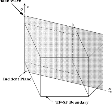
Figure 1. Setting of the TF-SF boundary.
2. THEORY OF THE METHOD
Due to limited memory of computers, the infinite half-space region cannot be directly truncated by absorbing boundary of FDTD method. To overcome the difficulty, a part of the region is selected, and it is surrounded by the absorbing boundary. For a scattering problem in the presence of layered medium, it is difficult to set the TF-SF boundary. The major problem is the prior calculation of incident wave. In order to solve the problem, the 1-D modified FDTD equations are given in [11].
Assume that the TMy and TEy waves propagate in xoz 2-D plane. The incident angle is θ with respect to thez axis, which can be seen in Fig. 1. Then the 1-D modified Maxwell’s equations of TMy wave can be shown as follows.
∂Ey1D
∂z = μ0∂H∂tx1D (1)
1 cos2θ
∂Hx1D
∂z = ε ∂Ey1D
∂t +σEy1D (2)
The equations of TEy wave can be written as: ∂Hy1D
∂z = −ε ∂Ex1D
∂t −σEx1D (3)
1 cos2θ
∂Ex1D
∂z = −μ0∂H∂ty1D (4)
Discretizing Equations (1) and (2) in nonuniform meshes, the 1-D modified FDTD equations with nonuniform scheme can be derived as:
Hn+1/2
x1D (k+ 1/2) =H n−1/2
x1D (k+ 1/2)−
Δt μ(k)Δzk
Eyn1D(k+ 1)−Eyn1D(k)
(5)
En+1 y1D(k) =
2ε(k)−σ(k)Δt
2ε(k)+σ(k)ΔtE n
y1D(k) +
2Δt
2ε(k)+σ(k)Δt
Hn+1/2
x1D (k+ 1/2)−H n+1/2
x1D (k−1/2)
Δhkcos2θ
(6)
where
Δhk = Δzk+Δzk+1
2 (7)
ε(k) = Δzkε(k)+Δzk+1ε(k+ 1) Δzk+Δzk+1
(8)
σ(k) = Δzkσ(k)+Δzk+1σ(k+ 1) Δzk+Δzk+1
Figure 2. 1-D FDTD scheme with non-uniform meshes.
where Δzk is the space step of Ey1D and Δhk the space step ofHx1D, which is shown in Fig. 2. ε(k) is
the weighted mean of ε(k) and ε(k+1), andσ(k) is the weighted mean ofσ(k) and σ(k+1).
The iterative equations of TEy wave can also be derived in the same way. The fields on TF-SF boundary can be given correctly by using the 1-D equations because these equations include the reflection and transmission of the ground.
The setting procedure of TF-SF boundary in 2-D FDTD is as follows: TakingABDC as the TF-SF boundary, which is shown in Fig. 1. First of all, the 1-D modified FDTD is performed once on AB and CD, respectively, where S1 and S2 represent the point sources of the two FDTD calculations. Then the electric fields on AB and CD boundaries can be obtained from the 1-D FDTD results. Because the incident waveform of AC boundary is the same as that of the corner AorC, the incident fields can be derived with a proper time delay of point AorC. The BD boundary may be treated in the same way asAC, which can be extended into the CPML. Assume ΔTAA as the time delay between pointA and A. Then ΔT
AA may be described as in Eq. (10).
ΔTAA=AA·sin (θ)/c0= iA−1
i=iA
Δxi·sin (θ)/c0 (10)
Δxi is the space step in FDTD calculation, which varies with the location of grid. If the time delay is not integral multiple of time step Δt, the linear interpolation will be used. Distinguished from the uniform FDTD, the mesh size of nonuniform FDTD is variable. We can adjust the mesh size to make the most time delays be integral multiple of the time step, then the errors caused by linear interpolation will be reduced.
Taking TMy wave for example, the 1-D modified FDTD results can only provide Ey and Hx components of incident wave. However, Hz component is also needed for the setting of AB and CD boundaries. To obtain the Hz component, a differential calculation is applied. For AB boundary, the 1-D modified FDTD should be performed once on i=iA and i=iA−1, respectively, then theHz on
i=iA−1/2 may be obtained with the following differential equation.
Hn+1/2
z,inc (iA−1/2, k) =Hz,incn−1/2(iA−1/2, k)−u Δt
iA−1ΔxiA−1
En
y1D(iA, k)−Eyn1D(iA−1, k)
(11)
TheHz component oni=iC+ 1/2 should also be obtained in the same way.
The method of injecting incident plane wave source for 2-D FDTD scheme has been introduced as mentioned above. For a 3-D FDTD scheme, a method mentioned in [13] is adopted. Firstly, a major incident plane should be set, shown in Fig. 3. Secondly, perform the 2-D FDTD calculation in the incident plane with the above method. Then project the 3-D TF-SF boundary on the incident plane and calculate the incident source on TF-SF boundary by linear interpolation. Finally, process the 3-D FDTD calculation. It is worth mentioning that the mesh sizes of 2-D FDTD and 3-D FDTD can also be fine-tuned to reduce the errors caused by linear interpolation.
In order to perform the near- to far-field transformation, the equivalence principle can be used in terms of equivalent electric and magnetic currents on a transformation surface that surrounds the scatterer [14].
3. NUMERICAL RESULTS
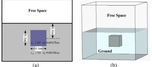
Figure 4 shows a simple buried object that demonstrates the presented method. The dielectric cube has dimensions of 0.1 m×0.1 m×0.1 m, relative permittivity of 2.9, and conductivity of 0.00167 S/m. The center of the cube lies 0.1 m beneath the surface of the ground. The relative permittivity and conductivity of the infinite ground areεr0= 3.0 andσ0= 0.00334 S/m, respectively. The incident plane
wave is Gaussian pulse with pulse width of 2 ns, and the amplitude of electric field is 1.0 V/m. In the simulation, the mesh sizes vary from 15 mm to 25 mm.
Figures 5(a) and (b) show the scattered far field of the buried cube for TM wave incidence with θ = 0◦ and θ = 60◦, respectively. Figs. 6(a) and (b) show the corresponding results for TE wave incidence. It may be seen that all the results are in good agreements with Hill’s results [15].
For TM wave incidence, it can be found that the amplitudes of scattered far fields with θ = 60◦ are bigger than that of θ= 0◦. However for TE wave incidence, the conclusion is on the contrary.
In order to evaluate the errors of the proposed method, the leakages of electric wave in SF region are tested. As the leakages will be merged with the scatter fields, the buried object in Fig. 4 is removed, and
(a) (b)
Figure 4. A dielectric cube buried in infinite ground: (a) section (b) 3D view.
Table 1. The leakages of non-uniform meshes FDTD and uniform meshes FDTD.
Name Non-uniform FDTD Uniform FDTD
θ= 0◦ θ= 60◦ θ= 0◦ θ= 60◦ Leakages for TM incidence (V/m) 5.436E-4 2.436E-3 3.756E-4 1.561E-3
90 120 150 180 210 240 270 0.0 1.0x10⁻⁴ 2.0x10⁻⁴ 3.0x10⁻⁴ 4.0x10⁻⁴ 5.0x10⁻⁴ (r / λ ) | Es /E0 |
θ Degree
Hill’s Result NHF-FDTD
90 120 150 180 210 240 270 0.0 1.0x10⁻⁴ 2.0x10⁻⁴ 3.0x10⁻⁴ 4.0x10⁻⁴ 5.0x10⁻⁴ 6.0x10⁻⁴ 7.0x10⁻⁴ 8.0x10⁻⁴ (r / λ ) | Es /E0 |
θ Degree
Hill’s Result NHF-FDTD
(a) (b)
Figure 5. Scattered far fields for TM wave incidence at 0.6 GHz: (a) incident angleθ= 0◦, (b) incident angle θ= 60◦.
(a) (b)
90 120 150 180 210 240 270 0.0 1.0x10⁻⁴ 2.0x10⁻⁴ 3.0x10⁻⁴ 4.0x10⁻⁴ 5.0x10⁻⁴ (r / λ ) | Es /E0 |
θ Degree
Hill’s Result NHF-FDTD
90 120 150 180 210 240 270 0.0 1.0x10⁻⁴ 2.0x10⁻⁴ 3.0x10⁻⁴ 4.0x10⁻⁴ (r / λ ) | Es /E0 |
θ Degree
Hill’s Result NHF-FDTD
Figure 6. Scattered far fields for TE wave incidence at 0.6 GHz: (a) incident angleθ= 0◦, (b) incident angle θ= 60◦.
Mine Wavefront
First Layer
Second Layer 1
r 1= 4. 5
2
r 2= 8. 0 = 3mS/m
Mine 0. 3m 0.25m 0.225m Probe B Probe A 0. 3m Wavefront
ε σ=3 mS/m
ε σ
(a) (b)
0 2 4 6 8 10 12 14 16 -0.6
-0.4 -0.2 0.0 0.2 0.4 0.6 0.8 1.0
E
y (V
/m
)
t (ns)
uniform mesh non-uniform mesh
0 2 4 6 8 10 12 14 16 -0.2
-0.1 0.0 0.1 0.2 0.3 0.4 0.5 0.6
E
y (V
/m
)
t (ns)
uniform mesh non-uniform mesh
(a) (b)
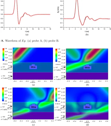
Figure 8. Waveform ofEy: (a) probe A, (b) probe B.
(b)
(d) (a)
(c)
Figure 9. Electric fields of different time inxoz plane: (a) t= 2.0 ns, (b) t= 4.0 ns, (c) t= 5.5 ns, (d) t= 7.0 ns.
a plane wave injected to ground is simulated. Uniform meshes FDTD is also used for the simulation, and the mesh size is 15 mm. Table 1 shows the maximum leakages of electric wave for different incidences. Leakage of oblique incidence is lager than that of normal incidence. TM wave incidence produces more leakages than TE wave. The nonuniform differential scheme may increase errors, and it leads to more leakages than uniform meshes.
Table 2. The mesh size and time needed by the two methods for the simulation of buried mine.
Name Smallest Mesh Largest Mesh Meshes Run Time
Non-uniform 10 mm 22 mm 0.408 million 47.2 sec
Uniform 10 mm 10 mm 1.152 million 128.9 sec
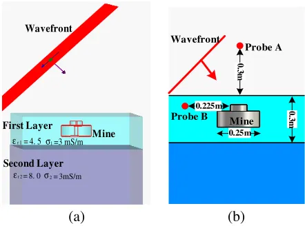
A= 1 V/m. It can be seen in Fig. 7 that the infinite ground has two layers withεr1 = 4.5σ1 = 3 mS/m
andεr2 = 8.0σ2= 3 mS/m for top and bottom, respectively. The dimensions of the mine are: diameter
R= 0.25 m and thicknesst= 0.1 m.
The waveforms of electric fieldEy in positions A and B are shown in Figs. 8(a) and (b), respectively. The results obtained from the proposed method are in good agreements with that of the uniform mesh FDTD. The size of meshes, number of meshes and time cost are shown in Table 2. In uniform FDTD simulation, the mesh sizes are 10 mm. But in nonuniform FDTD simulation, the mesh sizes vary from 10 mm to 22 mm. It costs only 47.2 seconds by using proposed method, meanwhile 128.7 seconds is needed for uniform mesh FDTD.
Figures 9(a), (b), (c) and (d) show the electric fields of different times inxoz plane, respectively. The reflected wave can be seen when plane wave reaches the interfaces. There are also obviously scattered fields around the mine.
4. CONCLUSIONS
This paper presents a novel method for fast calculation of the scattering fields of buried objects. By utilizing nonuniform mesh in a 1-D modified FDTD, the plane wave is injected successfully, and the computing resources can be saved significantly. A dielectric cube buried in infinite media is used to validate this method. The scattered far fields predicted by the method are in good agreements with Hill’s. Moreover, the method is applied to the scattering calculation of a mine buried in layered medium, and significant reductions of calculation time and meshes are obtained.
ACKNOWLEDGMENT
This work was supported by the National Basic Research Program of China (973 Program, Grant No. 2013CB328904) and the Joint Fund of the National Natural Science Foundation of China and the China Academy of Engineering Physics (NSAF, Grant No. U1330109).
REFERENCES
1. Zainud-Deen, S. H., A. Z. Botros, and M. S. Ibrahim, “Scattering from bodies coated with metamaterial using FDTD method,” Progress In Electromagnetics Research B, Vol. 2, 279–290, 2008.
2. Hu, X.-J. and D.-B. Ge, “Study on conformal FDTD for electromagnetic scattering by targets with thin coating,” Progress In Electromagnetics Research, Vol. 79, 305–319, 2008.
3. Wang, M. Y., J. Xu, J. Wu, et al., “FDTD study on scattering of metallic column covered by double-negative metamaterial,”Journal of Electromagnetic Waves and Applications, Vol. 21, No. 14, 1905– 1914, 2007.
4. Yang, L.-X., D.-B. Ge, and B. Wei, “FDTD/TDPO hybrid approach for analysis of EM scattering of combinative objects,” Progress In Electromagnetics Research, Vol. 76, 275–284, 2007.
5. Holland, R., “Two-pass finite-difference time-domain (FDTD) calculations on a fighter aircraft,” IEEE Trans. Antennas Propag., Vol. 44, No. 5, 659–664, 1996.
7. Liu, Y. and L. X. Guo, “FDTD investigation on GPR detecting of underground subsurface layers and buried objects,”2016 IEEE MTT-S International Conference on NEMO, 1–2, 2016.
8. Fhager, A., S. K. Padhi, and J. Howard, “3D image reconstruction in microwave tomography using an efficient FDTD model,”IEEE Antennas Wireless Propag. Lett., Vol. 8, 1353–1356, 2009. 9. Ozt¨¨ urk, E., E. Ba¸saran, and S. Aksoy, “Numerical modeling of ground penetrating radar,”
SubChapter in Subsurface Sensing Book, from J. Wiley & Sons Inc., 2011.
10. Wong, P., G. Tyler, J. Baron, E. Gurrola, and R. Simpson, “A three-wave FDTD approach to surface scattering with applications to remote sensing of geophysical surfaces,” IEEE Trans. Antennas Propag., Vol. 44, No. 4, 504–513, 1996.
11. Winton, S. C., P. Kosmas, and C. M. Rappaport, “FDTD simulation of TE and TM plane waves at nonzero incidence in arbitrary layered media,” IEEE Trans. Antennas Propag., Vol. 53, No. 5, 1721–1728, 2005.
12. Jiang, Y. N., D. B. Ge, and S. J. Ding, “Analysis of TF-SF boundary for 2D-FDTD with plane P-wave propagation in layered dispersive and lossy media,”Progress In Electromagnetics Research, Vol. 83, 157–172, 2008.
13. Capoglu, I. R. and G. S. Smith, “A total-field/scattered-field plane-wave source for the FDTD analysis of layered media,” IEEE Trans. Antennas Propag., Vol. 56, No. 1, 158–169, 2008.
14. Demarest, K., Z. Huang, and R. Plumb, “An FDTD near- to far-zone transformation for scatterers buried in stratified grounds,”IEEE Trans. Antennas Propag., Vol. 44, No. 8, 1150–1157, 1996. 15. Hill, D. A., “Electromagnetic scattering by buried objects of low contrast,” IEEE Trans. Geosci.